Hierarchical Federated Learning for Edge-Aided Unmanned Aerial Vehicle Networks

Abstract

Federated learning (FL) allows UAVs to collaboratively train a globally shared machine learning model while locally preserving their private data. Recently, the FL in edge-aided unmanned aerial vehicle (UAV) networks has drawn an upsurge of research interest due to a bursting increase in heterogeneous data acquired by UAVs and the need to build the global model with privacy; however, a critical issue is how to deal with the non-independent and identically distributed (non-i.i.d.) nature of heterogeneous data while ensuring the convergence of learning. To effectively address this challenging issue, this paper proposes a novel and high-performing FL scheme, namely, the hierarchical FL algorithm, for the edge-aided UAV network, which exploits the edge servers located in base stations as intermediate aggregators with employing commonly shared data. Experiment results demonstrate that the proposed hierarchical FL algorithm outperforms several baseline FL algorithms and exhibits better convergence behavior.

1. Introduction

1.1. Motivations

Owing to the recent advances in the Internet of Things (IoT), there has been a bursting increase in heterogeneous and private data generated from various sensors, mobile phones, smart home appliances and unmanned aerial vehicles (UAVs) [1]. Particularly, UAVs are proving to be one of the key enablers in gathering data from applications, such as road extraction [2], traffic management [3] and remote sensing, due to their mobility and cost effectiveness [4]. Naturally, therefore, there is a huge demand to construct machine learning models for such data while keeping the privacy.

Federated learning (FL) is an efficient and promising solution to realize such a goal [5], and its applications in unmanned aerial vehicle (UAV) networks have attracted significant attention in both industrial and academic sectors [4]. With the aid of FL, a global machine learning model can be efficiently trained without the need for each UAV to directly send its private data to a cloud (or edge) server. This can be realized through the following four cyclic steps: (i) training a global model locally at each UAV (i.e., local model) with its own data, (ii) reporting the trained local models of the UAVs to a centralized cloud server, (iii) aggregating the local models at the cloud server to update the global model, and (iv) sending the updated global model to the UAVs for training it at the UAVs locally again. Most of the FL systems use the FedAvg algorithm, which averages the model updates weighted by the number of samples that they are trained on. Although the FL (without the need to send the real-time data feed to the cloud server) can reduce the latency and bandwidth, the ever-growing size of deep learning (DL) models causes the transmission of model updates to be a bottleneck of the system [6]. Additionally, in practice, a very critical issue for the FL in the edge-aided UAV network is how to handle the non-independent and identically distributed (non-i.i.d.) nature of heterogeneous data acquired by various types of UAVs while ensuring the convergence of training the global model [7].

1.2. Related Works

Intermediate edge servers that are located in base stations between UAVs and a cloud server (usually, more close to the UAVs) can help significantly reduce both communication and computation costs required by the FL [8,9,10]. Zhang et al. [11] considered a FL system with a ground fusion center (GFC) acting as an aggregator to deploy the UAV network in remote locations in order to reduce the communication complexity. On the other hand, the authors of [12] used the UAVs as a communication link between the users and edge notes to mitigate the network latency overhead. Zhang et al. [13] proposed using multi-dimensional contracts to create an incentive mechanism between the UAVs and task publishers, which can increase the number of UAV providers that collaborate with the FL system owners. The authors [14] formulated several services: computational offloading, resource allocation, and optimal UAV location in a mobile edge computing network, while using the UAVs as both a communication and computational device. Almost all of the above works involve UAVs as an active part of the network system, but they do not take data heterogeneity of the generated samples into account. Another important consideration in UAV networks is that the UAVs are practically constrained by the memory, communication, computation, and energy consumption. This leads to a low participation rate of the UAVs, which will eventually affect the performance of the model [15]. Proposed methods that solve the system heterogeneity issues include using distributed learning to perform the training process across multiple edge devices [16,17], choosing the proficient devices by predicting outages and resource information of the critical infrastructure agents [18]. Even though most of the above-mentioned studies use FL as a base model, they do not consider extreme non-i.i.d. situations that arise when the deployment structures and generated data distributions of the UAV networks among different edge servers differ significantly. Several studies [19,20,21] have investigated the performance issue of the FL in non-i.i.d environments, but in the absence of edge servers. Unfortunately, therefore, the results of these works are not applicable to developing an effective FL algorithm in the edge-aided UAV network. The authors of [22,23] developed several effective FL algorithms for edge-aided networks. However, when the number of edge servers is large, which is the most realistic situation in the edge-aided UAV network, the performance of such algorithms is relatively low (and thus, might be unsatisfactory in practice) due to the wide divergence of data available at the edge servers [24]. In addition, some researchers have tried to include the edge servers in the training process for UAV networks [13,25,26,27,28], but the edge servers still do not actively participate in the aggregation process.

To the best of our knowledge, in the literature, the aforementioned limitations have not been broken through yet, and developing high-performing FL algorithms for the edge-aided UAV network that is robust in non-i.i.d. data distributions is still an active area of research.

1.3. Contributions

The main contributions of our work are two-fold as follows:

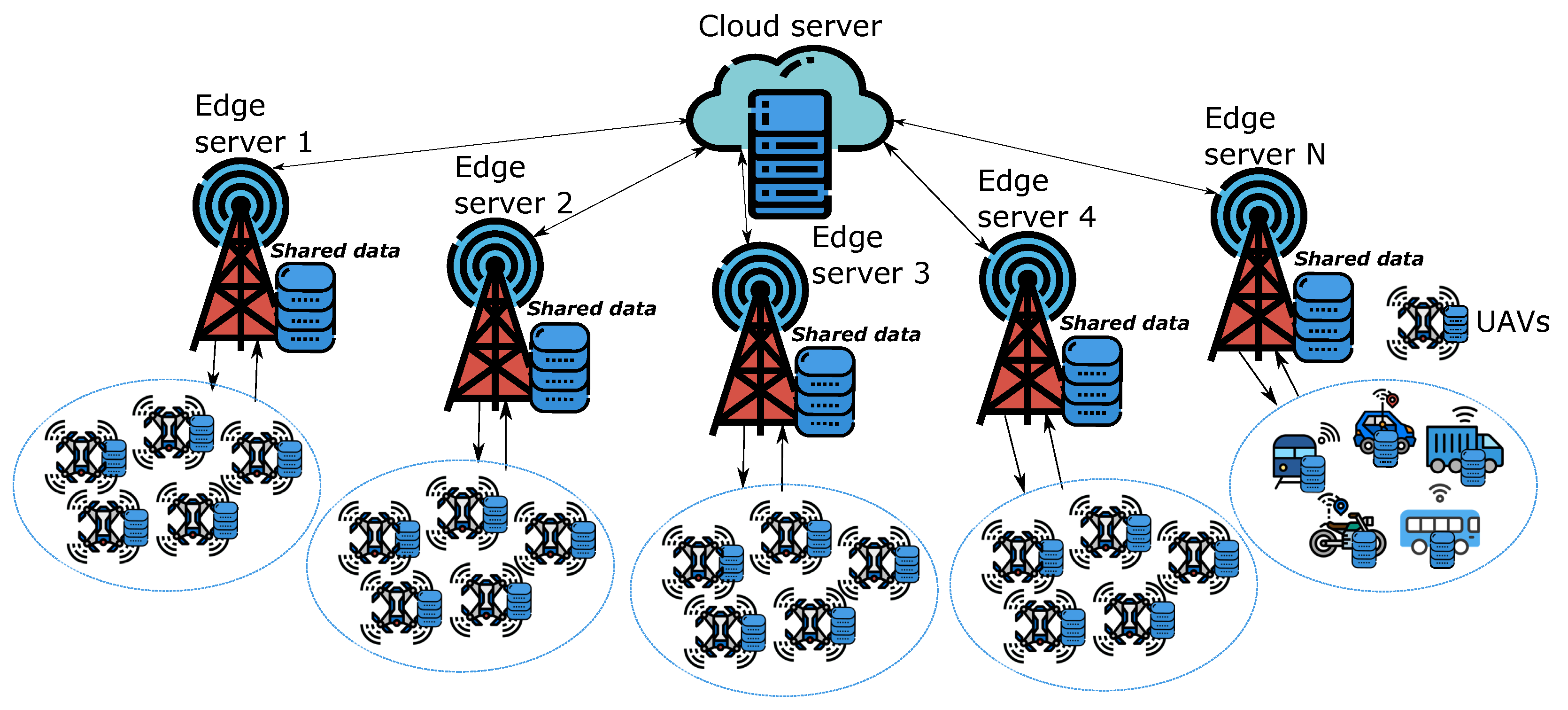
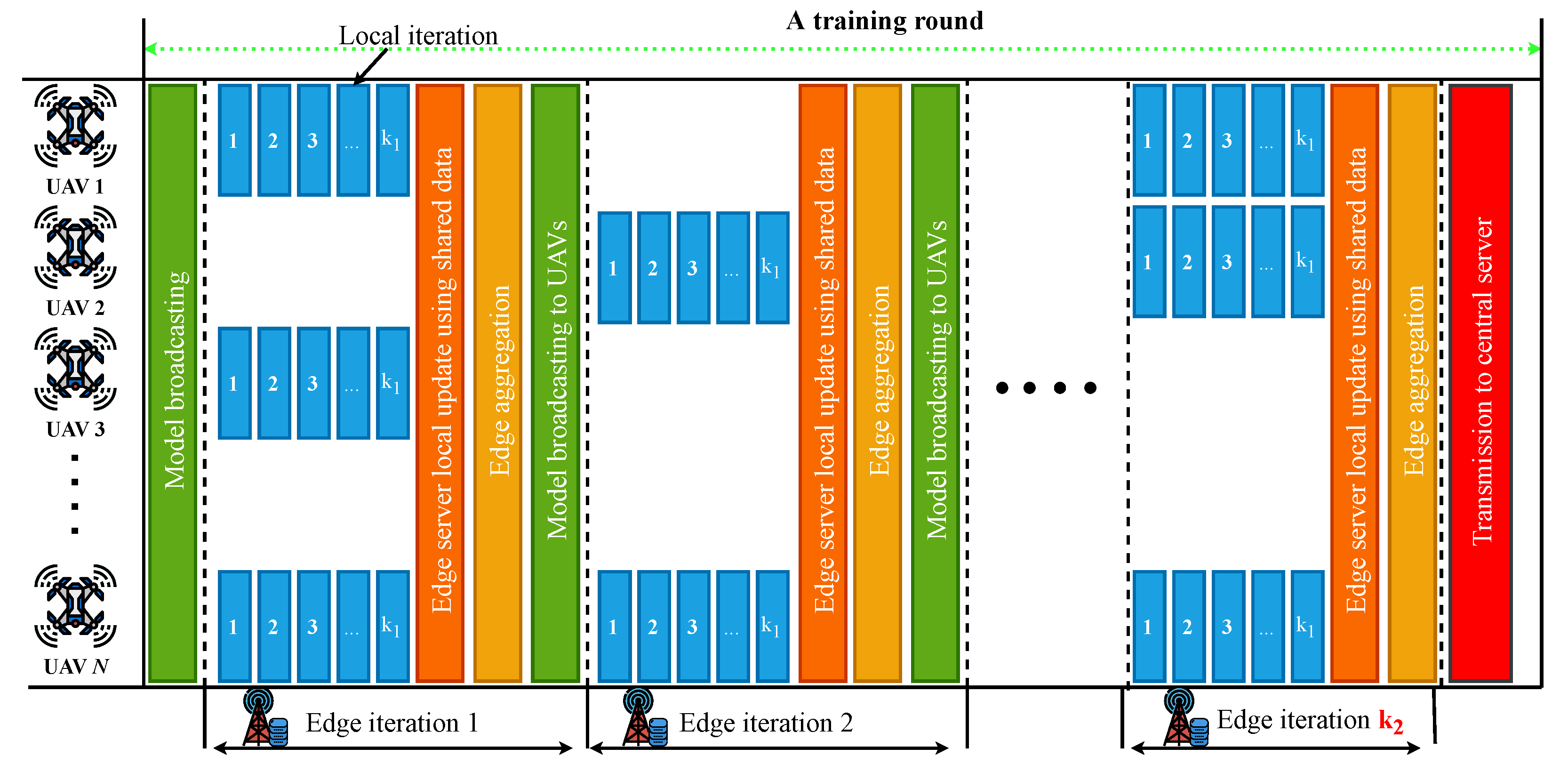
• We develop a novel and high-performing FL scheme, namely, the hierarchical FL algorithm, for the edge-aided UAV network that works well in real-world scenarios with non-i.i.d data distributions (i.e., highly skewed feature and label distributions). In this algorithm, we make an innovative idea to employ commonly shared data at the edge servers to effectively solve the divergence issue caused by the non-i.i.d. nature. In practice, this idea is realizable since the commonly shared data can be made or constructed on the edge servers offline by collecting exemplary data samples from the UAVs. We also present an effective method to hierarchically aggregate the local models of both the UAVs and the edge servers for the global model update.
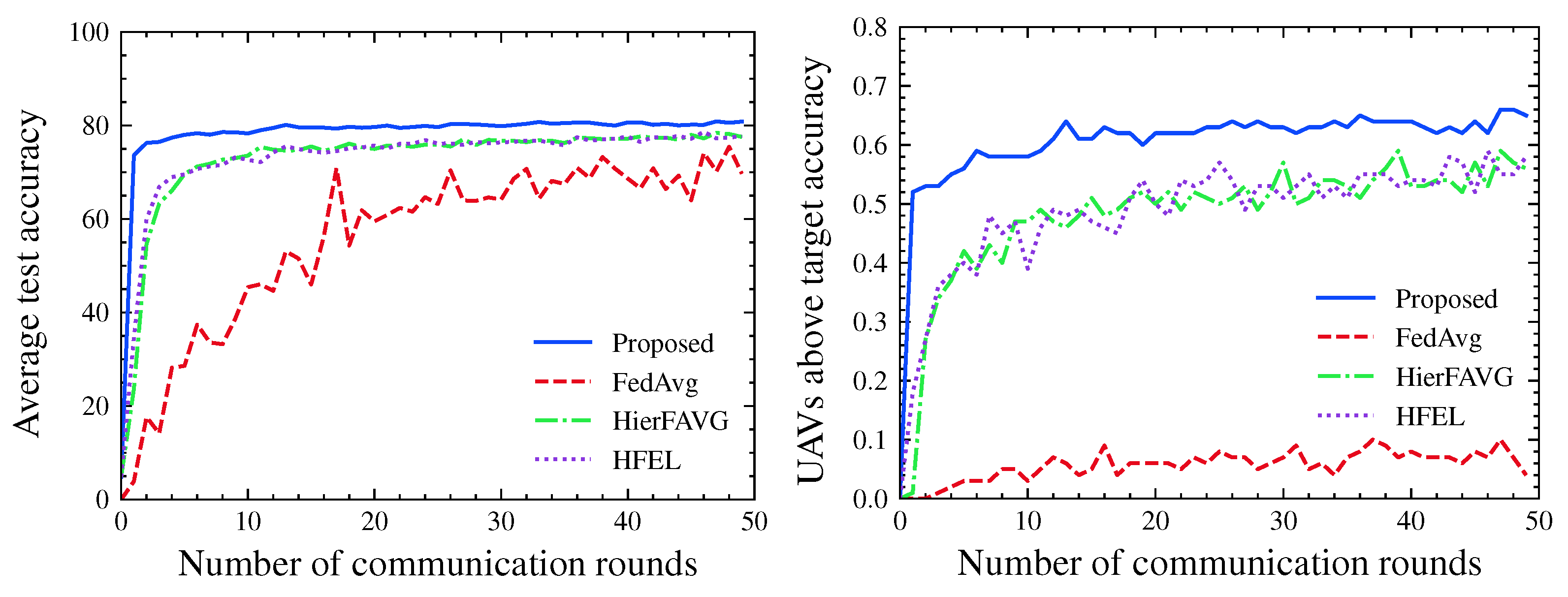
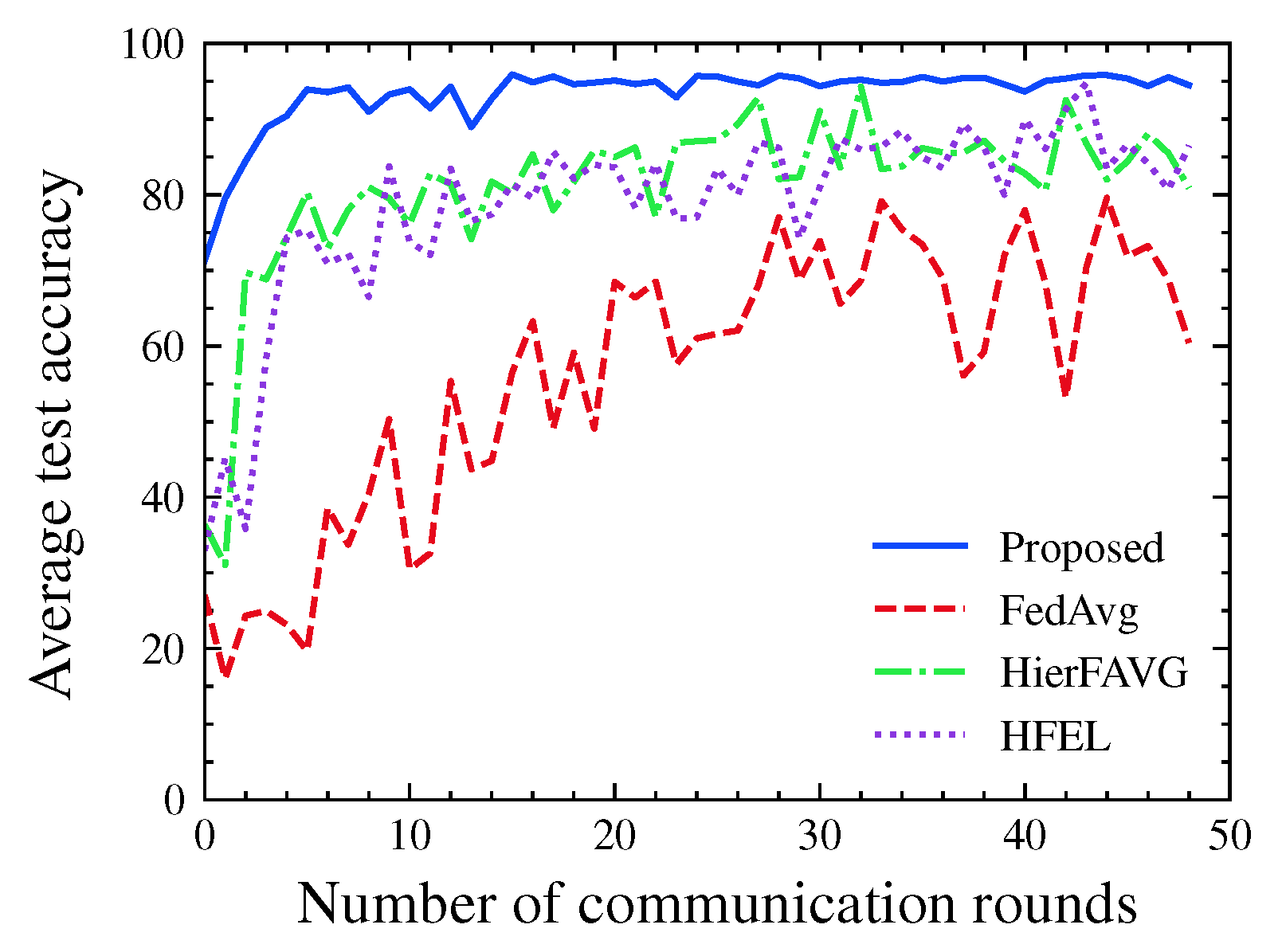
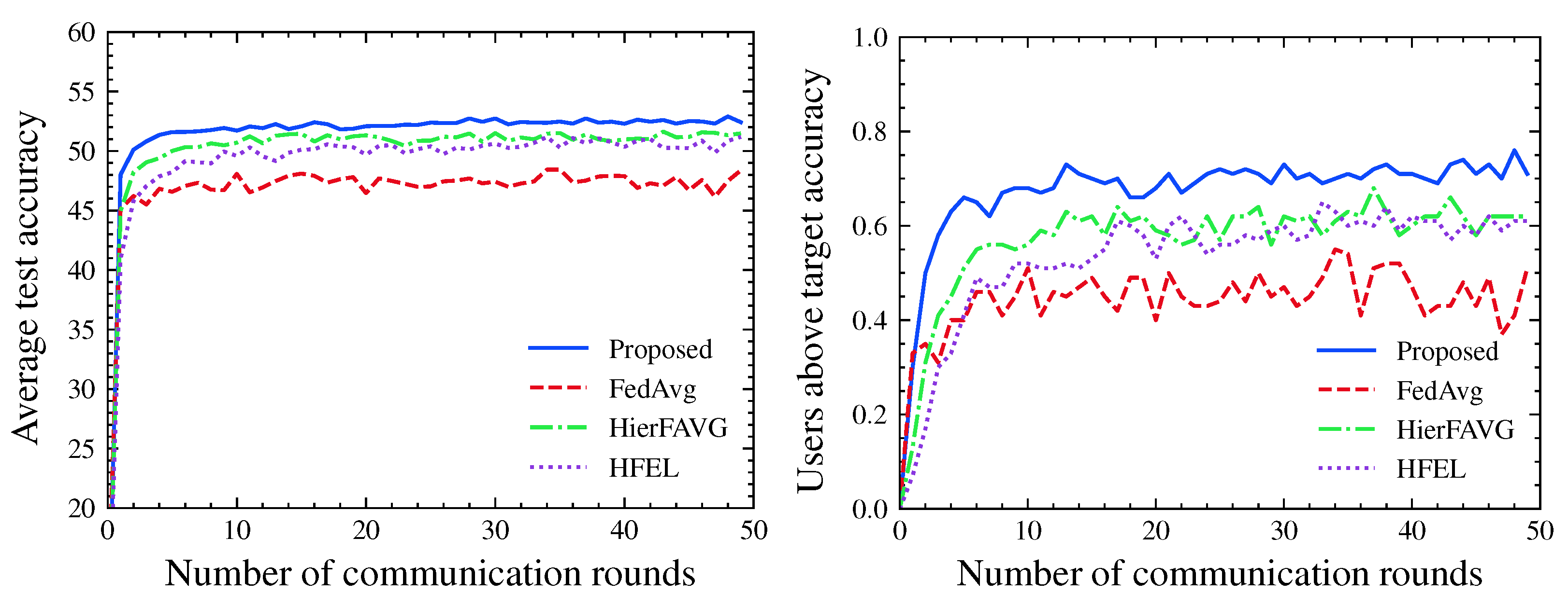
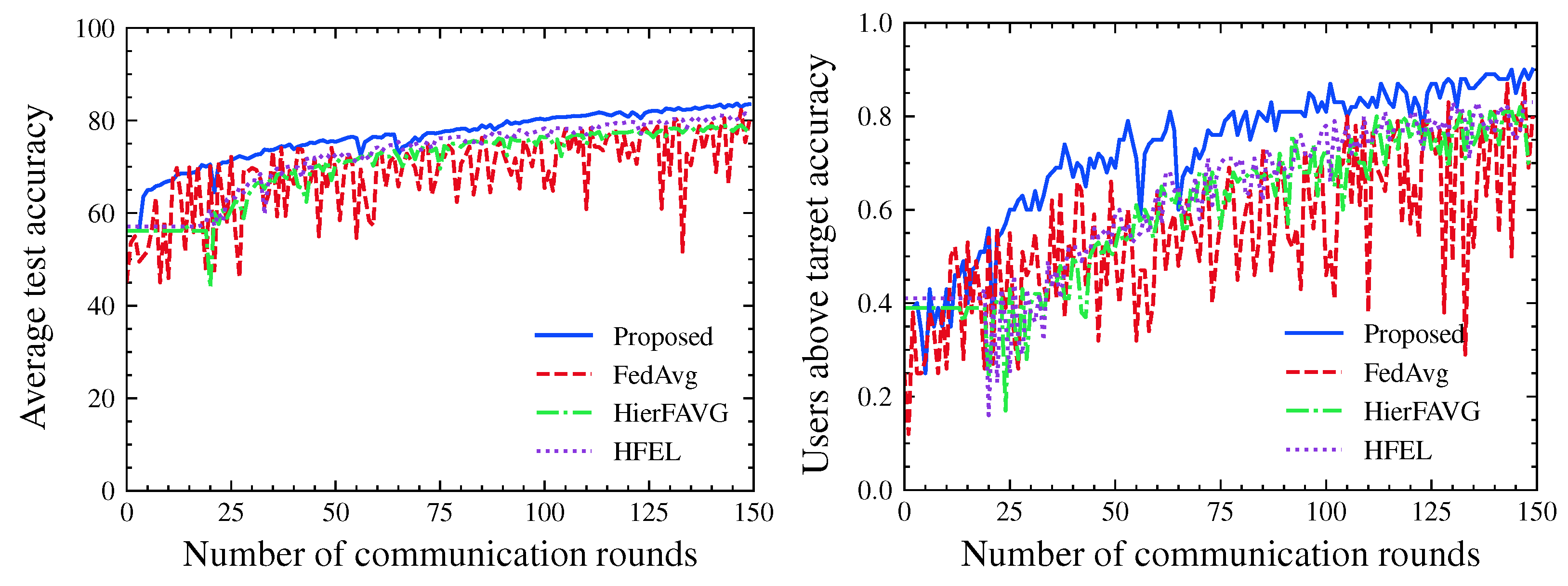
• We present extensive numerical results under various degrees of non-i.i.d data distributions, especially including several extreme situations with label distribution skew in order to demonstrate the superiority and effectiveness of the proposed hierarchical FL algorithm, compared to other baseline FL algorithms. From the numerical results, we also provide useful and insightful guidelines on how the hyperparameters of the hierarchical FL can be set and used in practical UAV networks with edge servers.

2. System Model and Problem Description

As shown in Figure 1, we consider an edge-aided UAV network that includes one cloud server, L edge servers located in base stations, and N UAVs. The UAVs are divided into L groups, and the lth group of UAVs, denoted by ${\mathcal{𝒞}}_l$ with cardinality $|{\mathcal{𝒞}}_l|=C_l$, is assigned to the lth edge server.

Let n be the total number of data samples across the UAVs, where the ith UAV has a dataset, denoted as ${\mathcal{𝒫}}_i$, consisting of $n_i$ data samples. The objective of the FL is to minimize the following (global) loss function:

$$f\left(w\right)=\sum _{i=1}^N\frac{n_i}{n}{F}_i\left(w\right)\mathrm{where}{F}_i\left(w\right)=\frac{1}{n_i}\sum _{j\in {\mathcal{𝒫}}_i}{f}_j\left(w\right).$$

(1)

In Equation (1), $f\left(w\right)$ denotes the loss function for the global model w, and $f_j\left(w\right)$ is the loss function for the jth data sample of the ith UAV.

In the naive FL, the training process begins with the central cloud server sending the global model w to the UAVs [5]. Then, at each step t, the ith UAV trains the global model w locally, which results in a local model $w_i$, using its private dataset ${\mathcal{𝒫}}_i$ based on the gradient descent method as

$$w_i(t+1)=w_i\left(t\right)-{\eta }_t\nabla F_i\left(w\left(t\right)\right)$$

(2)

where ${\eta }_t$ denotes a step size. After sending the local models $\left\{w_i\right\}$ back to the central cloud server, the global model w is updated via the following aggregation: $w(t+1)\leftarrow {\sum }_{i=1}^N\frac{n_i}{n}{w}_i\left(t\right)$. The above procedure is repeated until a desired accuracy is achieved.

Suppose that the global model is updated in every k steps; otherwise, the local models are trained. Then it follows that

$${\mathbf{w}}_i(t+1)=\left\{\begin{array}{cc}{w}_i\left(t\right)-{\eta }_t\nabla F_i\left(w_i\left(t\right)\right),\hfill & \mathrm{if}rem(t,k)\ne 0\hfill \\ \sum _{i=1}^N\frac{n_i}{n}{w}_i\left(t\right)\hfill & \mathrm{if}rem(t,k)=0\hfill \end{array}\right.$$

(3)

where $rem(a,b)$ denotes the remainder when a is divided by b.

Non-Identical Distributions among UAVs

Given the differences in commercial types of UAVs and their hardware, the data acquired by those different UAVs are highly likely to be non-i.i.d. This is especially the case of the FL in the practical UAV networks, compared to the traditional machine learning, where the training data are expected to be uniform. Therefore, heterogeneity of the UAVs leads to poor performance and convergence behavior of the FL due to the large deviation among the local models trained at the devices [20]. Under these circumstances, training a model $F_k$ in its data $P_k$ will not be representative of the joint global model f [19]:

$${\mathbb{E}}_{P_k}\left[F_k\left(w\right)\right]\ne f\left(w\right)$$

(4)

There are several ways in which the data among devices can be deviated from being i.i.d:

• Feature distribution skew: The marginal distributions ${\mathcal{𝒫}}_i$ vary among the devices. That means the features of data are different between the devices. For example, the picture of the same object might differ in terms of brightness, occlusion, camera sensor, etc.
• Label distribution skew: The marginal distributions ${\mathcal{𝒫}}_i$ variance, where devices have access to a small subset of all available labels. For example, each device has access to a couple of images of a certain digit.
• Concept shift (different features, same label): The conditional distributions ${\mathcal{𝒫}}_i\left(x\right|y)$ vary among the devices. This is the case where the same label y might have different features x among devices. In the digit recognition case, digits might be written in drastically different ways, which results in varying underlying features for the same digit.
• Concept shift (same features, different label): The conditional distributions ${\mathcal{𝒫}}_i\left(x\right|y)$ vary among the devices. Here, similar features might be labeled differently across devices. For example, different digits are written in very similar ways, such as 5 and 6, or 3 and 8.

In real-world scenarios, at least each of the above ways can occur in practice, and most datasets usually contain a mixture of them. The problem becomes even more severe in the edge-aided UAV network due to the existence of additional intermediate nodes (i.e., edge servers).

3. Hierarchical FL Algorithm

The key idea of the proposed hierarchical FL algorithm is that the edge servers are used as intermediate aggregators with commonly shared data to improve the performance of learning, even with non-i.i.d data. For this purpose, in practice, one can collect exemplary data samples from the UAVs and employ them as the commonly shared data.

In the hierarchical FL, the commonly shared data are used to train the local models at the edge servers. In addition, we suggest aggregating the local models of both the UAVs and edge servers hierarchically. Detailed explanations are given in the following.

The proposed hierarchical FL algorithm for the edge-aided UAV network is presented in Algorithm 1, where T is the overall aggregation step. In addition, C denotes the fraction of UAVs participating in the hierarchical FL, which are selected from the total N UAVs.

Algorithm 1 works as follows: First, the local models of the UAVs and the edge servers are all initialized with random weights $w_0$, and each edge server is assigned the commonly shared public dataset $\mathcal{𝒬}$ that is equivalent to 5% of the overall dataset. Then, the UAVs and edge servers start training their local models (i.e., the global model of the previous round) in parallel using their private and commonly shared data, respectively. In every step of the global aggregation, the UAVs update their models with globally aggregated parameters $w_t$ from the previous round. By averaging the model update, the magnitude of poisoned models can be reduced in the case of attack, which ensures that the single backdoor has less effect on the overall update procedure.

Algorithm 1 Proposed hierarchical FL algorithm.

1: Initialize $w_0$ and $\mathcal{𝒬}$ 2: for$t=0,1,\cdots T-1$do 3:     for each edge $l=1,\cdots ,L$ do // in parallel 4:         ${\left\{w_i^l\right\}}_{i\in {\mathcal{𝒞}}_l}\leftarrow w_t$ 5:         for $k=1,2,\cdots k_2$ do 6:            for each UAV $i\in {\mathcal{𝒞}}_l$ do // in parallel 7:                for $j=1,2,\cdots k_1$ do 8:                    $w_i^l\leftarrow$ LocalUpdate($i,w_i^l,{\mathcal{𝒫}}_i$) in Algorithm 2 9:                end for 10:           end for 11:           $w^l\leftarrow$ EdgeAggregation(l, ${\left\{w_i^l\right\}}_{i\in {\mathcal{𝒞}}_l}$) in Algorithm 3 12:        end for 13:    end for 14:    $w_{t+1}\leftarrow$ GlobalAggregation(${\{w}_t^l{\}}_{l=1}^L)$ in Algorithm 4 15: end for

Algorithm 2 Local update procedure.

1: functionLocalUpdate($w,\mathcal{𝒫}$) 2:     $\mathcal{ℬ}\leftarrow$ (split $\mathcal{𝒫}$ into batches of size B) 3:     for each local epoch i from 1 to $k_1$ do 4:         for batch $b\in \mathcal{ℬ}$ do 5:            $w\leftarrow w-\eta \nabla (w;b)$ 6:         end for 7:     end for 8:     return w 9: end function

After $k_1$ local iterations, each UAV sends its local model $w_i^l$ trained with private dataset ${\mathcal{𝒫}}_i$ to the edge servers. Upon receiving the local models from the corresponding UAVs, the edge servers perform the EdgeAggregation procedure in Algorithm 3, wherein the local models $w_l^e$ of the edge servers are trained with the shared dataset $\mathcal{𝒬}$ and those are then aggregated together with the local models of the UAVs.

Algorithm 3 Edge aggregation procedure.

1: functionEdgeAggregation($l,{\left\{{\mathbf{w}}_i^l\right\}}_{i\in {\mathcal{𝒞}}_l}$) 2:     $w^l\leftarrow {\sum }_{i=1}^{C_l}\frac{n_l^i}{n_l}{w}_i^l$ 3:     $w_e^l\leftarrow$ LocalUpdate($w^l,\mathcal{Q}$)) // Edge local update 4:     return $\frac{w^l+w_e^l}{2}$ 5: end function

After $k_2$ iterations of the EdgeAggregation procedure, the edge servers send their aggregated models ${\left\{w_t^l\right\}}_{l=1}^L$ to the cloud server, where the global model $w_{t+1}$ is obtained according to the GlobalAggregation procedure in Algorithm 4. Overall, the local update at the ith UAV assigned to the lth edge server takes the following form:

$${\mathit{w}}_i^l(t+1)=\left\{\begin{array}{cc}{w}_i^l\left(t\right)-{\eta }_t\nabla F_i^l(w_i^l\left(t\right),{\mathcal{𝒫}}_i),\hfill & rem(t,k_1)\ne 0\hfill \\ \begin{array}{c}\hfill \frac{1}{2}\left[\sum _{i\in {\mathcal{𝒞}}_l}\frac{n_i}{n_l}{w}_i^l\left(t\right)+w^l\left(t\right)\right]\end{array}\hfill & \begin{array}{c}\hfill rem(t,k_1)=0\\ \hfill rem(t,k_2)\ne 0\end{array}\hfill \\ \sum _{l=1}^L\frac{n_l}{n}{w}^l\left(t\right),\hfill & \hfill rem(t,k_1{k}_2)=0\end{array}\right.,$$

(5)

which is clearly different from that of the traditional FL in Equation (3). We note that when the intermediate aggregator is unable to perform the EdgeAggregation procedure due to the low system resources, which is the case when $k_1=1$ and $w^l\left(t\right)={\sum }_{i\in {\mathcal{𝒞}}_l}\frac{n_i}{n_l}{w}_i^l\left(t\right)$, the overall process reduces to FedAvg Equation (3).

Algorithm 4 Global aggregation procedure.

1: functionGlobalAggregation(${\left\{{\mathbf{w}}_t^l\right\}}_{l=1}^L$) 2:     $w_{t+1}\leftarrow {\sum }_{l=1}^L\frac{n_l}{n}{w}_t^l$ 3:     return $w_{t+1}$ 4: end function

In any FL algorithm, there is a decrease in the accuracy of training a machine learning model compared to the centralized learning method due to the weight divergence, which is mainly caused by the following two factors: different initialization of the models of the UAVs in the training process and the non-i.i.d nature of the underlying data distribution [20]. As a result, there are two important factors that should influence the performance of the proposed hierarchical FL algorithm. The first one is the number $k_1$ of iterations in the local updates of the UAVs and the number $k_2$ of aggregation steps in the edge server before transmitting the update result to the global server.

Lower values of $k_1$ and $k_2$, that is, fewer iterations steps between global aggregations, will reduce the communication cost in practice.

The percentage of commonly shared data $\mathcal{𝒬}$ is the second factor.

Since the edge servers act as aggregators in the hierarchical FL, it is possible for the edge servers to fine-tune the sizes of the shared dataset independently depending on the data distributions of the UAVs assigned to them. The overall training process is shown in Figure 2.

Complexity Analysis

Suppose the completion time for the UAV to finish a single training round is $t_u$, the transmission time of the UAV updates to the edge server is $t_e$, the transmission time of aggregated model updates from the edge servers to central server is $t_c$, and the overall communication time complexity in each round is $\mathcal{𝒪}(CN{t}_e+L{t}_c)$. Since the edge server also acts as a base station between UAVs and central server, the communication time complexity of FedAvg is $\mathcal{𝒪}\left(CN(t_e+t_c)\right)$. Since the active number of users $CN$ is magnitudes higher than the number of edge servers L, our proposed algorithm yields a small communication complexity compared to FedAvg.

4. Numerical Results

In simulations, we consider the image classification task to evaluate and compare the performance of the various FL algorithms. In this task, we consider two scenarios with different degrees of non-i.i.d. data distributions.

First, in Scenario I, the widely used MNIST dataset [29] is set to the private dataset ${\mathcal{𝒫}}_i$ at the UAVs as well as the commonly shared dataset $\mathcal{𝒬}$ at the edge servers. To consider the situation with extremely non-i.i.d. data distribution, 100 UAVs and 10 edge servers are selected such that each UAV is given the data samples only with one class and each edge server is assigned 10 UAVs with 2 different classes in total (for example, the first edge server can be assigned the labels 3 and 5, and thus, each UAV assigned to it has the data samples only with either the label 3 or 5). This scenario well describes the case with label distribution skew, i.e., both when each UAV has the data samples only with one class and when each edge server is assigned the UAVs that have the same labels.

Second, in Scenario II, the Federated Extended MNIST (FEMNIST) dataset [30] is used to classify 52 handwritten uppercase and lowercase letters in addition to the 10 digits, and the dataset is divided according to the writer of the characters with an unbalanced number of samples per UAV. The purpose of considering this scenario is to study the impact of feature distribution skew on the FL, where ${\mathcal{𝒫}}_i$ is set to be different among the UAVs.

In total, 360 UAVs are assigned to 18 edge servers randomly. In both Scenarios I and II, 5% of the dataset is selected as a shared dataset for the edge servers. The dynamical nature of the UAV networks can lead to some of the devices being the bottleneck in the system (i.e., the straggler effect).

Finally, in Scenario III, we also perform experiments using a very low value of $C=0.008$, to demonstrate the robustness of our system to high dropout or low participation rates due to the straggler effects. We use similar settings to Scenario II, while increasing the number of users from FEMNIST dataset to 3500.

In addition, for the purpose of performance comparison, we report the accuracy of the model in every $k_1{k}_2$ times.

For the MNIST dataset in Scenario I, we construct a convolutional neural network (CNN) with four layers: the first two convolutional layers using 10 and 20 filters, respectively, with a kernel size of 5, followed by two fully connected layers with 50 and 10 units, respectively. The FEMNIST dataset in Scenario II is evaluated using a similar CNN: two convolutional layers using 32 and 64 filters with a kernel size of 5 and two fully connected layers with 1024 and 62 units. At each UAV, the stochastic gradient descent is used to update the local models, where the batch size is set to 32, and the learning rate is set to 0.01 with exponential weight decay of 0.995 after every step of the global aggregation.

4.1. Evaluation Metrics

We split the data of each user into 90% training and 10% test sets, and report the results on the test set. In order to evaluate the performance of the model, we measure the top-1 accuracy of all users and average them to obtain the average test accuracy of the whole network. Since the average accuracy might not take poorly performing users into account, we also measure what percentage of users are achieving the desired target accuracy threshold. This allows to better understand the fairness of the model in non-i.i.d. scenarios, where the underlying data distribution can heavily affect the accuracy of the global model in a particular user. We set the target accuracy threshold to 98% and 80% for Scenario I and Scenario II, respectively.

4.2. Experimental Results

Figure 3 shows a performance comparison between the proposed hierarchical FL algorithm and other existing FL algorithms, such as FedAvg [5], HierFAVG [22], and HFEL [23] for Scenario I.

In this figure, we set $k_1$ to 10 and C to 0.2. The naive FL algorithm in [5] performs worst and even achieves low accuracy (below 70% in terms of average accuracy after 50 rounds). Although another FL algorithm developed in [22,23] performs better than that of [5], it still fails to achieve the desired accuracy level (e.g., above 98%) for the case with the label distribution skew.

On the other hand, the proposed hierarchical FL algorithm not only achieves the highest accuracy (98.3% average test accuracy across the UAVs), but also converges very fast and stably (fewer than 20 iterations of the global aggregation). Experiments conducted with the FEMNIST in Scenario II also demonstrate a similar trend as shown in Figure 4, where the proposed hierarchical FL algorithm still significantly outperforms the other FL algorithms.

In

Table 1. Performance comparisons of average test accuracy and the percentage of UAVs reaching the target accuracy of 98% for Scenario I and 80% for Scenario II after 50 global aggregations.

	Scenario I		Scenario II		Scenario III
	Accuracy	% UAVs	Accuracy	% UAVs	Accuracy	% UAVs
Proposed	98.3%	66%	80.8%	65%	78.51%	55%
FedAvg	62%	6%	69.7%	7.2%	62.3%	3.4%
HierFAVG	84.3%	26%	77.5%	55.6%	74.1%	45.3%
HFEL	85.7%	28%	77.7%	57.8%	73.8%	43.2%

, we compare the percentage of UAVs that achieve the target accuracy of 98% in both Scenarios I and II. From Table 1, it can be seen that the proposed hierarchical FL algorithm considerably outperforms the others in both scenarios. Specifically, in Scenario I, the proposed hierarchical FL algorithm has 66% of the UAVs reaching the target accuracy level, higher than those of the FL algorithms in [22,23], more than two times. Note that the naive FL algorithm in [5] only has 6% of UAVs above 98% accuracy, which is very low. Experiments for Scenario II also show the clear advantage of the proposed hierarchical FL algorithm over the other FL algorithms. Specifically, we can see the performance gain around 10% compared to [22,23], and it is almost 10 times better compared to [5]. The performance gain is even greater for the case with label distribution skew. The trend continues in Scenario III, where the proposed algorithm performs even better in both of the metrics compared to other schemes.

Table 2. Performance of the hierarchical FL with different choices of hyperparameters C, $k_1$, and $k_2$ for Scenarios I and II after 50 global aggregations.

			Scenario I		Scenario II
$\mathit{C}$	${\mathit{k}}_{\mathbf{1}}$	${\mathit{k}}_{\mathbf{2}}$	Accuracy	% UAVs	Accuracy	% UAVs
	1	1	98.1	46	74.4	48.8
	5	1	98.2	54	76.6	57.8
0.1	5	5	98.4	60	80.1	64.4
	10	5	98.7	62	79.1	60
	30	10	98.6	62	76.9	56.1
	1	1	97.8	42	77.2	54.4
	5	1	97.9	44	78.7	58.3
0.2	5	5	98.6	60	80.8	64.4
	10	5	98.6	68	80.5	62.2
	30	10	98.3	56	77.7	59.4
	1	1	98	40	77.6	54.4
	5	1	98.4	56	79.4	59.4
0.4	5	5	98.7	72	80.7	65.5
	10	5	98.7	68	80.4	61.7
	30	10	98.6	62	77.7	56.7
	1	1	98.2	54	78.5	58.8
	5	1	98.7	62	79.02	60.5
0.6	5	5	98.8	64	81.5	68.3
	10	5	98.7	64	80.9	65.5
	30	10	98.9	72	79.01	61.1

lists the performance of the proposed hierarchical FL algorithm in terms of the average test accuracy and the percentage of UAVs reaching the target accuracy levels, for both scenarios by varying the hyperparameters C, $k_1$, and $k_2$. In Scenario I, almost all results with different values of C converge to more than 98% average accuracy across the UAVs. However, there is an insignificant difference in accuracy with higher values of C, but the percentage of UAVs with more than 98% test accuracy increases noticeably, in which moving from $C=0.1$ to $C=0.6$ results in approximately 10% difference. The increase in the number of iterations also leads to a significant improvement in terms of the percentage of UAVs reaching the target accuracy in both scenarios for all values of C. Based on these results, there is a little advantage in increasing the number of participating UAVs if the other hyperparameters are tuned carefully. In addition, the high fraction of UAVs leads to significantly more communication and computational overheads, which might be an issue in practical resource-constrained edge-aided networks.

To further analyze the generalization of the proposed algorithm, we perform an additional set of experiments in NLP (natural language processing) tasks, using Shakespeare and Sent140 datasets from the LEAF [30] benchmarks suite. We sample the users in non-i.i.d. fashion, where each speaking role and tweeter user represents the individual user in FL settings. For the Shakespeare dataset, we consider the model with the embedding layer that maps the input into 8 dimensions and LSTM of 2 layers with 256 units followed by a fully connected layer for prediction. We use the input the sequence with 80 characters, learning rate of 1.0 and 549 users with the participation rate C of 0.1. For the Sent140 dataset, we construct a similar model with 2 layer LSTM with 100 units following pretrained 300D GloVe embeddings [31] that takes a sequence with 25 characters as an input. We drop the users with fewer than 50 samples and set the learning rate to 0.1 for all experiments.

As shown in Figure 5 and Figure 6, our proposed method yields better results compared to the existing schemes in both metrics, validating that the proposed algorithm is robust in various FL applications.

5. Conclusions

In this work, we proposed the hierarchical FL algorithm for the edge-aided UAV network by exploiting the commonly shared data at the edge servers. The numerical results showed that the hierarchical FL algorithm outperformed the existing FL algorithms in both practical scenarios with the non-i.i.d. data and a large number of edge servers. The performance gap was especially large, particularly when each edge server was assigned the UAVs with the data samples with the same label, where the existing FL algorithms failed to achieve the desired accuracy levels.

References

- Song, H.; Bai, J.; Yi, Y.; Wu, J.; Liu, L. Artificial intelligence enabled Internet of Things: Network architecture and spectrum access. IEEE Comput. Intell. Mag. 2020, 15, 44–51. [Google Scholar] [CrossRef]
- Senthilnath, J.; Varia, N.; Dokania, A.; Anand, G.; Benediktsson, J.A. Deep TEC: Deep transfer learning with ensemble classifier for road extraction from UAV imagery. Remote Sens. 2020, 12, 245. [Google Scholar] [CrossRef] [Green Version]
- Samir Labib, N.; Danoy, G.; Musial, J.; Brust, M.R.; Bouvry, P. Internet of unmanned aerial vehicles—A multilayer low-altitude airspace model for distributed UAV traffic management. Sensors 2019, 19, 4779. [Google Scholar] [CrossRef] [PubMed] [Green Version]
- Brik, B.; Ksentini, A.; Bouaziz, M. Federated learning for UAVs-enabled wireless networks: Use cases, challenges, and open problems. IEEE Access 2020, 8, 53841–53849. [Google Scholar] [CrossRef]
- McMahan, B.; Moore, E.; Ramage, D.; Hampson, S.; y Arcas, B.A. Communication-efficient learning of deep networks from decentralized data. In Artificial Intelligence and Statistics; PMLR: Fort Lauderdale, FL, USA, 2017; pp. 1273–1282. [Google Scholar]
- Singh, A.; Vepakomma, P.; Gupta, O.; Raskar, R. Detailed comparison of communication efficiency of split learning and federated learning. arXiv 2019, arXiv:1909.09145. [Google Scholar]
- Lim, W.Y.B.; Luong, N.C.; Hoang, D.T.; Jiao, Y.; Liang, Y.C.; Yang, Q.; Niyato, D.; Miao, C. Federated learning in mobile edge networks: A comprehensive survey. IEEE Commun. Surv. Tutorials 2020, 22, 2031–2063. [Google Scholar] [CrossRef] [Green Version]
- Chen, W.; Liu, B.; Huang, H.; Guo, S.; Zheng, Z. When UAV swarm meets edge-cloud computing: The QoS perspective. IEEE Netw. 2019, 33, 36–43. [Google Scholar] [CrossRef]
- Mao, Y.; You, C.; Zhang, J.; Huang, K.; Letaief, K.B. A survey on mobile edge computing: The communication perspective. IEEE Commun. Surv. Tutorials 2017, 19, 2322–2358. [Google Scholar] [CrossRef] [Green Version]
- Wang, Y.; Su, Z.; Zhang, N.; Benslimane, A. Learning in the air: Secure federated learning for UAV-assisted crowdsensing. IEEE Trans. Netw. Sci. Eng. 2020, 8, 1055–1069. [Google Scholar] [CrossRef]
- Zhang, H.; Hanzo, L. Federated learning assisted multi-UAV networks. IEEE Trans. Veh. Technol. 2020, 69, 14104–14109. [Google Scholar] [CrossRef]
- Yu, Y.; Bu, X.; Yang, K.; Yang, H.; Gao, X.; Han, Z. UAV-Aided Low Latency Multi-Access Edge Computing. IEEE Trans. Veh. Technol. 2021, 70, 4955–4967. [Google Scholar] [CrossRef]
- Lim, W.Y.B.; Huang, J.; Xiong, Z.; Kang, J.; Niyato, D.; Hua, X.S.; Leung, C.; Miao, C. Towards federated learning in uav-enabled internet of vehicles: A multi-dimensional contract-matching approach. IEEE Trans. Intell. Transp. Syst. 2021, 22, 5140–5154. [Google Scholar] [CrossRef]
- Zhang, L.; Ansari, N. Optimizing the Operation Cost for UAV-aided Mobile Edge Computing. IEEE Trans. Veh. Technol. 2021, 70, 6085–6093. [Google Scholar] [CrossRef]
- Imteaj, A.; Thakker, U.; Wang, S.; Li, J.; Amini, M.H. A survey on federated learning for resource-constrained IoT devices. IEEE Internet Things J. 2021, 9, 1–24. [Google Scholar] [CrossRef]
- Gutierrez-Torre, A.; Bahadori, K.; Iqbal, W.; Vardanega, T.; Berral, J.L.; Carrera, D. Automatic Distributed Deep Learning Using Resource-constrained Edge Devices. IEEE Internet Things J. 2021. [Google Scholar] [CrossRef]
- Zhao, Z.; Barijough, K.M.; Gerstlauer, A. Deepthings: Distributed adaptive deep learning inference on resource-constrained iot edge clusters. IEEE Trans. Comput.-Aided Des. Integr. Circuits Syst. 2018, 37, 2348–2359. [Google Scholar] [CrossRef]
- Imteaj, A.; Khan, I.; Khazaei, J.; Amini, M.H. FedResilience: A Federated Learning Application to Improve Resilience of Resource-Constrained Critical Infrastructures. Electronics 2021, 10, 1917. [Google Scholar] [CrossRef]
- Briggs, C.; Fan, Z.; Andras, P. Federated learning with hierarchical clustering of local updates to improve training on non-IID data. In Proceedings of the 2020 International Joint Conference on Neural Networks (IJCNN), Glasgow, UK, 19–24 July 2020; pp. 1–9. [Google Scholar]
- Zhao, Y.; Li, M.; Lai, L.; Suda, N.; Civin, D.; Chandra, V. Federated learning with non-iid data. arXiv 2018, arXiv:1806.00582. [Google Scholar] [CrossRef]
- Sattler, F.; Müller, K.R.; Samek, W. Clustered federated learning: Model-agnostic distributed multitask optimization under privacy constraints. IEEE Trans. Neural Netw. Learn. Syst. 2020, 32, 3710–3722. [Google Scholar] [CrossRef]
- Liu, L.; Zhang, J.; Song, S.; Letaief, K.B. Client-edge-cloud hierarchical federated learning. In Proceedings of the ICC 2020–2020 IEEE International Conference on Communications (ICC), Dublin, Ireland, 7–11 June 2020; pp. 1–6. [Google Scholar]
- Luo, S.; Chen, X.; Wu, Q.; Zhou, Z.; Yu, S. Hfel: Joint edge association and resource allocation for cost-efficient hierarchical federated edge learning. IEEE Trans. Wirel. Commun. 2020, 19, 6535–6548. [Google Scholar] [CrossRef]
- Callegaro, D.; Levorato, M. Optimal edge computing for infrastructure-assisted uav systems. IEEE Trans. Veh. Technol. 2021, 70, 1782–1792. [Google Scholar] [CrossRef]
- Ren, J.; Yu, G.; Ding, G. Accelerating DNN training in wireless federated edge learning systems. IEEE J. Sel. Areas Commun. 2020, 39, 219–232. [Google Scholar] [CrossRef]
- Lin, C.; Han, G.; Qi, X.; Guizani, M.; Shu, L. A distributed mobile fog computing scheme for mobile delay-sensitive applications in SDN-enabled vehicular networks. IEEE Trans. Veh. Technol. 2020, 69, 5481–5493. [Google Scholar] [CrossRef]
- Mowla, N.I.; Tran, N.H.; Doh, I.; Chae, K. Federated learning-based cognitive detection of jamming attack in flying ad-hoc network. IEEE Access 2019, 8, 4338–4350. [Google Scholar] [CrossRef]
- Kim, K.; Hong, C.S. Optimal task-UAV-edge matching for computation offloading in UAV assisted mobile edge computing. In Proceedings of the 2019 20th Asia-Pacific Network Operations and Management Symposium (APNOMS), Matsue, Japan, 18–20 September 2019; pp. 1–4. [Google Scholar]
- LeCun, Y.; Bottou, L.; Bengio, Y.; Haffner, P. Gradient-based learning applied to document recognition. Proc. IEEE 1998, 86, 2278–2324. [Google Scholar] [CrossRef] [Green Version]
- Caldas, S.; Duddu, S.M.K.; Wu, P.; Li, T.; Konečnỳ, J.; McMahan, H.B.; Smith, V.; Talwalkar, A. Leaf: A benchmark for federated settings. arXiv 2018, arXiv:1812.01097. [Google Scholar]
- Pennington, J.; Socher, R.; Manning, C.D. Glove: Global vectors for word representation. In Proceedings of the 2014 Conference on Empirical Methods in Natural Language Processing (EMNLP), Doha, Qatar, 25–29 October 2014; pp. 1532–1543. [Google Scholar]