2.2.2. PCA
Once the entire dataset was standardized, PCA was applied. One of the main targets of PCA is to reduce the dimensionality of the initial dataset without losing the amount of information belonging to it. A dimensionality reduction technique is a process that takes advantage of linear algebraic operations to convert an n-dimensional dataset to an n-k dimensional one. Clearly, this transformation comes at the cost of a certain loss of information, but it also gives the benefit of being able to graphically visualize the data, while keeping good accuracy.
The idea behind PCA is to find the best subspace, which explicates the highest possible variance in the dataset. Using linear transformations, starting from an initial standardized matrix in the n-dimensional space, changes in variables are carried out that makes possible to identify observations in the space generated from the principal components, which have the particularity to catch the maximum possible variance of the initial dataset, thus reducing the loss of information.
Given
p random standardized variables
, collected into the matrix
, the analysis allows determining
variables
, each of them a linear combination of the
p starting variables, having maximum variance. To find
, also known as the
i-th principal component, we need to find the vector
such that
by maximizing the variance relative to the first principal component. In other words, vectors
are the eigenvectors of the covariance matrix
of
, i.e., the
matrix whose generic element
is equal to
.
The j-th element of represents the score of the i-th principal component for j-th statistical unit. The j-th element of represents the weight that the j-th variable has in the definition of the i-th principal component. Vectors can be collected as columns in the matrix of weights .
Lastly, axis rotations are applied, which mean a change of position of the dimensions obtained during the factor’s extraction phase, keeping the initial variance fixed as much as possible. The axis can be rigidly rotated (orthogonal rotation) or interrelated (oblique rotation). The result is a new matrix of rotated factors.
Once the dimension of the dataset has been reduced, it is possible to plot the observations in the new space generated by the principal components, space where the coordinates of the observations have undergone linear transformation, in accordance with the variables as mentioned before.
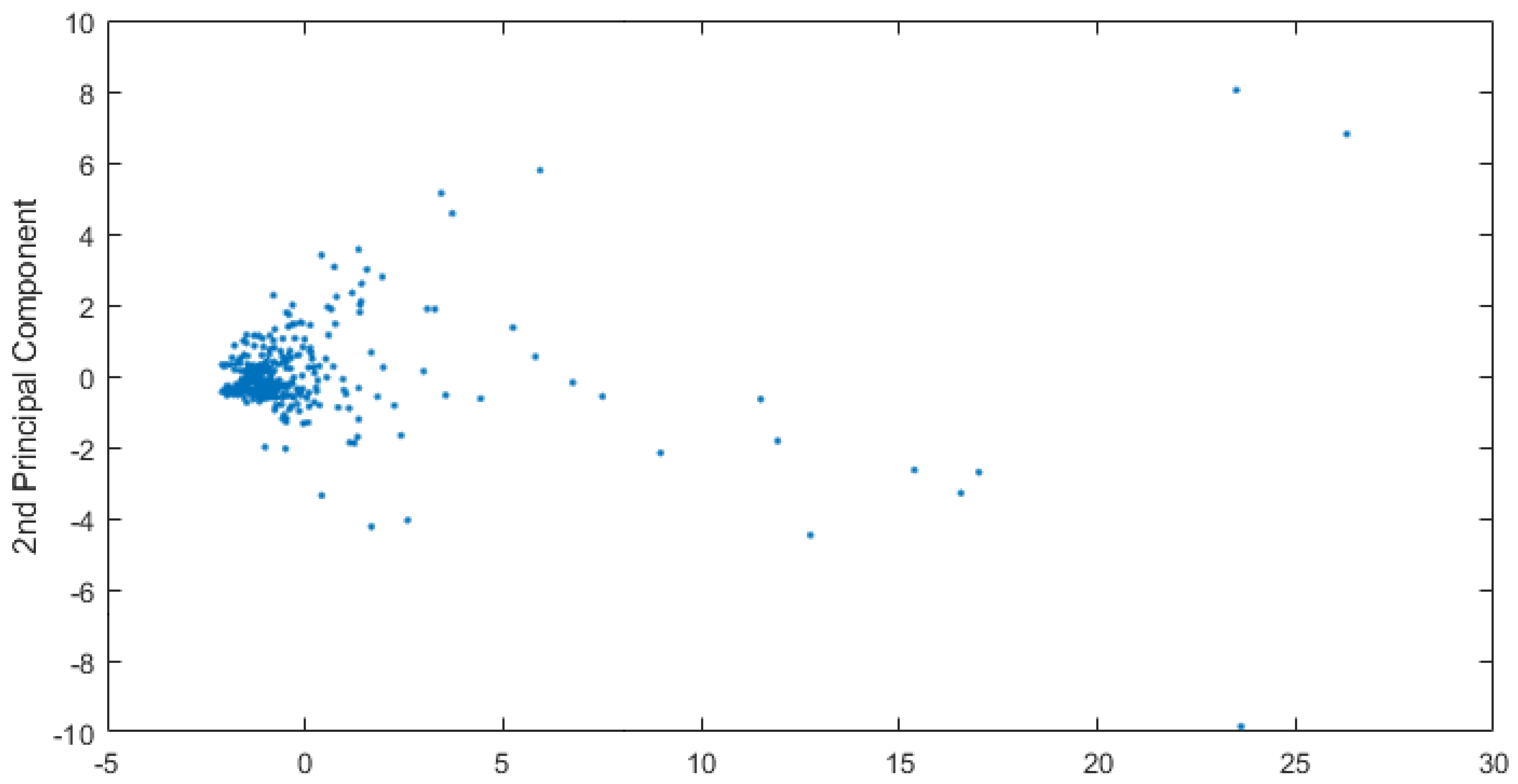
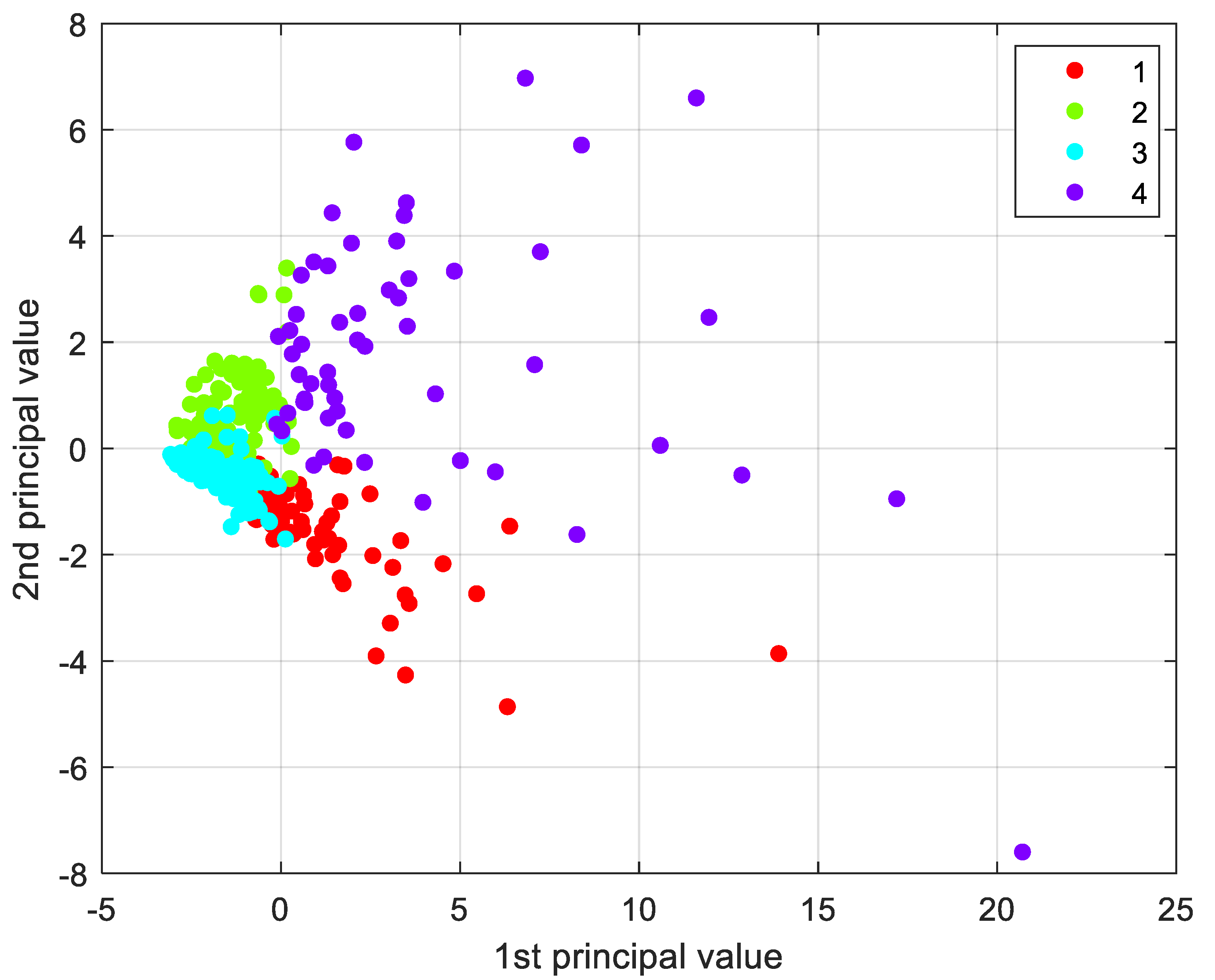
The scatter plot represented in
Figure 3, depicts the observations after variable reduction. One can notice the presence of elements defined as outliers, i.e., abnormal values, far from the average observations. These disturbing elements could generate unbalanced compensations inside the analytical model, and that is why they will be handled with care, modifying the algorithm’s settings whenever possible or, in extreme cases, removed from the dataset. In this case, the outliers were almost all the administrative centers of Emilia-Romagna region, far away, in terms of the quantitative variables, from the rest of the observations.
It is a good rule to consider the principal components that catch at least 80% of the variance of the starting dataset. The more the considered variables, the higher the number of principal components necessary to reach that quote. Whenever the amount of variance reached is not sufficient, an additional reduction in variables is performed by iterating the process.
One of PCA’s main purposes is to delete the noise due to non-useful data, which is evaluated in terms of how much information and how much variance they carry inside the dataset.
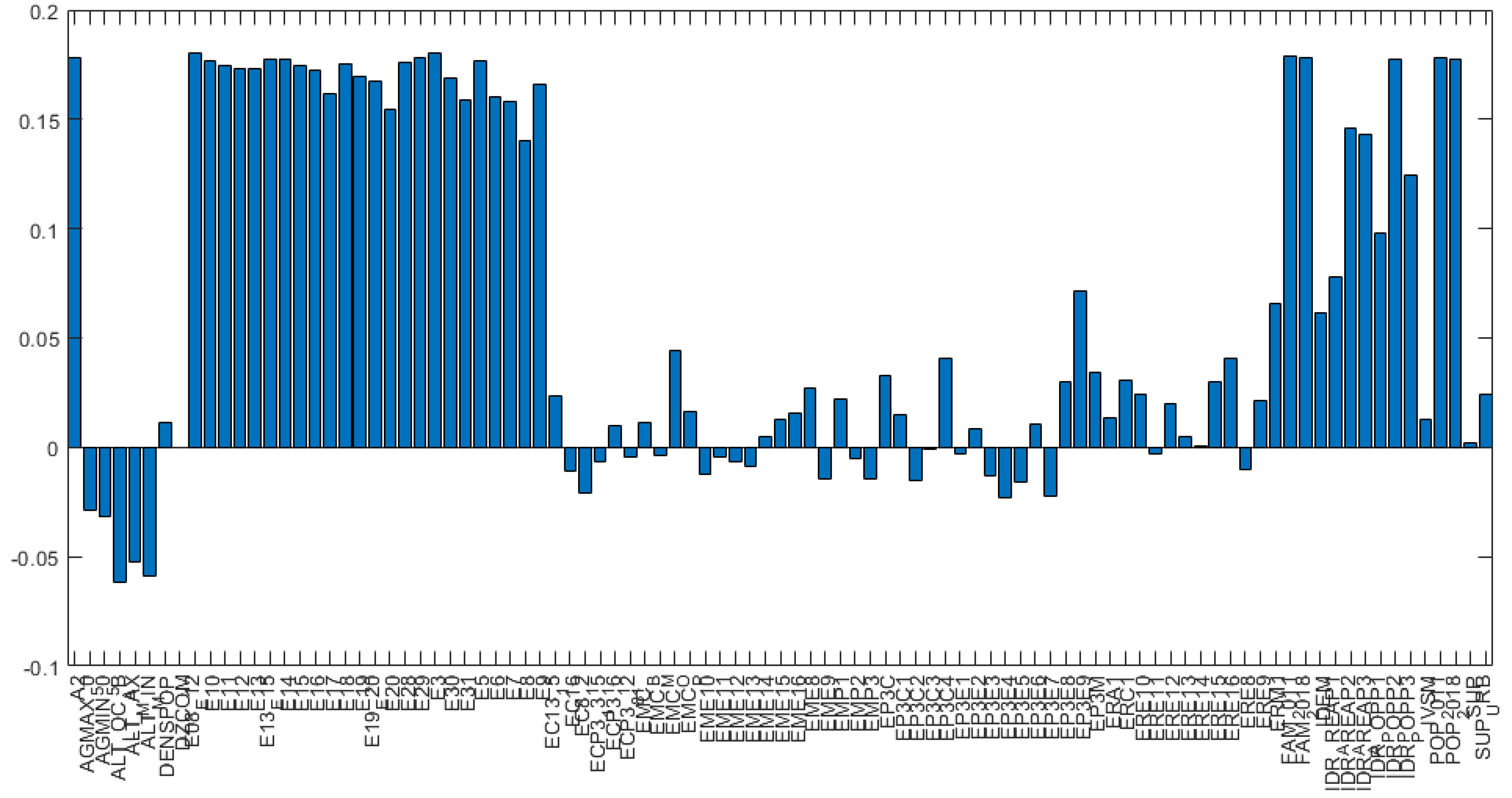
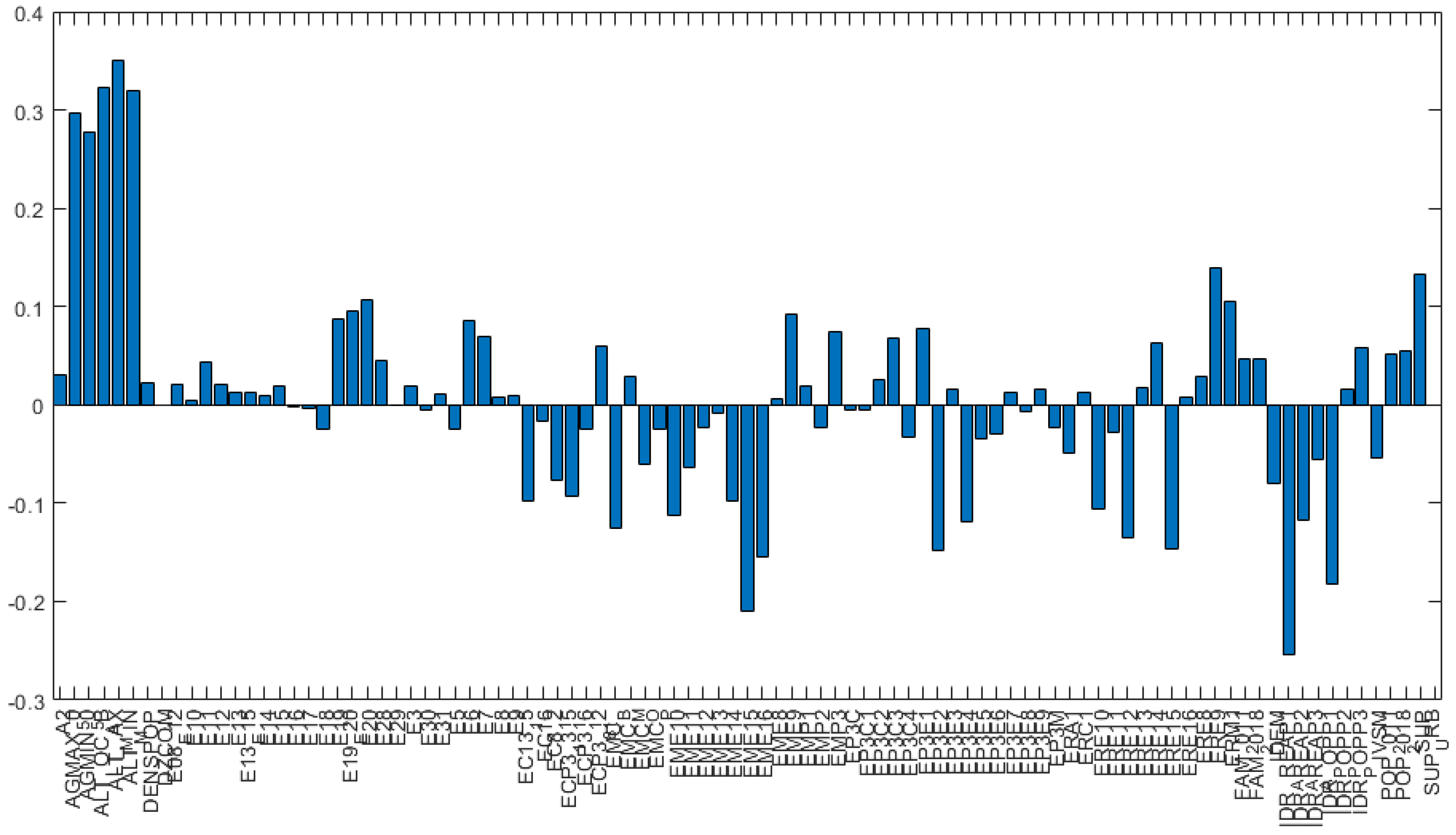
Figure 4 represents variance for each principal component before variable reduction. Loading plots have been generated as histograms representing the weight of the variables transformed after the PCA and are reported in
Figure 5 and
Figure 6. The variables reported along the abscissa have been selected among all the available data for being the most meaningful as per the multi-risk evaluation. For instance, AGMAX_50 denotes the maximum ground acceleration (fiftieth percentile) calculated on a grid with a 0.02° step, with the maximum and minimum of the values of the grid points falling within the municipal area. IDR_POPP3 indicates the resident population at risk in areas with high hydraulic hazard (P3). From
Figure 5 and
Figure 6, the variables with the highest coefficients have been extrapolated, the higher the coefficient of the variable, the higher the weight of the variable on the principal component. Along the first principal component, the difference between observations will be led by the different values referred to the variables with highest coefficient in the histogram depicted in
Figure 5.
We chose to assess the weight of the coefficient of the variables referring to the first two principal components only, because they explicated more than 70% of the variance and are the most significant of the combined risk assessment.
Figure 7 depicts the variance explicated by the first 10 principal components after the PCA.
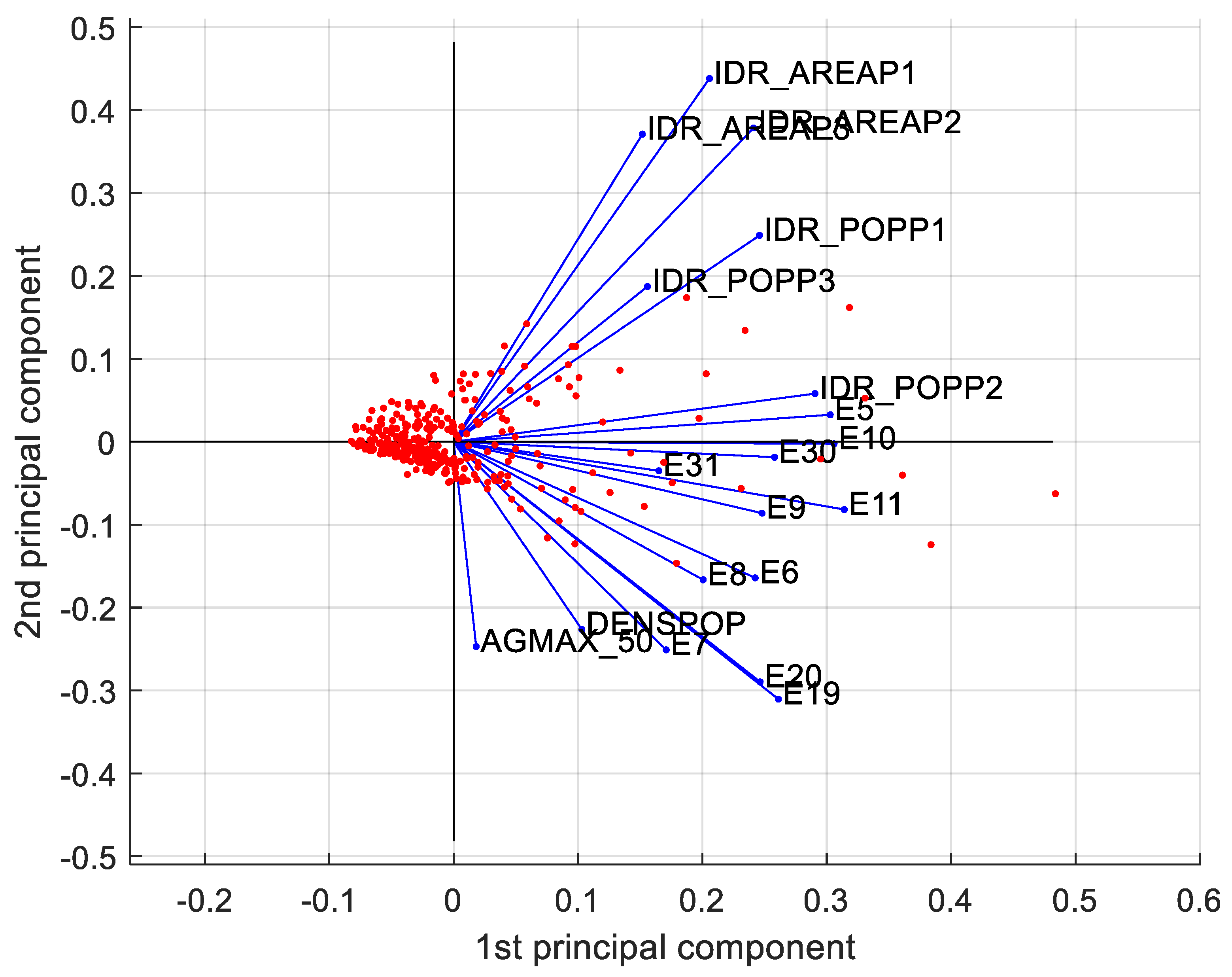
Fundamental to the visualization of both observations and the relation between the variables is the biplot in
Figure 8.
This plot allows catching at an early stage any pattern within the dataset, such as the separation between observations and deep relation among variables. In general:
the projection of the values on each principal component shows how much weight those values have on that principal component;
when two vectors are close, in terms of angle, the two represented variables have a positive correlation;
if two vectors create a 90 angle, the respective variables are not correlated;
when they diverge and create an angle of almost 180, they are negatively correlated.
Outliers differ from the other observations in terms of vulnerability and the population at hydraulic risk. It is reasonable because, remembering the outliers are the provincial administrative centers, they present higher values in terms of population and built environment. Moreover, along the vertical axis the observations differ in terms of seismic hazard and exposition.
Moreover, vulnerability and exposure to hydraulic risk variables are quite correlated and differentiate the observations along the horizontal axis, whereas seismic hazard and exposition variables are not correlated with the variables representing surfaces at hydraulic risk. These remarks will come in handy later, at a post-clustering stage, a level of multi-risk will be attributed to each cluster.

