Radio Signal Modulation Recognition Method Based on Deep Learning Model Pruning

Abstract

With the development of communication technology and the increasingly complex wireless communication channel environment, the requirements for radio modulation recognition are also increased to avoid interference and improve the efficiency of radio spectrum resources. To achieve high recognition accuracy with less computational overload, we propose a radio signal modulation recognition method based on deep learning, which uses a pruning strategy to reduce computational overload, based on the original model, CNN-LSTM-DNN (CLDNN), and the double-layer long short-term memory (LSTM). Effect factors are analyzed in terms of recognition accuracy by adjusting the parameters of each network layer. The results of the experiments show that the model not only has a greater precision improvement than some existing models, but also reduces the computational resources necessary.

1. Introduction

Today, radio technology is widely used in military, aerospace, and daily life, and plays a vital role in the transmission of information in human society. There are some unfavorable radio signals in the air that can cause serious interference with normal radio signals or may even have a significant impact on national security. Therefore, it is necessary to recognize these kinds of signals. Moreover, with the advent of the Internet of Things and the emergence of new communication technologies, wireless spectrum resources become increasingly scarce. How to identify the modulation mode, so as to judge abnormal signals in the case of channel congestion, has become a more difficult problem.

Traditional radio recognition technology usually uses a feature-based recognition method [1,2,3] and the likelihood recognition method [4,5]. The former identifies the modulation type according to the corresponding characteristics. Although the method is fast, its accuracy is low. The latter compares the received signal with the threshold to make a judgment. It is optimal in the context of Bayes, which minimizes the probability of classification error with higher accuracy, but the algorithm complexity is also higher, and cannot be used on those occasions with demanding real-time requirements. At the same time, both of the above two methods need to analyze the characteristics and parameters of the signals and then use the corresponding feature extraction function to compare and identify the modulation type. Traditional recognition methods have been unable to adapt to the current environment, so it is urgent to develop more effective and efficient identification methods.

Machine learning has become increasingly popular in recent years. Building mathematical models by modeling the neural network characteristics of human beings, after fitting large amounts of data, can predict or classify certain things in nature. Most of the available machine learning algorithms are mainly used in image recognition, natural language recognition, and speech recognition. The neural network is a type of machine learning technology that some researchers have tried to use for radio signal characteristics extraction and recognition. However, there are still problems, such as fitting and optimizing algorithms for the recognition of modulation methods in the field of radio. There are two limitations of using the convolutional neural network (CNN) model for radio modulation recognition. Firstly, if the number of network layers increases, but an improvement in recognition accuracy is not obvious, the training time load will increase [6]. Secondly, the input radio signal is a time-dependent sequence, while the image is a two-dimensional matrix, so the traditional CNN method for image recognition cannot achieve a good feature extraction effect in wireless modulation recognition. Moreover, the traditional CNN may contain many neurons or parameters that do not contribute greatly to the results. These redundant neurons may slow down the training and recognition of neural networks and may take up unnecessary hardware resources [7]. Therefore, to make our model smaller and more efficient, a pruning strategy needs to be adopted to reduce the training costs. This is particularly important for applications with a high level of real-time performance, such as radio modulation recognition, and in devices with weak computing power, such as mobile devices and edge devices.

In this paper, a pruning strategy for CLDNN [8] is proposed that greatly reduces the complexity of the model by removing unnecessary neuron nodes from the original model. The proposed method effectively improves the efficiency of radio signal modulation and reduces the risk of overfitting. Moreover, a double-layer LSTM layer is used by considering the time characteristics of the radio signal to further improve the accuracy of the radio signal modulation mode recognition. The experimental results show that the model achieves a greater precision improvement than the original model.

The rest of this paper is organized as follows. In Section 2, some related works in the literature are discussed. In Section 3 and Section 4, the analysis model and our proposed method are given. The simulation research and performance evaluation of the proposed method is presented in Section 5. Finally, the concluding remarks and future work are presented.

2. Related Work

In recent years, several studies have focused on a modulation recognition method based on CNN. The first neural network for automatic modulation recognition (AMR) was designed by O’Shea in 2016 [9]. The CNN [10] at once became the realization paradigm for AMR. After that, scholars conducted extensive research on the neural network method for AMR and designed many models to achieve the accurate recognition of modulated signals, such as long short-term memory (LSTM) [11], RseNet [12], and the convolutional long short-term memory deep neural network (CLDNN) [13]. There is no doubt that the neural network model has become an effective method for AMR.

Inspired by the AlexNet model, X. Yu et al. found that removing the full connection layer had little effect on the results [14]. They used a combination of three layers of CNN and pooled the layers, with SoftMax as an activation function, and achieved good performance. One study [15] proposed an end-to-end CNN-based automatic modulation classification (CNN-AMC) that improves accuracy through step-by-step training and improves the training speed by introducing migration learning. In [16], the authors proposed a heterogeneous depth network model based on CNN-BiLSTM, which combines CNN’s local feature with LSTM’s time characteristic. The model adopted five layers of CNN and two layers of BiLSTM (serially and in parallel). In [17], the modes are optimized, based on AlexNet, retaining the original reel layer, optimizing the parameters of the full connection layer and the pooling layer, and reducing the number of neurons. The training speed was improved and the risk of overfitting was avoided. The authors of [18] proposed deep neural networks (DNN) and a receptive field block net (RFBN), based on classification characteristics, and compared the classification performance of multiple input multiple output (MIMO) wireless modulation with K-NN, AdaBoost, and CNN networks. The authors of [19] converted complex signals into data formats (such as images) with a grid topology, as in its original application for graphics recognition, and tried to use AlexNet and GoogleNet for modulation recognition. In [20], a 34-layer CNN was designed that deepened the number of layers, showed better recognition accuracy for low signal-to-noise ratio modulation signals, and avoided under-sampling and oversampling. The authors of [21] designed a model that combined semi-supervised learning (SSL) and CNN, taking the advantages of CNN, with its high applicability, and the anti-jamming capability of SSL, with convenience and faster training speed. The authors of [22] designed a deep learning network based on a layered sparse self-encoder and SoftMax regression, which provided some performance improvement over traditional recognition methods. With the increase in complexity of the model, the computational load became very large. In [7], the authors designed a LightAMC model that made the scaling factor sparse by introducing the scale factor into the neurons and compressive sensing to help prune redundant neurons. The model size of this method was reduced by 93.5% and the calculation speed was accelerated, with a small performance loss. The authors of [23] proposed an average percentage of zeroes pruning method to reduce the network size by 37.16%, at the cost of slightly reducing the classification accuracy.

The above-mentioned works are mainly focused on research into the CNN network, and are less focused on the RNN network; some networks have too many layers, which necessitates a long training time. Thus, a model is proposed that consists of only two layers of a CNN network and two layers of an LSTM network, which represents fewer layers and less training time; we have tested it to maintain high accuracy with less training time.

In the previous works, most of them pruned the connection weights or neurons, that is, fine-grained pruning. When the weight reconnection is pruned, the network structure will become unstable, which is difficult to address in practice. The method used in this paper is layer-level pruning, which directly prunes part of the structure to improve the operation speed.

3. Problem Definition

In this paper, machine learning is used to identify the modulation of radio and to classify the input radio signals by constructing a multi-class neural network model. Inputting signal data x with a dimension size of 1 × M × N, an output of 1 × M is finally obtained, where the size of M is equal to the number of modulation types that can be classified through the network. The neural network is a reverse propagation algorithm that fits function f in y = f(x) through rounds of learning and saves the final model weight. For the newly input signal, x, the type of signal that can be obtained by this operation, and each neuron, can be represented by Equation (1):

$$z\left(x\right)=f{w}^{T}x+b$$

(1)

where $w^T$ is a T-dimensional vector representing the weight, b is a biased value, and the result z is obtained after multiple transformations by inputting the signal or the data x from the upper layer. It is then added to the SoftMax function with Equation (2):

$$p(z_i)=\frac{e^{z_i}}{{\displaystyle {\sum }_j{e}^{z_j}}}$$

(2)

where p represents the probability of the category. The loss function is of cross-entropy, which is shown in Equation (3):

$$L=-{\displaystyle \sum _{i=1}^M{y}_i\log (p_i)}$$

(3)

where M represents the number of categories, y_i represents the indicative variable (i.e., categories), and p_i represents the probability that the first category belongs to the i category.

After calculating the loss, L, the weight w and bias values b can be updated through the reverse propagation algorithm. The bias indicators of w and b can be calculated as:

$$w^{\prime }=\frac{\partial L}{\partial w}=\frac{1}{n}{\displaystyle \sum _{}^{x}x(\sigma (z)-y)}$$

(4)

$$b^{\prime }=\frac{\partial L}{\partial b}=\frac{1}{n}{\displaystyle \sum _{}^{x}x(\sigma (z)-y)}$$

(5)

where σ represents the sigmoid function and n represents the amount of training data. Therefore, a new weight and bias can be obtained, with α as the learning rate:

$$w=w-\alpha \ast w^{\prime }$$

(6)

$$b=b-\alpha \ast b^{\prime }$$

(7)

Finally, we repeat the above steps until the loss L converges and reaches a minimum value. Then, training can be stopped; the final weight is saved and can be used in the method to classify the radio modulation.

4. The Proposed Approach

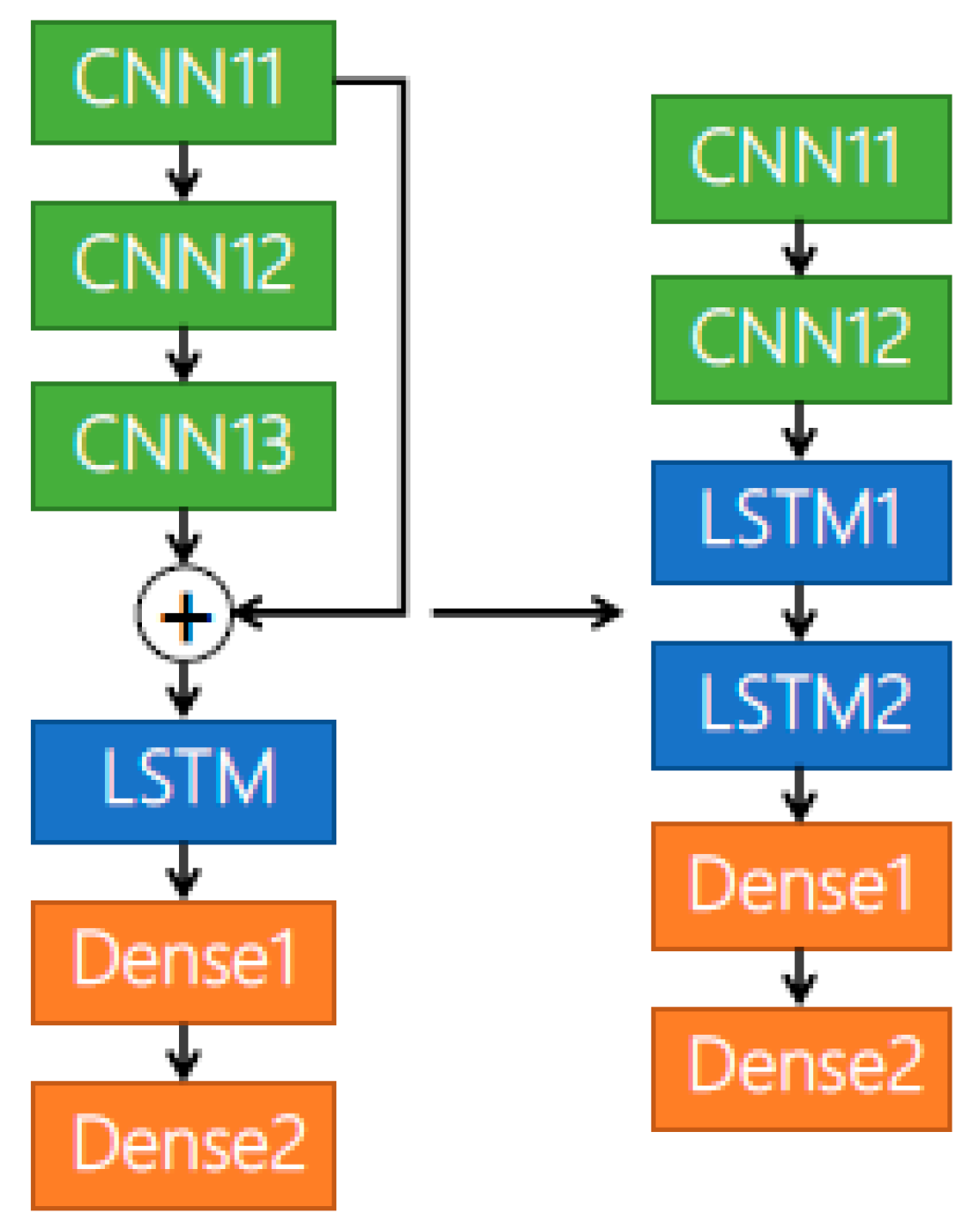
A network structure is proposed using the CNN+LSTM mode in Figure 1. When long-time series are directly processed by LSTM, the calculation requirements are very high. Therefore, a CNN is generally used to process part of the data before the use of LSTM, and the long series is replaced by the short series. The data are input to a CNN layer, are put through pooled processing, and are finally compressed to prevent overfitting. Then, batch standardization is carried out, using spatial dropout for data discarding to prevent overfitting. Then, another convolutional layer is passed, and the size of the convolutional kernel is equal to the size of the convolutional kernel of the previous convolutional layer; the boundaries are filled with zero to maintain the original size. After that, the batch standardization and pooling are carried out again; after changing the shape, the data are entered into the double-layer LSTM and are eventually classified using the full-connection layer.

Figure 1. The model structure.

LSTM is used in our model, which is mainly composed of an Input Gate, Forget Gate, Cell Update, and Output Gate. The structure of LSTM is shown in Figure 2.

Figure 2. LSTM structure.

These gates’ functions are explained below.

Input Gate: This controls how much of the current input x_t and the previous output h_t-1 will be entered into the new cell:

$$i_t=\sigma (W_i{x}_t+U_i{h}_{t-1}+b_i)$$

(8)

where i_t is the output of the input gate, W_i and U_i are the weights of the input gate, b_i is the bias of the input gate, x_i is the input of this cell, and h_t−1 is the output of the last cell.

Forget Gate: This decides whether to erase (set to zero) or to keep individual components of the memory:

$$f_t=\sigma (W_f{x}_t+U_f{h}_{t-1}+b_f)$$

(9)

where f_t is the output of the forget gate, W_f and U_f are the weights of the forget gate, and b_f is the bias of the forget gate.

Cell Update: This transforms the input and previous state to be considered into the current state:

$${\tilde{c}}_t=\tanh (W_c{x}_t+U_c{h}_{t-1}+b_c)$$

(10)

where ${\tilde{c}}_t$ is the candidate cell state, W_c and U_c are the weights of the forget gate, and b_c is the bias of the forget gate.

Output Gate: This scales the output from the cell:

$$o_t=\sigma (W_o{x}_t+U_o{h}_{t-1}+b_o)$$

(11)

where o_t is the output coefficient of this cell, W_o and U_o are the weights of the output gate, and b_o is a bias of the output gate.

Internal State update: This computes the current time step’s state using the gated previous state and the gated input:

$$c_t={\tilde{c}}_t\cdot i_t+c_{t-1}\cdot f_t$$

(12)

where c_t is the cell status.

Hidden layer: the output of the LSTM, scaled by a tanh (squashed) transformation of the current state:

$$h_t=o_t\cdot \tanh (c_t)$$

(13)

where h_t is the output of this cell.

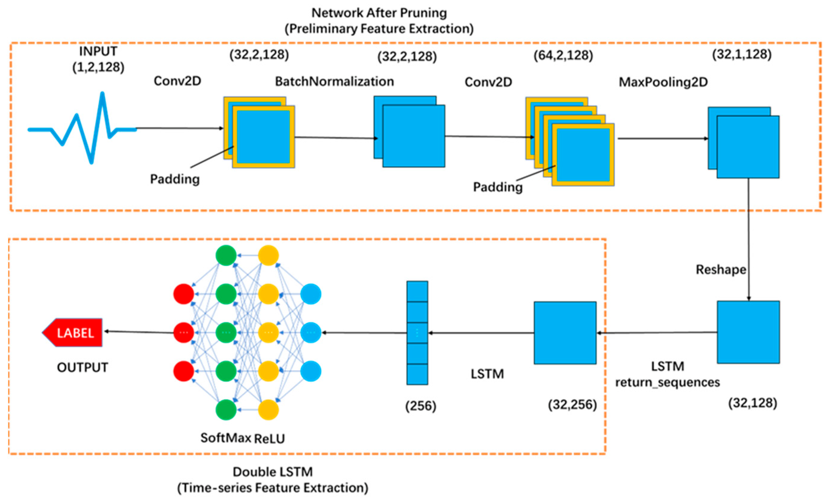
The accuracy of the results is improved by removing the third CNN layer, combining the first and second layers of CNN, and adding a layer of the LSTM layer. The pruning process is shown in Figure 3.

Figure 3. The pruning model structure.

In the CNN module, after convolution and pooling, the data features are reconstructed and input into the LSTM unit. At this point, the data comprise 32 feature maps, each of which includes 128 feature values. After being processed by the first LSTM unit, the data become a second-order vector composed of 32 timestamps, each of which contains 256 features. The first layer uses the LSTM unit to further extract the features extracted from the convolution layer. The role of LSTM in the second layer is to reduce the dimension of the time steps of the data and compress all features into a timestamp; the output at this time is 256 feature values, which can be directly sent to the classification layer for classification.

We pruned the convolution layer that needs a convolution operation and realized the data reconstruction by adding an LSTM layer. This has the advantage of reducing the amount of calculation required for convolution operation and of saving more data features for the LSTM layer operation.

5. Experimental Analysis

The simulation tool for our experiment is Keras 2.0, based on Linux. The batch size is set to 256. The optimizer is Adam, and the learning rate remains Keras’ default value. The maximum number of epochs is set to 100. The hardware uses an NVidia Tesla P4 (8 GB memory) GPU, with 12 GB of memory. All the data are calculated by testing three times to average it, and the loss value is calculated. The effects of five parameters on the proposed model are shown and discussed below. Our model is also compared with some of the existing models as well.

5.1. The Effect of CNN Kernel Size

The effect of CNN kernel size was first studied. The experimental results are shown in Figure 4. It can be seen that the kernel size of the CNN layer is positively related to the accuracy; that is, the larger the CNN kernel size, the better the result.

Figure 4. The impact of the size of the CNN kernel on classification accuracy.

However, with the large kernel size, the training time will be increased, and the verification set will become unstable and unable to converge, so the best CNN kernel size is set to 4 × 4, as shown in Table 1.

Table 1. The impact of the size of the CNN kernel on classification accuracy.

Kernel Size	Loss
1 × 2	1.2986183166503906
1 × 3	1.2517382701237996
1 × 4	1.2592326800028484
1 × 5	1.1835391124089558
2 × 2	1.1842063665390015
2 × 3	1.1451027790705364
2 × 4	1.1322169701258342
2 × 5	1.1263486941655476
3 × 3	1.1229949394861858
4 × 4	1.1136138439178467

5.2. The Effect of LSTM Unit Size

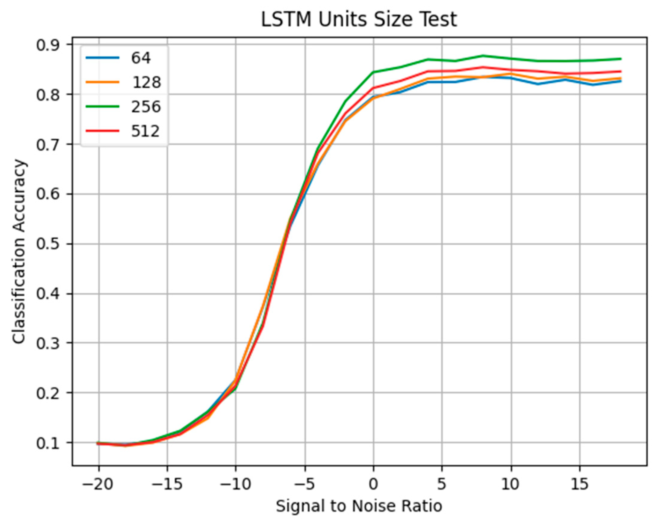
In Figure 5, it can be seen the larger the LSTM unit size, the higher the classification accuracy. When the size of LTSM has been doubled, the recognition accuracy is improved. However, with the increase in LTSM size, the training time has also increased. Therefore, the best trade-off of 256 is selected.

Figure 5. The impact of the size of the LSTM unit on classification accuracy.

5.3. The Effect of LSTM Layer Number

The accuracy will improve by adding LSTM layers. In Figure 6, it can be seen that the two-tier LSTM network has about a 3% accuracy improvement, compared to the one-layer network. After continuing to increase the number of LSTM layers, the results do not change a great deal, so the two-layer LSTM is set.

Figure 6. The impact of the LSTM layer number on classification accuracy.

5.4. The Effect of Dropout Layer Type

After using the second layer of the LSTM layers, the loss at first falls very quickly, and the accuracy is then much better than that of the single-layer LSTM. However, after the 10th epoch, the accuracy improves slowly, and gradually trends toward overfitting, resulting in an increase in the loss.

When using an ordinary dropout, the loss will fall slowly along with the increase in the forgetting rate; while the accuracy will decrease, the accuracy will also decline. However, there will be overfitting along with the decrease in the forgetting rate, which causes loss jitter.

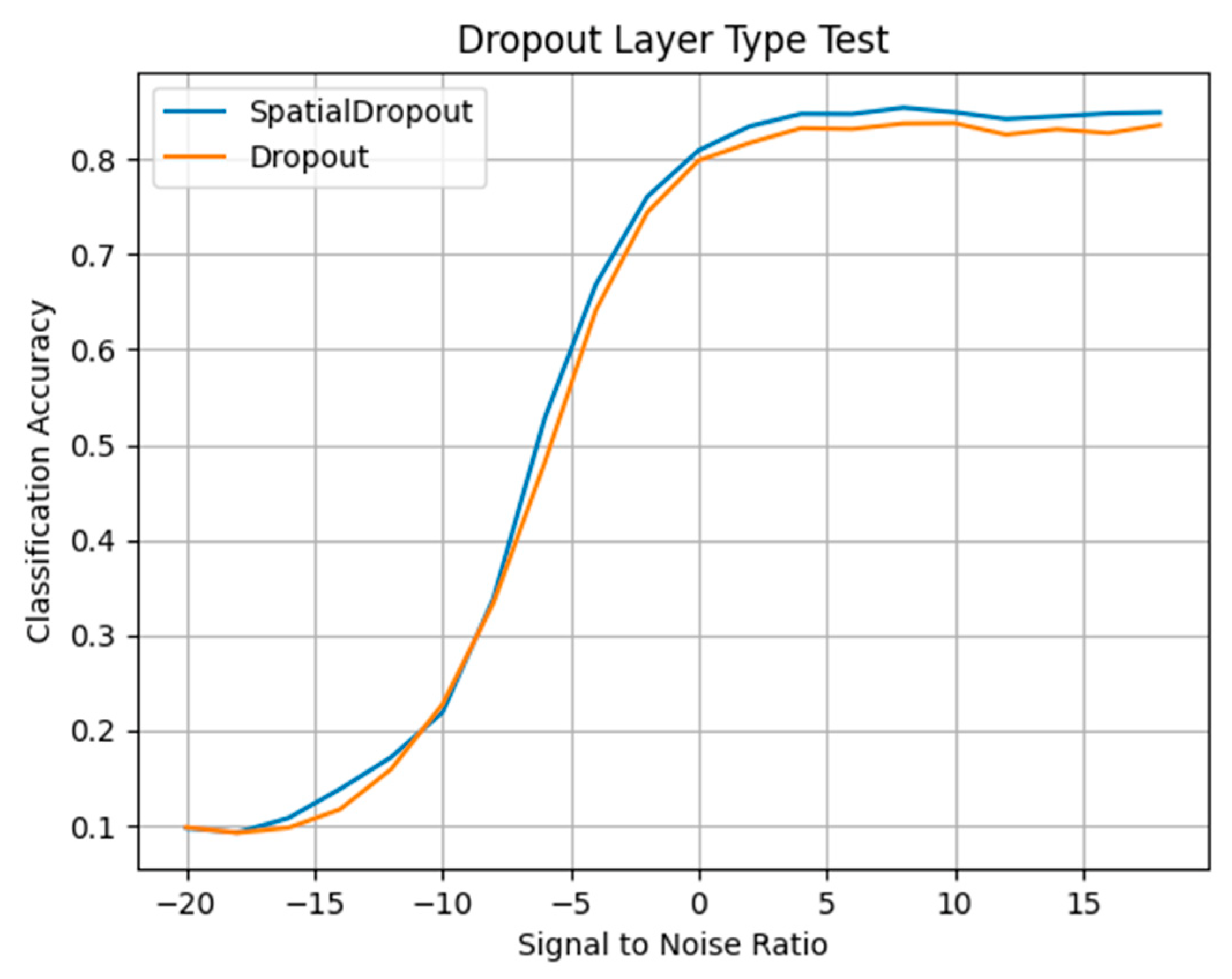
To solve this problem, the Spatial Dropout is used instead of the ordinary Dropout. As can be seen from Figure 7, the accuracy is thereby improved by about 3%.

Figure 7. The classification accuracy of Spatial Dropout and ordinary Dropout.

5.5. The Effect of Batch Size

It can be seen from Figure 8 and Table 2 that with the increase in batch size, the training time decreases gradually, but the recognition accuracy reaches the maximum when the batch size = 256.

Figure 8. The impact of the batch size on classification accuracy.

Table 2. The impact of the size of the batch size on classification accuracy.

Batch Size	Loss	Time Per Epoch (s)
64	1.153881827990214	26
128	1.1463038523991902	17
256	1.119464596112569	13
512	1.1418431202570598	11
1024	1.1403136253356934	9
2048	1.1303218603134155	8

As can be seen from the results, with the 256 batch size, each epoch of training time and loss can achieve a better result, so the model chose to use 256 as the value of Batch size.

5.6. Comparison with Existing Models

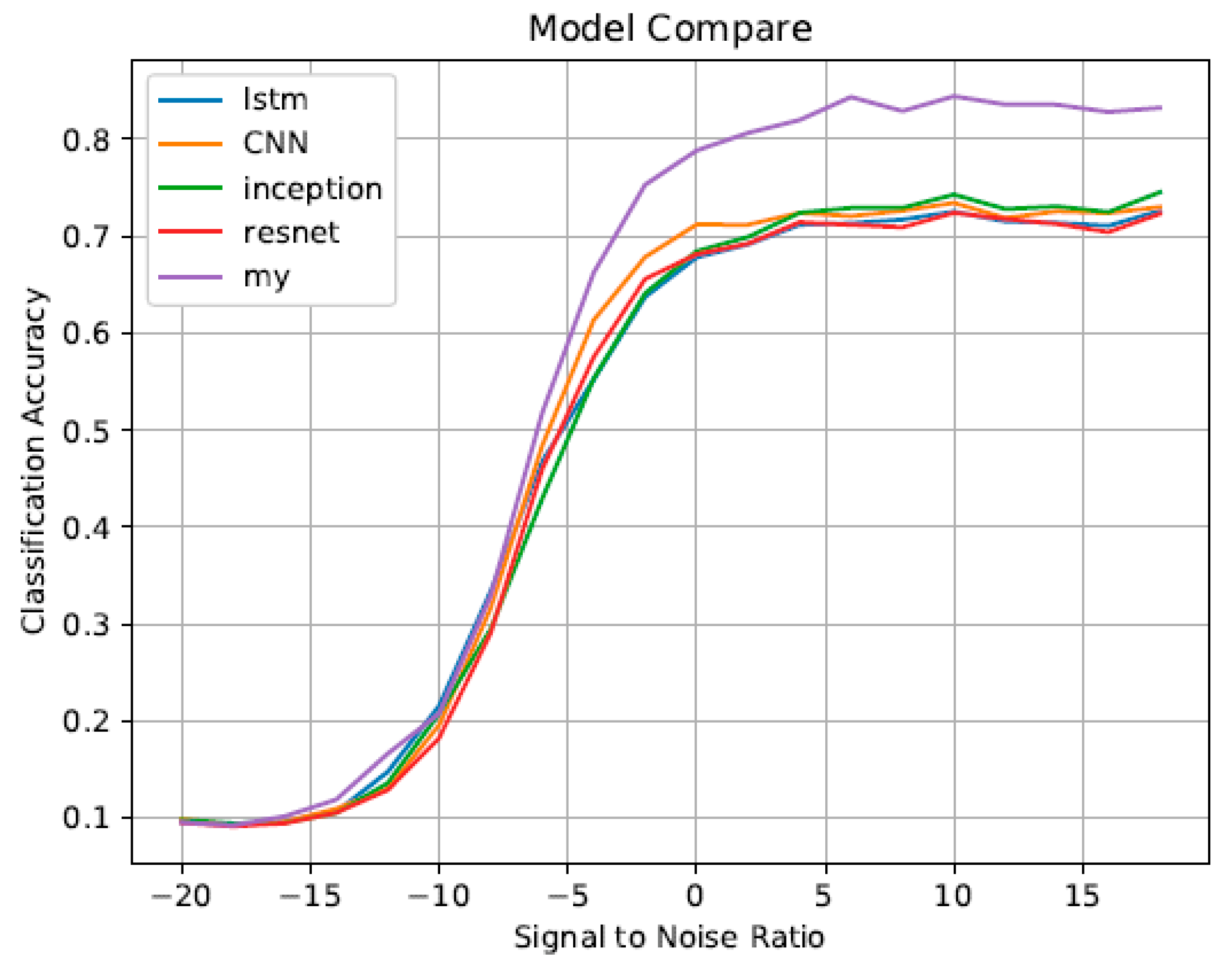
The proposed scheme is compared with some existing models by using the experiment parameters above in Figure 9 to evaluate its performance. Among them, the prediction effect of LSTM is the worst because the single LSTM model cannot effectively extract local features, and the increase in the number of neurons leads to an increase in calculation quantity and the risk of overfitting.

Figure 9. Comparison of the classification accuracy with the existing models.

Our proposed model has higher recognition accuracy than the other existing models under different SNR conditions. Compared with CNN and LSTM, the CNN-LSTM model with pruning improves the recognition accuracy by more than 10% under 0 dB and higher SNR. These improvements are mainly because the radio signal is a time-related sequence, so the LSTM layer number and unit size to the appropriate state can be adjusted to achieve better accuracy. Moreover, pruning technology is used to reduce the amount of computation, so that the model can be trained faster without reducing its accuracy.

6. Conclusions

To overcome the problems of low efficiency, high cost, and the low recognition rate of existing radio recognition through deep learning, a CNN-LSTM-DNN model is proposed. The pruning strategy of the CLDNN model is first used, which greatly reduces the complexity of the model and reduces the risk of overfitting, by removing unnecessary neuron nodes from the original model. Then the double-layer LSTM is employed by considering the time characteristics of the radio signals, to further improve the accuracy of modulation mode recognition

Throughout the experiments to adjust the parameters of each layer to a better value, the model in the training time slightly increases the accuracy of the results. In comparison with previous research [6], our model training results can be about 10% more accurate than the original model. As the neurons, connections between layers, and weights are reduced, there is a reduction in storage requirement and heat dissipation in deployed hardware, which can be used in embedded devices with limited hardware resources.

In our future works, we will select the compression methods and the pruning strategy according to the architecture of specifically targeted hardware to reduce the inference time and memory constraints.

References

1. Dobre, O.A.; Abdi, A.; Bar-Ness, Y.; Su, W. The classification of joint analog and digital modulations. In Proceedings of the MILCOM 2005—2005 IEEE Military Communications Conference, Atlantic City, NJ, USA, 17–20 October 2005. [Google Scholar] [CrossRef]
2. Hazza, A.; Shoaib, M.; Alshebeili, S.A.; Fahad, A. An overview of feature-based methods for digital modulation classification. In Proceedings of the 2013 1st International Conference on Communications, Signal Processing and their Applications (ICCSPA), Sharjah, United Arab Emirates, 12–14 February 2013. [Google Scholar] [CrossRef]
3. Yu, Z.; Shi, Y.Q.; Su, W. M-ary frequency shift keying signal classification based-on discrete Fourier transform. In Proceedings of the IEEE Military Communications Conference, Boston, MA, USA, 13–16 October 2003. [Google Scholar] [CrossRef]
4. Sills, J.A. Maximum-likelihood modulation classification for PSK/QAM. In Proceedings of the MILCOM 1999 IEEE Military Communications Conference Proceedings, Atlantic City, MA, USA, 31 October—3 November 1999. [Google Scholar] [CrossRef]
5. Lin, Y.C.; Kuo, C. Sequential modulation classification of dependent samples. In Proceedings of the 1996 IEEE International Conference on Acoustics, Speech and Signal Processing Conference Proceedings, Atlanta, GA, USA, 9 May 1996. [Google Scholar] [CrossRef]
6. Chen, S.; Zhang, Y.; He, Z.; Nie, J.; Zhang, W. A novel attention cooperative framework for automatic modulation recognition. IEEE Access 2020, 8, 15673–15686. [Google Scholar] [CrossRef]
7. Wang, Y.; Yang, J.; Liu, M.; Gui, G. LightAMC: Lightweight automatic modulation classification via deep learning and compressive sensing. IEEE Trans. Veh. Technol. 2020, 69, 3491–3495. [Google Scholar] [CrossRef]
8. West, N.E.; O’Shea, T.J. Deep architectures for modulation recognition. In Proceedings of the 2017 IEEE International Symposium on Dynamic Spectrum Access Networks (DySPAN), Baltimore, MA, USA, 6–9 March 2017. [Google Scholar] [CrossRef]
9. O’Shea, T.J.; Corgan, J.; Clancy, T.C. Convolutional radio modulation recognition networks. In Proceedings of the International Conference on Engineering Applications of Neural Networks, Aberdeen, UK, 19 August 2016. [Google Scholar] [CrossRef]
10. Huynh-The, T.; Hua, C.H.; Pham, Q.V.; Kim, D.S. MCNet: An efficient CNN architecture for robust automatic modulation classification. IEEE Commun. Lett. 2020, 24, 811–815. [Google Scholar] [CrossRef]
11. Zhang, Z.; Luo, H.; Wang, C.; Gan, C.; Xiang, Y. Automatic modulation classification using CNN-LSTM based dual-stream structure. IEEE Trans. Veh. Technol. 2020, 69, 13521–13531. [Google Scholar] [CrossRef]
12. Zhang, H.; Yuan, L.; Wu, G.; Zhou, F.; Wu, Q. Automatic modulation classification using involution enabled residual networks. IEEE Wirel. Commun. Lett. 2021, 10, 2417–2420. [Google Scholar] [CrossRef]
13. Ramjee, S.; Ju, S.; Yang, D.; Liu, X.; Gamal, A.E.; Eldar, Y.C. Fast deep learning for automatic modulation classification. arXiv 2019, arXiv:1901.05850. https://arxiv.org/abs/1901.05850. [Google Scholar]
14. Yu, X.; Li, D.; Wang, Z.; Guo, Q.; Wei, X. A deep learning method based on convolutional neural network for automatic modulation classification of wireless signals. Wirel. Netw. 2019, 25, 3735–3746. [Google Scholar] [CrossRef]
15. Fan, M.; Peng, C.; Wu, L.; Wang, X. Automatic modulation classification: A deep learning enabled approach. IEEE Trans. Veh. Technol. 2018, 67, 10760–10772. [Google Scholar] [CrossRef]
16. Zhang, D.; Ding, W.; Zhang, B.; Xie, C.; Li, H. Automatic modulation classification based on deep learning for unmanned aerial vehicles. Sensors 2018, 18, 924. [Google Scholar] [CrossRef] [PubMed]
17. Zhu, L.; Gao, Z.; Zhu, Z. Blind Modulation Classification via Accelerated Deep Learning. In Proceedings of the 2019 IEEE 5th International Conference on Computer and Communications (ICCC), Chengdu, China, 6–9 December 2019. [Google Scholar] [CrossRef]
18. Shah, M.H.; Dang, X. Low-complexity deep learning and rbfn architectures for modulation classification of space-time block-code (stbc)-mimo systems. Digit. Signal Process. 2020, 99, 102656. [Google Scholar] [CrossRef]
19. Peng, S.; Jiang, H.; Wang, H.; Alwageed, H.; Yao, Y.D. Modulation classification based on signal constellation diagrams and deep learning. IEEE Trans. Neural Netw. Learn. Syst. 2018, 99, 1–10. [Google Scholar] [CrossRef] [PubMed]
20. Guo, J.; Zhang, H.; Xu, J.; Chen, Z. Pattern Recognition of Wireless Modulation Signals Based on Deep Learning. In Proceedings of the 2019 IEEE 6th International Symposium on Electromagnetic Compatibility (ISEMC), Nanjing, China, 1–4 November 2019. [Google Scholar] [CrossRef]
21. He, X.; Lin, L.; Xie, J. Recognition of Signal Modulation Mode Based on Gaussian Filter and Deep Learning. In Proceedings of the 2018 3rd International Conference on Computer Science and Information Engineering (ICCSIE 2018), Xian, China, 21 September 2018. [Google Scholar] [CrossRef]
22. Li, J.; Lin, Q.; Yun, L. Research on modulation identification of digital signals based on deep learning. In Proceedings of the 2016 IEEE International Conference on Electronic Information and Communication Technology (ICEICT), Harbin, China, 20–22 August 2016. [Google Scholar] [CrossRef]
23. Zhang, Z.; Tu, Y. A Pruning Neural Network for Automatic Modulation Classification. In Proceedings of the 2021 8th International Conference on Dependable Systems and Their Applications (DSA), Yinchuan, China, 5–6 August 2021. [Google Scholar] [CrossRef]
Publisher’s Note: MDPI stays neutral with regard to jurisdictional claims in published maps and institutional affiliations.
Article Metrics
Citations
Article Access Statistics
Multiple requests from the same IP address are counted as one view.