Multi-Feature Extraction-Based Defect Recognition of Foundation Pile under Layered Soil Condition Using Convolutional Neural Network

Abstract

If the layer of soil surrounding a pile is not taken into account during the engineering detection process, the velocity-time curve might show asymptotic diameter shrinkage or diameter expanding features, which would alter the interpretation of the test findings. In this study, we suggest combining multi-feature extraction and a convolutional neural network (CNN) to increase accuracy in pile defect recognition for layered soil conditions and traditional deep learning flaws. First, numerical simulations are run to create velocity–time curves for foundation piles under layered soil conditions. Then, the data are extracted from three dimensions: time domain, frequency domain, and time-frequency domain, respectively, and fused into a set of feature vectors. Finally, a foundation pile defect identification model combining multi-scale features and CNN is established. The findings demonstrate that the CNN model has 97.8% accuracy while the PNN has 28.6% accuracy, demonstrating that the approach is very reliable.

1. Introduction

Pile foundations, as load-bearing elements supporting superstructures, often display strong load-bearing capacity under various challenging engineering and geological circumstances. Pile fracture, expansion, shrinkage, segregation, and other problems are frequently brought on by subpar construction technology, a complex geological environment, a limited level of construction personnel, and other factors. This makes pile foundation engineering a project that is difficult to control. These issues are directly connected to people’s lives and property safety. Foundation pile quality checking is a crucial step in reducing engineering hazards. After years of development, the low strain reflection wave method has become an efficient tool for engineering the examination of pile integrity due to its straightforward equipment, lightweight, low cost, and accurate and dependable test findings [1].

The low-strain reflection approach involves detecting and analyzing stress waves using sensors. The reflection and transmission of the stress waves occur when the impedance of the cross section changes during propagation. The integrity of the foundation pile is judged by analyzing and processing the stress reflected wave signal. Signal processing and signal feature extraction are essential to determine the accuracy of subsequent pile foundation detection classification and recognition. Wavelet analysis is very effective for the local feature analysis of the signal [2], but the nature of the signal in other time and frequency domains is not fully considered. Moreover, the wavelet transform is very dependent on the wavelet basis function and the decomposition level, and there is a great deal of artificiality in selecting the basis function. Many scholars have selected the wavelet basis function with a stroke [3,4,5]. The same signal uses different wavelet basis functions to decompose. It will have different effects, which directly affect the discriminant effect of the dynamic signal and result in a reduction in the method’s practicality. Several Intrinsic Mode Functions (IMF) are directly separated from the signal using the Empirical Mode Decomposition (EMD) technique [6]. The fact that each IMF is orthogonal to the others is essential. Nevertheless, the only drawback is that modal aliasing occurs quickly in decomposition. Ensemble Empirical Mode Decomposition (EEMD) is an excellent solution to the phenomenon of mode mixing. In 2009, Zhaohua Wu et al. [7] from Florida State University added white noise to EMD. However, it is necessary to set the white noise amplitude and the number of iterations artificially, which results in significant reconstruction errors and poor decomposition completeness. To overcome the reconstruction inaccuracy, Torres et al. [8] developed an entire ensemble empirical mode decomposition with adaptive noise (CEEMDAN). White noise then embraces the signal using the original EEMD approach, effectively reducing the model complexity. However, CEEMDAN still produces a small number of faulty components and residual noise in the decomposition process. Therefore, Colominas et al. [9] proposed an Improved CEEMDAN (ICEEMDAN) in 2014. Based on CEEMDAN, the signal is continually divided by adding Gaussian white noise, and the resulting signal is averaged. In contrast to the CEEMDAN signal decomposition technique, this method dramatically inhibits the phenomenon of faulty components in signal decomposition and effectively improves the efficiency of signal decomposition.

All of the above signal processing methods could successfully capture the signal’s features, and some professors have researched the extraction of eigenvalues. Cai, Q.Y. [10] used multi-resolution analysis to capture the feature vector representing the power spectrum’s power composition fed into a neural network to identify the pile defect. To obtain the energy mean and power spectrum in the frequency range as feature vectors to input into the neural network, Bai, Q.L. [11] employed wavelet transform. Jiang, X.L. [12] selected Daubechies4 wavelet 5-layer multi-resolution analysis to extract the characteristic frequency spectrum amplitude. In 2015, Kang, W.X. and Li, J.D. [13] of the Harbin Institute of Technology proposed for the first time that quantized information entropy could be used to detect stress wave signals, and the quantized information entropy was proved to be very comprehensive after experiments. Li, J.D. [14] built a feature vector using quantized information entropy, energy, and variance utilizing the wavelet package calculation. The results revealed that the feature is helpful for stress wave signal singularity detection. From the above studies, it can be concluded that in the processing of foundation pile dynamic measurement signals, the feature values extracted are all from the same dimension, mostly variance, power spectrum means, and information entropy, which does not differentiate enough between defects. However, the defect information in the foundation pile detection signal under layered soil conditions is very complex and rich. It is often insufficient to characterize the complex signal with only one-dimensional features, so a more in-depth study is needed in extracted features.

Machine learning is frequently utilized in defect recognition as science and technology advance. Support vector machines are well suited to the learning method for small sample situations, cleverly solving the dimensionality problem and avoiding dimensional disasters. Kang, W.X. [15], Li, Z.B. [16], and Xue, Z.J. [17] used support vector machines to identify the type and degree of foundation pile defects based on the minor sample nature of the test data, which improved the accuracy of the classification of foundation pile defects. Deep learning is also advancing quickly, and neural networks, with their strong self-learning and nonlinear mapping capabilities, are particularly suitable for recognizing complex signals. Good results have been achieved in recognizing foundation pile defects [18,19].

It is challenging to show during foundation pile integrity testing when the engineering properties of the soil on the pile side change significantly whether the characteristic signals on the curve are brought on by pile defects or geological changes simply based on the reflected wave curve in the field [20]. To avoid the interference of soil formation on the foundation pile integrity and improve the inspectors’ efficiency, this paper analyses the changing pattern and characteristics of the dynamic measurement curve of the pile body with common defects by establishing a three-dimensional finite element model and verifies the numerical simulation using experiments. The article combines multi-feature extraction and a convolutional neural network to achieve an accuracy of 97.8% in recognizing foundation pile defects, which realizes the automated detection of foundation pile defects.

The quality problem of foundation pile engineering will involve various aspects. Consequently, the state places a high value on the quality inspection department; yet, due to testing expenses and project progress limitations, the quality inspection department usually uses random inspections to control the quality of the project. Random inspection results tend to miss some defective foundation piles, and the inspection results lack impartiality. It is essential to research and explore methods for testing foundation piles at a lower cost and a higher level of inspection. Therefore, this research has good theoretical and practical application value and is highly important in terms of both societal and economic rewards.

2. Materials and Methods

2.1. Theoretical Basis of Pile Detection by Low Strain Reflection Wave Method

When pile length L > > pile diameter D, the stress wave length λ > > D conforms to the setting of the one-dimensional rod, and the stress wave’s progression in the pile will be calculated using the one-dimensional rod fluctuation equation. When there are defects in the pile, the wave will produce reflection and transmission; reflected waves propagate reverse along the pile to the top of the pile; the transmitted wave continues to propagate downward. Using the characteristic line method to solve the fluctuation equation, you can obtain the velocity reflected wave and transmission wave at the interface of the pile body defects and the incident wave [21]:

$$V_r=V_i\cdot \frac{1-\beta }{1+\beta }$$

(1)

$$V_t=V_i\cdot \frac{2}{1+\beta }$$

(2)

The essential physical features of the incident wave, reflecting wave, and transmit wave are represented by the subscript symbols i, r, and t. Pile integrity coefficient β = Z₂/Z₁, impedance Z = ρAC; ρ is the pile density; A represents the pile’s cross-sectional area; $\mathrm{C}=\sqrt{\mathrm{E}/\mathsf{\rho }}$ is the velocity of stress wave transmission in the pile body.

2.2. Numerical Simulation of Dynamic Test of Foundation Pile in Layered Soil

In machine learning classification, a large amount of data is needed to train and learn the classification model. It is not easy to collect dynamic test data of defective piles in engineering, and it is impossible to obtain abundant data on defective piles through experiments only. Abaqus enables the simulation of common problems in engineering. The contact problem is a smooth nonlinear problem. The display product approach in Abaqus is more appropriate for handling the stress wave propagation problem because there is no relative displacement between them [22]. Nevertheless, the actual test pile experiment is expensive in the actual study, and the defective pile cannot be used in the actual project after the test. Therefore, to minimize the experiment’s cost, this study was carried out to obtain the dynamic test curve data of the foundation pile under layered soil conditions through finite element simulation.

2.2.1. Basic Theory and Model Establishment

First, select the component module and set the model space, type, and essential characteristics via the component manager. Reducing the impact of reflected waves on the numerical simulation results after the stress waves have propagated to the soil boundary. There are two general methods of setting up the finite element calculation; one is to set up absorbing boundary conditions such as viscoelastic boundaries, and the other is to set up a wide range of soil boundaries. In this paper, we set a wide range of soil boundaries for consistency and clarity of computation. The selection of the geometric model of the soil unit on the side of the pile is one of the vital factors affecting the calculation’s outcomes. The model is not as large as it should be, as the calculation time increases significantly due to the large model. In the foundation piles, a finite element simulation, the area of clay around the pile that Tanchanis utilized was 1.4 times the length and 12 times the diameter of the pile. The analysis showed that it was sufficient to evaluate the piling foundation’s carrying capability [23]. The American Petroleum Institute believes that the lateral soil within the range of 8D will impact the pile foundation’s bearing capacity [24]. Cooke obtained from the analysis of the experimental data of London clay that when the measured minimum pile spacing was 12D, the two piles would not affect each other. For a single pile, 6D was sufficient. When the soil radius there was roughly 10D, the shear displacement was essentially small [25].

Based on the above research, the diameter of the pile–soil model is 10 times the pile diameter, the depth direction is 1.5 times the pile length, and the pile is 1 m long and has a 0.1 m diameter. Figure 1 depicts a model of the pile and soil.

The characteristics of the segment and the material. When the pile is tested under low strain, the deformation caused by the excitation force of the pile is minimal. The deformation stage assumes that the pile is in the linear elastic deformation stage; thus, linear elasticity is the description of the material model. To make the model simple and effective, it is assumed that the soil beneath the pile and the surrounding area is also linear elastic [26]. The material attribute element simulates the segregation part with a lower elastic modulus than the pile body, and the fractured part is simulated by the air element [27]. The selection of pile–soil material parameters comes from study 27 [28]. The specific numbers can be seen in

Table 1. Pile–soil material parameters.

Part	Elastic Modulus E(GPa)	Density ρ(kg/m3)	Poisson Ratio ν	Friction Coefficient fs
pile	30	2400	0.17	-
soil layer 1	0.015	1930	0.32	0.5
soil layer 2	10	2250	0.25	0.6
segregation part	15	2000	0.23	-
breakdown part	1.293	0	0	-

.

Define assembly. The function of the assembly is to assemble the parts to form an analysis.

We are setting the analysis step. Because the analysis step completes the simulation process, the analysis step is determined by the requirements. Therefore, 2 L/C = 0.0006 s is the analysis step length, and the analysis step time is 0.0008 s. By setting the historical output to replace the sensor, the output point of the signal is set at the position of 2/3 R at the pile top.

Establish interaction rules. The contact with the soil around the pile is face-to-face contact, and the rubbing is in the form of a penalty. The friction coefficient between the pile and each layer of soil is f_s, and the contact between the pile bottom and the soil at the pile bottom is set as the binding constraint [29].

Determining the bounds and the loading. The longitudinal transient exciting force at pile top can be simulated by using the rising chord pulse function (formula 3) well in line with the actual testing exciting force [26]:

$$p\left(t\right)=\frac{I}{T_d}\left(1-\cos \frac{2\pi }{T_d}t\right)\begin{array}{cccc}& & 0\le t\le T_d& \end{array}$$

(3)

T_d and I represent the exciting force’s pulse and sufficient time, correspondingly in the formula. Taking T_d = 0.2 ms, t = 0.1 ms, p(t) = 1 N into the formula 3, I = 0.0001 N·s can be obtained. It is writable as p(t) = 0.5(1-cos10,000 πt), the 40 sections of the hammering times T_d, and the curve of the time change of the unit hammering load is obtained as shown in Figure 2. Loading under the load module, inputting the unit force amplitude curve and magnitude input 2.0 × 10⁷ can realize loading.

Mesh division. The quality of mesh division directly affects the calculation efficiency and even the success of a simulation. If the mesh division is too fine, even though it can increase calculating accuracy, it will spend many computer resources and affect efficiency. When the mesh size is excessive, it will not only affect the accuracy of the results but also lead to simulation failure [30]. The common nodes are used as far as possible in the pile and soil adjacent unit, and the mesh size is determined according to the estimated wave velocity. It uses C30 concrete, and as an illustration, the wave velocity $\mathrm{C}=\sqrt{\mathrm{E}/\mathsf{\rho } }$ = 3535 m/s. The span of impact load is appropriate in 10 elements. The mesh size is first predicted to be 0.07 m using (T_d × C)/10 = 0.07 m [31]. The specific mesh size needs to be divided based on a trial calculation to guarantee the calculation’s precision. The basic principle is that the calculated velocity–time curve does not change significantly with the expansion of the boundary. After trial calculation, the mesh size of soil around the pile is divided into 0.07 m, and the pile’s mesh size is 0.02 m. The element type is the C3D8R (3D 8-node reduced integral element). This type of element is often used because it is easy to converge in finite element simulation [32]. Figure 3 depicts the results of the mesh model pile and soil division.

After determining the preceding actions, they are entered into the visualization module, and various post-processing of the calculation results can be carried out.

2.2.2. Finite Element Model (FEM) of Pile

Based on the FEM mentioned above method for pile foundation dynamic testing, the process of pile foundation dynamic testing was simulated. The size of the model pile is shown in Figure 4, the scenario was configured as given in

Table 2. Scenario setting of the model pile.

Pile Number	The Scenario of the Soil around Pile
	Elastic Modulus E (Pa)	Density ρ (kg/m3)	Poisson Ratio ν	Elastic Modulus E (Pa)
1#	1 × 1010	2250	0.25	0–0.3
	0.015 × 109	1930	0.32	0.3–1.5
2#	1 × 1010	2250	0.25	0–0.3
	0.015 × 109	1930	0.32	0.3–1.5
3#	1 × 1010	2250	0.25	0–0.3
	0.015 × 109	1930	0.32	0.3–1.5
4#	0.015 × 109	1930	0.32	0–0.7
	1 × 1010	2250	0.25	0.7–1.5
5#	0.015 × 109	1930	0.32	0–0.7
	1 × 1010	2250	0.25	0.7–1.5

The radius of the pile is 0.1 m, and the length is 1 m.

below, and Figure 5 displays the outcomes of the numerical simulation.

Figure 5 shows the waveform changes of pile top reflection, Pile bottom reflection, soil boundary, and defects. According to the formula $\mathrm{L}=\mathrm{C}\cdot \Delta \mathrm{t}/2$($\Delta \mathrm{t}$ the time difference between the reflection signal’s first peak and the defect’s reflection peak), the pile’s height, soil layer placement, and defect position can be obtained as shown below in

Table 3. Simulation results of pile dynamic test.

Pile Number	Length of the Piles (m)	Soil Boundary Position (m)	Defect Position (m)
1#	1.06	0.33	-
2#	1.05	0.30	0.45–0.57
3#	1.07	0.33	0.46–0.58
4#	1.02	0.74	0.47–0.58
5#	0.99	0.70	0.48

.

It can be seen from Table 3 that the numerical simulation results and the error of pile defect position and soil layer position are less than 0.05 m. It shows that the ABAQUS simulation method used in this paper has high accuracy, providing much data support for subsequent machine learning research.

2.3. Experimental Verification

Experiments are employed to validate the model in this research to confirm the dependability and precision of the numerical simulations. The equipment selected for this paper is the DH5927N Dynamic Signal Test and Analysis System (Donghua Testing Technology Co., Ltd., China’s Jiangsu), as depicted in Figure 6. The components required include a rubber hammer, acceleration sensor (Sensitivity of 1006 mv/g), and a transmission data line. The center of the pile top is excited by the rubber hammer, and the signal is collected using the accelerometer.

The experiment used concrete precast piles to help control the size of the defect. Strength grade of C30 with a ratio of (cement: sand: stone: water) 1:1.57:3.82:0.99 for the whole part of the pile and a strength grade of C15 with a ratio of (cement: sand: stone: water) 1:3.99:6.48:1.71 for the discrete part of the pile. The properties of the materials required in the tests are shown in

Table 4. Material parameter table.

Material	Elastic Modulus E (Pa)	Density ρ (kg/m3)	Poisson Ratio ν
C30 concrete	3.0 × 1010	2400	0.17
C15 concrete	1.5 × 106	2400	0.2
soil layer 1	1 × 1010	2250	0.25
soil layer 2	0.015 × 109	1930	0.32

below.

The low strain reflected wave method is studied based on the one-dimensional fluctuation theory when L > 5 D piles are slender rods [33]. To avoid interference from reflected waves and shear displacements at the soil boundary, it was supposed that the diameter of the dirt encircling the pile was 10 times larger [25]. As the defective pile could not be used in the actual project even after the test, based on the idea of environmental sustainability and to lower the cost of the test, the characteristics of the model pile were L = 1 m, D = 0.1 m. The soil size around the pile is 1 m in the horizontal direction and 1.5 times the pile length in the vertical direction.

A total of 5 model piles were made for this experiment, as depicted in Figure 7a: complete pile, diameter expanding pile, diameter shrinkage pile, segregation pile, and broken pile. PVC pipes were used as molds with diameters of 60 mm, 100 mm, and 140 mm, where 60 mm and 140 mm were used for cross-sectional changes of shrinkage and expanding piles, respectively. After completion of pouring, 28 days of sprinkling and covering maintenance was carried out, and the mold was unmolded after completion of maintenance. The scenario of the model pile was set as in Table 2 and compacted every 20 cm to ensure compaction, as in Figure 7b.

The top surface of the pile was cleaned and leveled without debris before the experiment. The coupling agent, such as butter or rubber cement, was used to adhere the sensor close to the top of the pile to ensure that the sensor was perpendicular to the top surface. The excitation point is the pile’s center, and the sensor acquisition point is arranged at 2/3 R [34]. Figure 8 depicts the data capture procedure.

The validity of the numerical simulation is shown in this work by comparing the simulation’s findings with those from experiments, see Figure 9. Due to the different excitation methods of simulation and practical, the phase (i.e., where the wave peak occurs) has changed. However, it was observed that the reflection law of the stress wave is the same when it passes through soil changes and defects during propagation. As shown by the computation outcomes in

Table 5. Comparison table between finite element simulation results and experimental results.

Pile Number	Length of the Piles (m)	Soil Boundary Position (m)	Defect Position (m)
1#	0.95	0.32	-
2#	0.97	0.26	0.44–0.54
3#	0.97	0.28	0.44–0.55
4#	0.97	0.73	0.42–0.53
5#	0.97	0.77	0.47

, it can be found that the error of the actual results and the numerical simulation results are tiny, which shows the validity of the numerical simulation.

2.4. Multi-Feature Extraction of Pile Dynamic Signal

The dynamic measurement signal of a foundation pile contains much vital information. When the stress wave encounters a change in the impedance of the section during propagation, the corresponding characteristic information will appear in the dynamic measurement signal, so it is imperative to extract the characteristic information used to characterize the defects in the dynamic measurement signal. Time, frequency, and time–frequency domain are commonly used statistical parameters. For complex signals, however, a single parameter cannot correctly characterize the signal state, and it is challenging to achieve an appropriate description [35]. Multi-feature extraction is widely used in mechanical breakdown identification [36,37], and the recognition consequence is excellent. In this study, feature indicators are extracted from time, frequency, and time–frequency domain data to comprehensively reflect the characteristics of the dynamic measurement signals of foundation piles under layered soil conditions. Moreover, constructs feature sets.

2.4.1. Time Domain Feature Extraction

The signal in the time domain is the original signal that has been obtained directly, i.e., time is taken as an independent variable that reflects the correlation between the signal in terms of amplitude and the temporal variable [38]. Time domain features often reflect the information more intuitively, such as the mean square value characterizing the energy of the signal and the variance reflecting the dispersion between data. Moreover, in recognizing technical failures, Xu, X. extracted variance, kurtosis, and square root amplitude in the time domain feature extraction [39]. Xie, Y.F. extracted mean square and variance features [37] as part of the multi-feature extraction, which was input to the intelligent classification and identification method with good results. In this paper, five characteristics were chosen according to the statistical aspect of periods, average value, mean square value, variance, skewness factor, and kurtosis factor. The time series xi(t) = {x1,x2,…,xn} of signal length N is denoted., xn}. Therefore the variables for each feature are calculated according to

Table 6. Time domain characteristic index.

Characteristic Index	Expression
average value	$\overline{x}=\frac{1}{N}{\displaystyle \sum _{i=1}^N{x}_i}$
mean square value	$x=\frac{1}{N}{\displaystyle \sum _{i=1}^N{x}_i^2}$
variance	$x_{{\sigma }^2}=\frac{1}{N}{\displaystyle \sum _{i=1}^N(x_i-}\overline{x}{)}^2$
root mean square value	$x_{rms}=\sqrt{\frac{1}{N}{\displaystyle \sum _{i=1}^N{x}_i^2}}$
skewness	$\alpha =\frac{1}{N}{\displaystyle \sum _{i=1}^N{x}_i^3}$
skewness factor	$x_{\alpha }=\frac{\alpha }{x_{rms}^3}$
kurtosis	$k=\frac{1}{N}{\displaystyle \sum _{i=1}^N{x}_i^4}$
kurtosis factor	$x_k=\frac{k}{x_{rms}^4}$

.

2.4.2. Frequency Domain Feature Extraction

Engineer examination objectives can also be satisfied by only time domain analysis; when there are more signal interference components, it is difficult to continue the analysis without filtering, and filtering can easily cause waveform distortion or even affect the judgment of the inspector. The spectral signal received from the Fourier transform is the frequency domain data y; for the dynamic test signal for the foundation pile, the high amplitude resonance peak in its frequency domain signal directly corresponds to the foundation pile defect part [40]. When extracting features in the frequency domain, the frequency domain features extracted are mostly frequency centers, frequency of root mean squares, mean frequencies, etc. [36,41]. As a result, typical frequency domain features are chosen for calculation in this article. Suppose that f_k corresponds to the frequency value at which y = [y₁,y₂,y₃,…y_M] reflects the absolute amount of frequency, and N denotes the duration of the signal. M = N/2 denotes the length of the spectra, and

Table 7. Frequency domain characteristic index.

Characteristic Index	Expression
mean frequency	$F_{mean}={\displaystyle \sum _{K=1}^M\frac{y_K}{M}}$
frequency center	$F_c={\displaystyle \sum _{k=1}^M\frac{y_k{f}_k}{\sqrt{y_k}}}$
root mean square frequency	$F_{rms}=\sqrt{\frac{{\displaystyle \sum _{k=1}^M{y}_k^2}}{M}}$
standard deviation frequency	$F_{std}=\sqrt{\frac{{\displaystyle \sum _{k=1}^M{\left(y_k-F_{\mathrm{mean}}\right)}^2}}{M}}$

displays the typical frequency domain feature characteristics.

2.4.3. ICEEMDAN Decomposition Sample Entropy and Information Entropy Feature Extraction

To deal with nonlinear signals, signal analysis is an imposing application for the Improved Adaptive Noise Ensemble Empirical Mode Decomposition (ICEEMDAN) approach. When the foundation pile is defective, the received waveform signal is very complex, and the signal reflected from the defective interface is feeble. The ICEMAN approach analyzes the weak signals concealed in the signal and interprets the reflective waveforms several times by deconstructing the signal into its various intrinsic mode operations (IMFS). Liu, L.L. completed quantitative detection of internal defects in anchor solids by processing the anchor ultrasonic guided wave reflection signals by the ICEEMDAN method [42]. Xing, S.L. used the ICEEMDAN method to decompose the numerical simulation signals to extract damage indicators. The results showed that the extracted damage indicators were handy for identifying structures with or without damage after processing [43].

The ICEEMDAN method significantly inhibits the phenomenon of faulty components in signal decomposition and effectively improves the efficiency of signal decomposition. Here is the precise signal decomposition procedure.

Step 1: Construct N signals with controllable noise based on the original signal x:

$$x^{(i)}=x+{\beta }_0{E}_1(w^{(i)}),(i=1,2,\cdots N)$$

(4)

where x⁽ⁱ⁾ is i construction signal; β₀ denotes the standard error of the noise at the first decomposition of the signal; w⁽ⁱ⁾ is the ith added zero-mean unit-variance white noise; E₁ (·) is the first IMF operator to calculate the signal.

Step 2:For each x⁽ⁱ⁾, the local mean is calculated and averaged to obtain the first residual component:

$$r_1=\frac{1}{I}{\displaystyle {\sum }_{i=1}^{I}M(x(i))}$$

(5)

M₁ (·) is an average local function.

Step 3: Computing the first mode (k = 1), the original signal x minus the first residual r₁:

$$\tilde{d}=x-r_1$$

(6)

Step 4: Calculate the k-mode (k ≥ 2), subtract the residual r_k-1 from the residual r_k:

$$r_k=\frac{1}{I}{\displaystyle \sum _{i=1}^{I}M(r_{k-1}+{\beta }_{k-1}{E}_k(w^{(i)}))}$$

(7)

$${\tilde{d}}_1=r_{k-1}-r_k$$

(8)

Step 5: Calculate the k = k + 1 mode and return to step 4 until the iteration termination condition is satisfied.

The results of ICEEMDAN decomposition of complete pile dynamic signals in layered soils are shown in Figure 10.

The likelihood of a signal eventually containing faulty components increases with signal complexity. Spurious components increase the computational effort and affect the subsequent feature extraction. The level of correlation among the decomposed signal components X and the original signal Y can be expressed using the correlation coefficient r. The connection of IMF components with the original signal is more robust and substantially impacts the foundation pile’s recognition effect as r increases [44]. It is this way:

$$r(X,Y)=\frac{Cov(X,Y)}{\sqrt{Var(X)Var(Y)}}$$

(9)

Var (X) is the variance of X, while Var (Y) is the variance of Y. Cov (X, Y) is the covariance of X and Y.

Calculate the correlation coefficient between each IMF component and the original signal. The results are displayed in Figure 11.

The above analysis shows that the correlation coefficients for the IMF3-IMF6 components vary greatly, and the correlation coefficients of IMF1 and IMF2 are close to zero. Therefore, IMF3–IMF6 components are selected to continue to extract sample entropy and information entropy for research.

Time series complexity is measured using sample entropy [45]. The calculation for the original time series X = {x₁,x₂,…,x_N} see below for details:

Stage 1: Construct the original signal into an m-dimensional vector:

$$X^m(k)=\{x(k),x(k+1),\dots ,x(k+\mathrm{m}-1)\},\mathrm{k}=1,2,\dots \dots ,\mathrm{N}-\mathrm{m}$$

(10)

Stage 2: The Distance among the vectors X^m(k) and X^m(s) is defined as, i.e., the maximum absolute value of the two corresponding elements’ differences. The expression is:

$$d\left[X^m(k),X^m(s)\right]=\underset{\lambda =0,\dots ,m-1}{\max }\left\{\left|x\left(k+\lambda \right)-x\left(s+\lambda \right)\right|\right\}$$

(11)

Stage 3: The number of distances d less than the similar tolerance r is denoted as num ^(d<r), and C^m(r) can be defined as:

$$C^m(r)=nu{m}^{(d<r)}/(N m 1)$$

(12)

Stage 4: Calculate the average value of C^m (r), denoted as ${\overline{C}}^m(r)$;

Stage 5: When the dimension is m + 1, repeat the previous three steps; calculate $C^{m+1}(r)$, and get the average value ${\overline{C}}^{m+1}(r)$;

Stage 6: The sample entropy equation is finally identified as follows:

$$SampEn(X,m,r,N)=In[{\overline{C}}^m(r)/{\overline{C}}^{m+1}(r)]$$

(13)

Information entropy can be used to resolve the question of quantifying how much data is available. Its ability to represent the internal information of the data is strong, and the magnitude of its value is related to the probability of an event occurring [45]. The more orderly a system is, its information entropy value will be lower. Conversely, the more chaotic a system is, its information entropy level is stronger. It is possible to implement a metric for a data message. Let the sequence of the sources’ discrete random variables be X = { x₁, x₂,…, x_n } the probabilities of X are denoted as p_i = P(xi) ( i = 1,2,…, n ), while the likelihood distribution fulfills Equation (14), the function is described as in Equation (15).

$${\displaystyle \sum _{i=1}^n{p}_i=1}$$

(14)

$$H(X)=-{\displaystyle \sum _{x\in A}p(x)\log p(x)}$$

(15)

2.4.4. Feature Set Construction

To display convenience, 1, 2, 3, 4, and 5 denote the complete pile, diameter expanding pile, diameter shrinking pile, segregation pile, and broken pile, respectively. G denotes layered soil, H denotes layered soil boundary in the upper part of the defect, and I layered soil boundary is in the lower part of the defect. The multiple features extracted in the three dimensions were combined into a 17-dimensional feature vector after normalizing all features, which offers the convolutional neural network input, as illustrated in

Table 8. Three domain features.

Scenarios	Time Domain					Frequency Domain				Time and Frequency Domain- Sample Entropy				Time and Frequency Domain- Information Entropy
	$\overline{\mathit{x}}$	x	xσ2	xα	xk	Fmean	Fc	Frms	Fstd	IMF3	IMF4	IMF5	IMF6	IMF3	IMF4	IMF5	IMF6
1—G	1.82 × 10−5	5.39 × 10−6	3.81 × 10−6	6.12 × 10−2	1	0	3.16 × 10−3	3.96 × 10−3	2.39 × 10−3	7.18 × 10−8	2.57 × 10−6	1.19 × 10−6	2.51 × 10−6	6.96 × 10−5	6.95 × 10−5	6.95 × 10−5	6.94 × 10−5
H—2	1.11 × 10−5	2.80 × 10−6	1.95 × 10−6	5.44 × 10−2	1	0	2.08 × 10−3	2.64 × 10−3	1.61 × 10−3	4.87 × 10−8	8.06 × 10−7	4.28 × 10−7	1.49 × 10−6	4.84 × 10−5	4.84 × 10−5	4.84 × 10−5	4.84 × 10−5
2—I	2.25 × 10−5	7.03 × 10−6	5.04 × 10−6	6.25 × 10−2	1	0	4.16 × 10−3	5.92 × 10−3	4.21 × 10−3	1.65 × 10−6	6.10 × 10−6	1.45 × 10−6	2.31 × 10−6	1.19 × 10−4	1.19 × 10−4	1.19 × 10−4	1.19 × 10−4
H—3	2.97 × 10−5	1.00 × 10−5	7.29 × 10−6	6.56 × 10−2	1	0	4.91 × 10−3	6.02 × 10−3	3.49 × 10−3	4.85 × 10−8	1.15 × 10−5	9.23 × 10−7	2.48 × 10−6	1.52 × 10−4	1.51 × 10−4	1.52 × 10−4	1.52 × 10−4
3—I	2.35 × 10−5	7.52 × 10−6	5.50 × 10−6	6.23 × 10−2	1	0	4.29 × 10−3	5.60 × 10−3	3.60 × 10−3	1.27 × 10−7	5.11 × 10−6	1.67 × 10−6	3.30 × 10−6	9.82 × 10−5	9.80 × 10−5	9.77 × 10−5	9.74 × 10−5
H—4	3.81 × 10−5	1.25 × 10−5	8.55 × 10−6	6.77 × 10−2	1	0	5.43 × 10−3	6.83 × 10−3	4.15 × 10−3	1.30 × 10−7	8.43 × 10−6	6.10 × 10−6	3.76 × 10−6	1.77 × 10−4	1.76 × 10−4	1.77 × 10−4	1.77 × 10−4
4—I	3.19 × 10−5	1.15 × 10−5	8.56 × 10−6	6.36 × 10−2	1	0	5.44 × 10−3	6.88 × 10−3	4.21 × 10−3	1.14 × 10−7	1.41 × 10−5	3.25 × 10−6	4.82 × 10−7	1.52 × 10−4	1.52 × 10−4	1.52 × 10−4	1.52 × 10−4
H—5	2.44 × 10−4	9.94 × 10−5	6.12 × 10−5	9.69 × 10−2	1	0	2.15 × 10−2	2.79 × 10−2	1.79 × 10−2	5.52 × 10−7	5.17 × 10−5	6.30 × 10−5	6.53 × 10−6	8.15 × 10−4	8.14 × 10−4	8.14 × 10−4	8.14 × 10−4
5—I	5.56 × 10−4	2.27 × 10−4	1.20 × 10−4	9.43 × 10−2	1	4.42 × 10−7	3.85 × 10−2	5.13 × 10−2	3.38 × 10−2	0	1.24 × 10−4	1.51 × 10−4	1.29 × 10−5	8.07 × 10−4	8.28 × 10−4	8.49 × 10−4	8.71 × 10−4

.

2.5. Pile Defect Recognition Based on Multi-Feature Extraction and CNN

Since there is no such thing as an unlimited number of samples in practical applications, the recognition model’s complexity and the algorithm’s difficulty rise as the sample count rises. Supervised algorithms divide data into class labels for recognition and classification with various applications. Fang, Y.L. [46] categorizes the frame structure into damage units based on the working conditions and the wavelet packet sample entropy. The accuracy of identifying single and many damages to the structure is 100%. After wavelet packet decomposition, Xue, Z.J. [17] extracted the energy of each frequency band from the foundation pile dynamic measurement signal and manually graded each pile’s degree of defects before marking the category number and categorizing the piles into four groups. Upon having a support vector machine in training, the recognition results were highly robust and matched the actual situation. Hassan Sarmadi [47] illustrates the benefit of utilizing supervised learning concepts and Nave Bayes classification methods for the validation of damage detection findings by labeling two cases of structures with or without damage as 0 and 1 labels. The supervised artificial neural network developed by Gilbert A. Angulo-Saucedo [48] to detect damage categories in metal and composite material constructions has been demonstrated to be highly accurate, with accuracies of 72.5% and 73.75% for SKN and XYF networks, respectively. Convolutional neural networks are thus used in this study to categorize the many forms of foundation pile defects.

2.5.1. Convolutional Neural Network (CNN)

Input, convolutional, pooling, fully connected, and output layers comprise convolutional neural networks’ basic network structures, often cascading architectures [49]. The input layer is in charge of feeding the matrix to be processed into the network; the convolutional and pooling layers are interconnected in pairs and are in charge of feature mining and extraction; the amount of connectivity between these layers can be adjusted depending on the model’s complexity. The output and fully connected layers carry out the final categorization.

The convolutional layer is the core component of the CNN, which is in charge of the recursive convolution of the input matrix to extract the associated features. A small portion of the preceding layer is used as input by the convolutional layer, which then chooses a convolutional kernel to be placed there and multiplies it by the value of the corresponding neuron in the convolutional layer to produce the convolutional result. The convolutional layer has to have the stride hyperparameter configured for improved training outcomes. The first convolutional layer, with a kernel size of 6, several 12, and a stride of 1, is used in this paper. The second and third convolutional layers (kernel size is 2, the number is 12, and the stride is 1).

The pooling layer, the downsampling layer, samples the convolutional layer’s output data by downsampling the features while maintaining the depth dimension. This increases the generalizability of the model and curbs the overfitting phenomenon while using fewer parameters and computations in the network. Maximum pooling and average pooling are the two most popular pooling operations. Average pooling indicates that the average value within the local window data is selected for calculation, and maximum pooling indicates that the maximum value of the data within the local window is selected. Here, the most extensive pooling layer is selected for downsampling, and the dimensions of pooling layers 1 and 2 are 2 × 2 with a step size of 1.

The output layer produces the results using the same number of nodes as the input sample categories after connecting with the fully connected layer, reassembling the previous local features through the weight matrix, and mapping the local features to the sample token space. The output unit solution for the classification problem is the Softmax function. To help the neural network learn more nonlinear mappings, this research extends the use of convolutional neural networks using ReLU [50] as the network’s activation function, which can cover many nonlinear models with greatly enhanced expressive power.

$$f_{\mathrm{Re}LU}(x)=\max (0,x) \mathrm{x}\in [0,+\infty ]$$

(16)

One of the main drawbacks of neural networks during training is overfitting. One standard method of regularisation is adding a Dropout layer to the network model, which prevents all neurons from being placed in one layer to optimize the weights simultaneously. The Dropout layer also spurs the activation of the neurons in the hidden layer, reducing the synergistic effect of the different features and improving the robustness of the network. The fully connected is followed by a Dropout layer in this network paradigm, with the Dropout layer parameter set to 0.5 [51].

2.5.2. Construction of Pile Foundation Defect Recognition Network Using Multi-Feature Extraction and Convolutional Neural Network (CNN)

The construction of the CNN model in this paper consists of three convolution-pooling layer pairs, two fully connected layers, and a Dropout layer. This is shown in Figure 12.

The hyperparameters of the model include learning rate (0.001), training epochs (195), and minibatch size (20).

The foundation pile defect identification model is illustrated in Figure 13.

Step 1: Select the dynamic test signals of complete piles when the soil around the pile is layered, and the dynamic test signals of defective piles (diameter expanding pile, diameter shrinking pile, segregation pile, and the broken pile) when the location of the defect is above and below the soil division, and identify the types of foundation piles for these nine types of signals.

Step 2: Feature extraction and feature vector construction are performed for each signal. Five time-domain features are chosen in the time domain, four in the frequency domain, ICEEMDAN decomposition is carried out, IMF3-IMF6 components are chosen using the correlation coefficient criterion, and sample entropy and information entropy are computed to produce eight features, which together make up a 17-dimensional vector.

Step 3: Normalize the feature vectors so that they are uniformly distributed between 0 and 1 as input to the classifier.

Step 4: Training the classifier using the training set data.

Step 5: Test the trained classifier using the test set data to obtain the classification recognition rate.

3. Results and Discussion

3.1. CNN Pile Defect Recognition

The ABAQUS finite element simulation result is the source of sample data for the identification model. With a training set of 9 × 100 samples, a validation set of 9 × 40 samples, and a test set of 9 × 20 samples, the foundation pile dynamic measurements were taken as the data set by varying the defect size, defect location, and soil thickness under the formation soil conditions of stiffer soils above and below the pile perimeter, respectively.

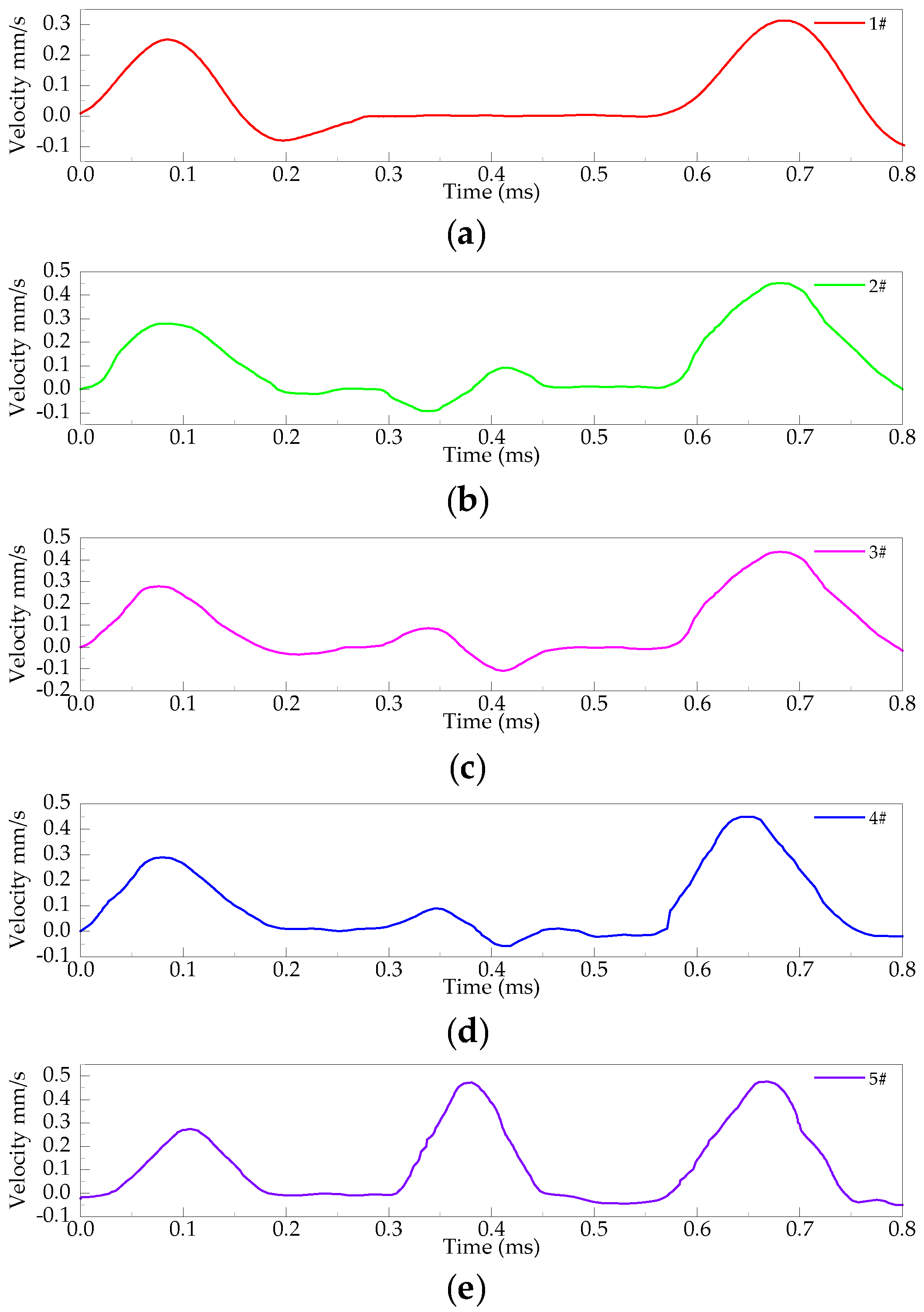
We define 1, 2, 3, 4, and 5 to mean intact pile, expanded diameter pile, reduced diameter pile, separated pile, and broken pile, respectively. g denotes layered soil, h denotes layered soil boundary in the upper part of the defect, and i layered soil boundary in the lower part of the defect. The labels for the classification categories are shown in

Table 9. Classification category labels.

Label	1	2	3	4	5	6	7	8	9
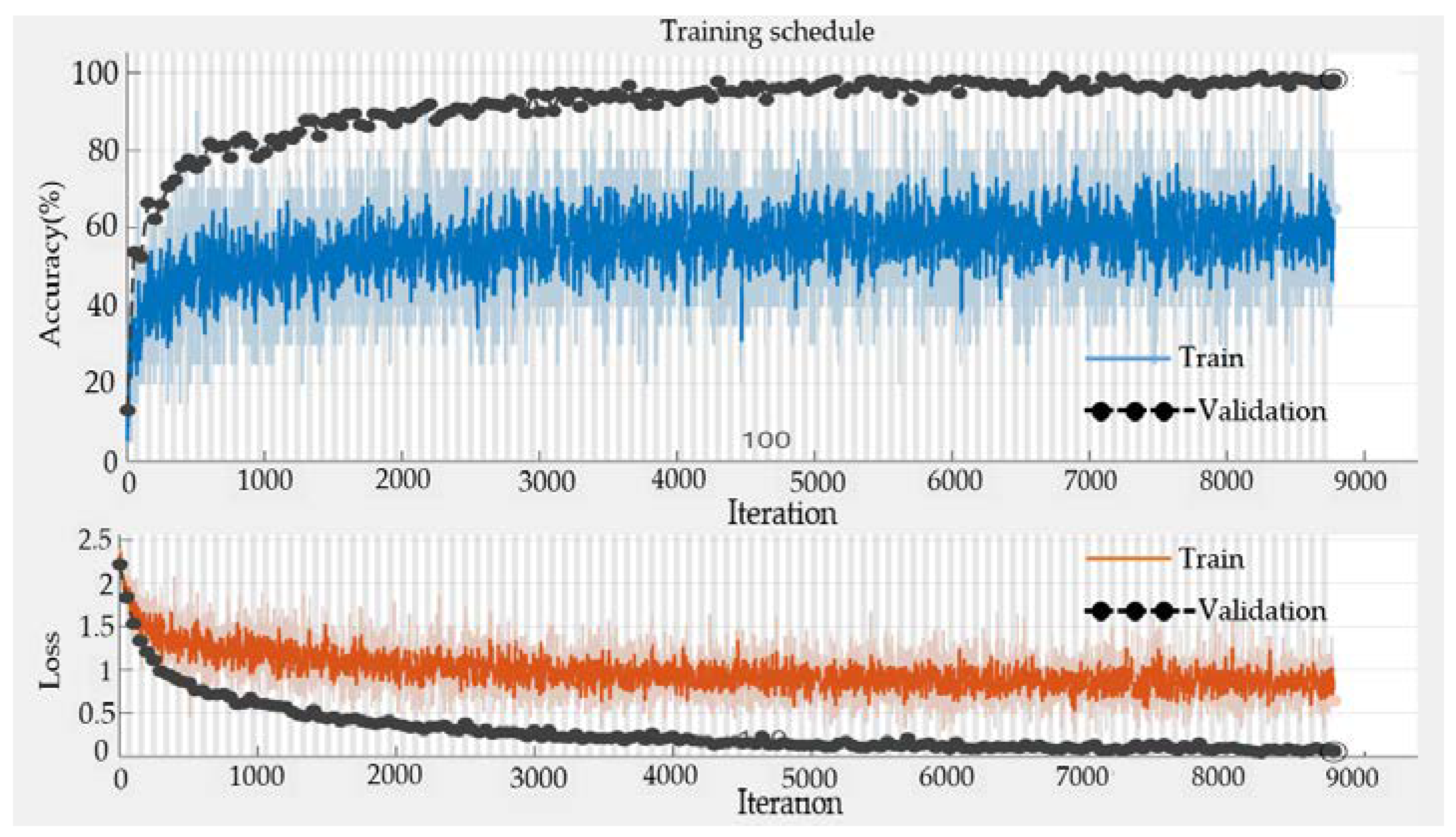
Scenarios	1-G	H-2	2-I	H-3	3-I	H-4	4-I	H-5	5-I

. After that, the CNN models were used to identify the categories. In Figure 14, the training schedule is displayed.

The training results of the CNN revealed that the accuracies of the training base were 98.67%, and the validation set was 98.33%.

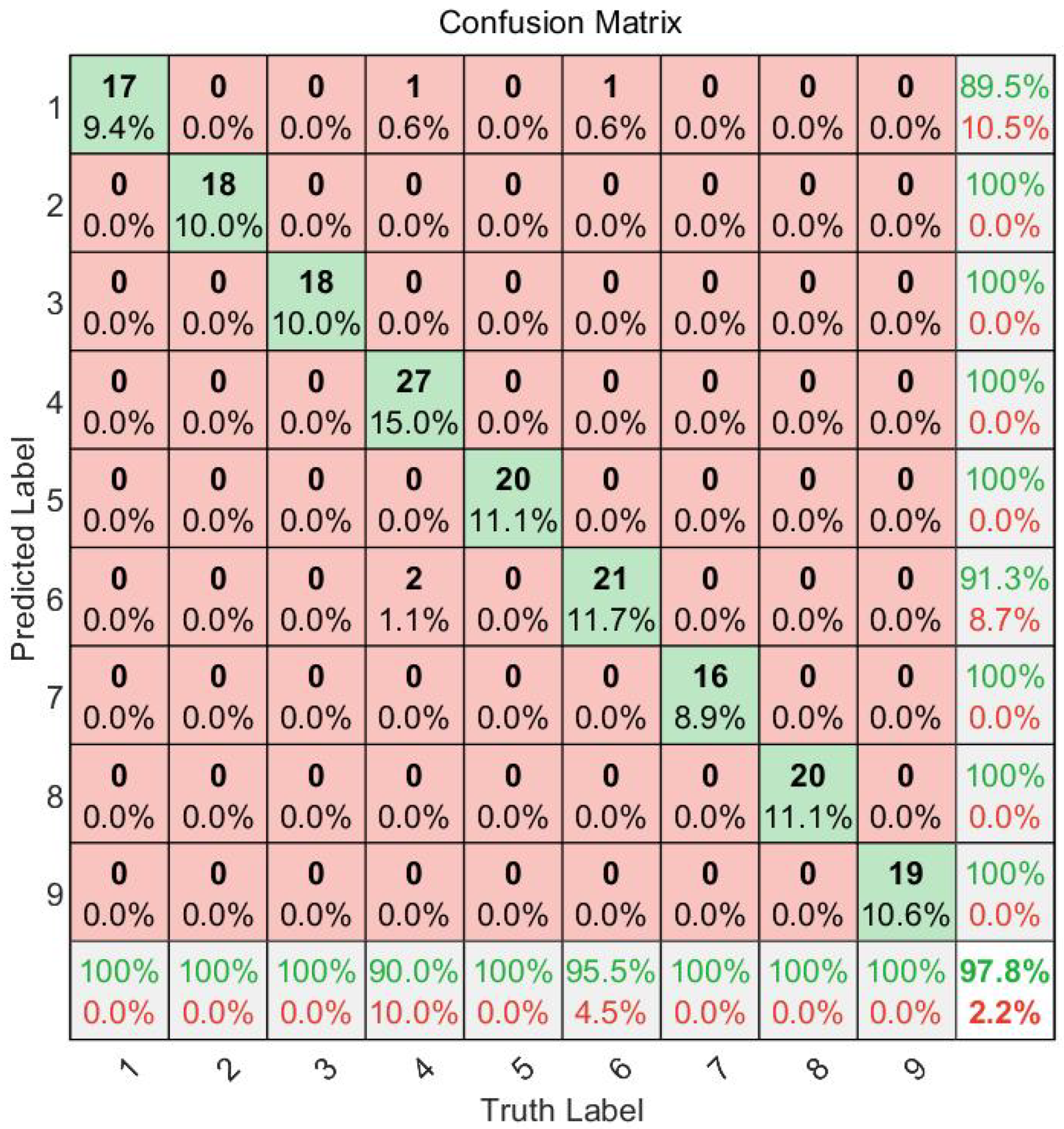
The CNN prediction findings in this research are presented using a mixed matrix. The pink box in the confusion matrix depicts the proportion of predictions that deviate from the actual values. The green diagonal line indicates that the expected results match the test labels. Figure 15 demonstrates that such a CNN recognition model has an accuracy rate of 97.8%, with lower identification rates of 90% and 95.5% for classes 4 and 6, respectively. The remaining categories all received 100% recognition. To avoid the impact of soil formation on the dynamic testing curve of layered soil, the model can accurately identify the type of faults and the location of layered soil.

3.2. CNN Recognition Results for Different Domain Features

This paper uses this classifier for comparative analysis from the perspective of feature composition, respectively, with the division of the sample dataset remaining unchanged, to further illustrate the accuracy of multi-domain features combined with CNN for recognizing foundation pile defects.

Table 10. Comparison of recognition results for different domain features.

CNN	Accuracy (%)
	Time Domain	Frequency Domain	Time–Frequency Domain	Multi-Domain
Train	89.00	81.89	88.56	98.67
Validation	87.50	80.28	86.67	98.33
Test	88.89	77.22	86.11	97.80

displays the accuracy results for CNN model recognition in the time, frequency, and time–frequency domains, respectively.

The analysis of Table 10 reveals that the test accuracy achieved by the suggested method is 97.78%, which is significantly higher than any single-domain characteristics. This suggests that multi-domain features offer more excellent feature information in CNN recognition than single-domain features.

3.3. Probabilistic Neural Network (PNN) Pile defect Identification

A feed-forward neural network constructed from radial basis function networks, the Probabilistic Neural Network classifier (PNN classifier), was used in an experiment comparison to demonstrate the superiority of the CNN model further. It is a supervised network classifier that uses Bayes classification rules and is based on the idea of probabilistic statistics. This study used the Parzen window function density estimation approach to estimate the conditional probability when performing classification pattern recognition. The Parzen method yields the probability density function estimation equation shown below.

$$f_A(X)=\frac{1}{{(2\pi )}^{p/2}{\delta }^p}\frac{1}{m}$$

(17)

$${\displaystyle \sum \exp \left[-\frac{{(X-X_{ai})}^T(X-X_{ai})}{2{\delta }^2}\right]}$$

(18)

In the formula, X_ai is the ith training vector of the defect pattern, m is the training sample quantity of the defective pattern, and the δ smoothing parameter.

The construction process of the PNN recognition model is as follows.

Step 1: We created a training set consisting of 9 × 120 data samples and a test set consisting of 9 × 140 data samples obtained from numerical simulations.

Step 2: Defective category is the intended result, and existing defective feature data is used as the input to the training samples. After training, a PNN model for defect classification and recognition is obtained from the network.

Step 3: Testing of the network’s performance was performed. Regression simulations were run on the training samples after the connection weights between the neurons in each layer were replaced in the network. The network was successfully trained and could be used to predict the class of unknown samples when the expected output of the training samples matched the simulated output of the PNN network.

Step 4: Classification prediction of unknown defective sample data using the constructed PNN model.

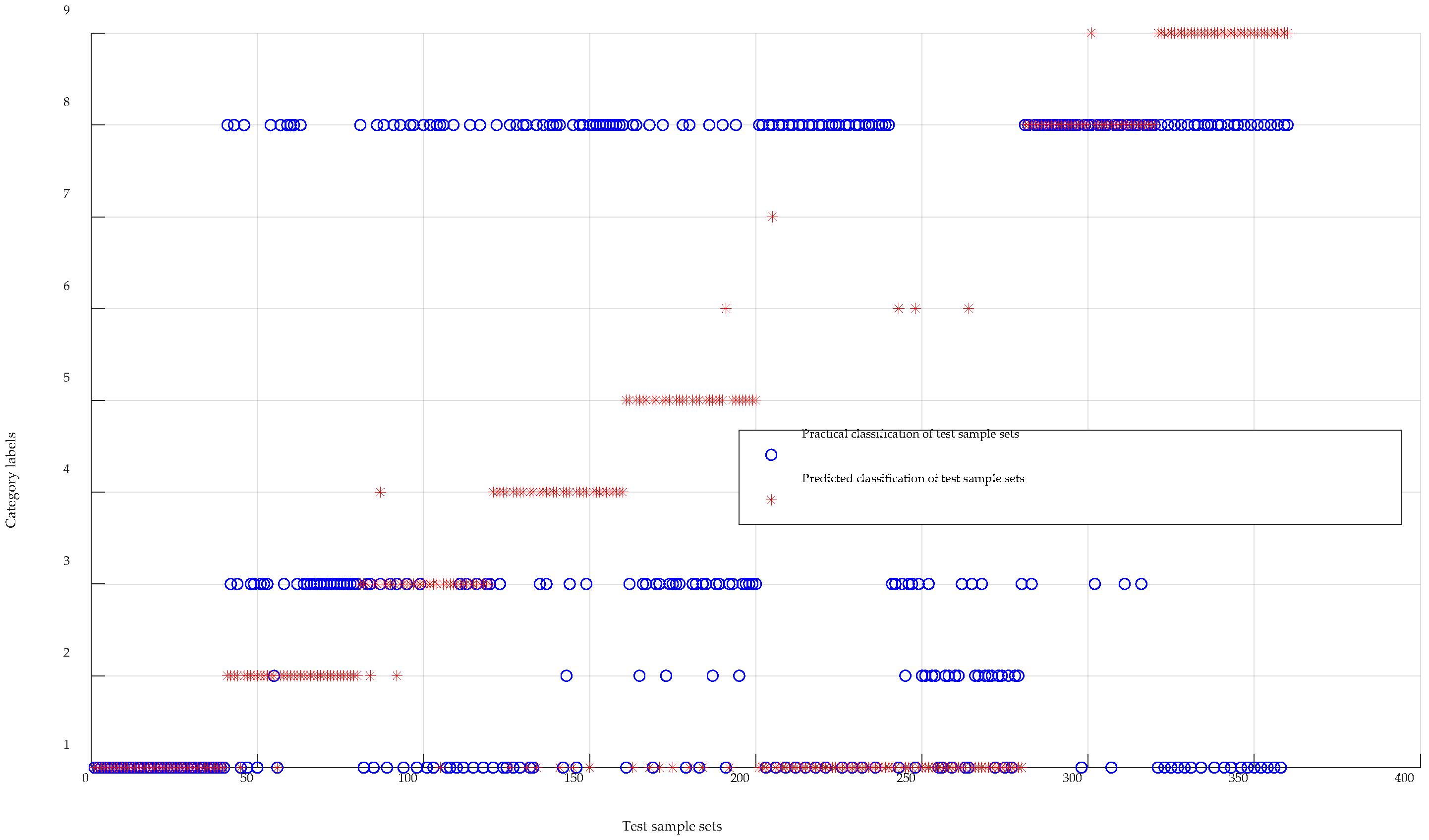
The category names used in this experiment adhere to the plan described in Section 3.1. Figure 16 displays the PNN classification findings, while

Table 11. PNN ‘s accuracy for different scenarios.

Scenarios	Number of Test Samples	Correct Recognition Number	Accuracy
1-G	40	60	45.5%
H-2	40	1	2.5%
2-I	40	9	25.0%
H-3	40	0	0
3-I	40	0	0%
H-4	40	0	0%
4-I	40	0	0%
H-5	40	33	84.6%
5-I	40	0	0%
Average accuracy 28.6%

displays the precise classification accuracies. In Figure 16, the symbols ○ and * stand for the actual and expected labels, respectively. When they overlap, the predicted labels match the actual ones. This model’s recognition accuracy was only 28.6%.

4. Conclusions and Future Work

To boost the effectiveness of pile recognition work, this research studies the reflected wave signal characteristics of foundation piles in layered soils using the traditional low-strain reflected wave method. In order to automatically classify and identify pile flaws, the signal is processed to extract feature indicators from three dimensions: time domain, frequency domain, and time–frequency domain. This is done in conjunction with a neural network. The following are the primary conclusions.

(1)

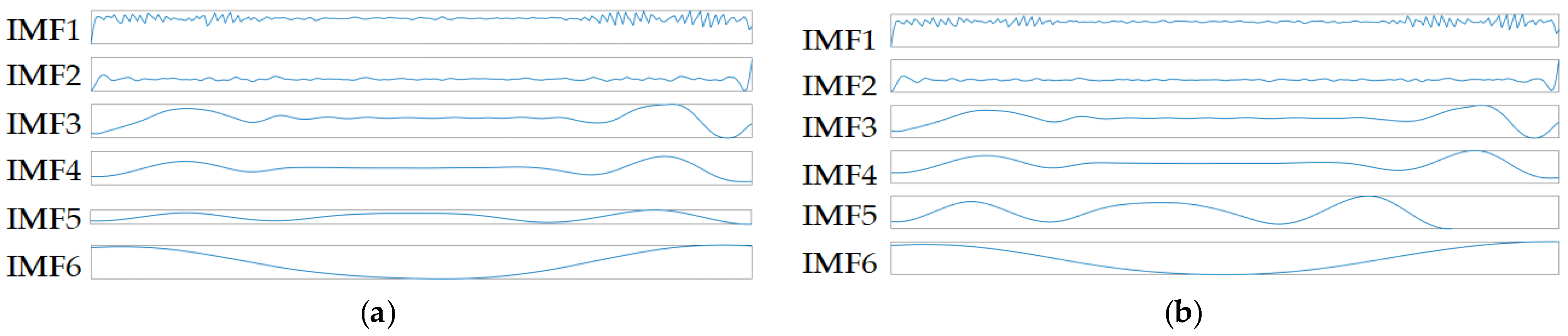
When the ICEEMDAN technique is utilized to decompose reflected wave signals from foundation piles under paved soil conditions, it lays the foundation for the accuracy of CNN identification. The correlation coefficient criterion filters the valuable components, removing the redundant components.

(2)

The convolutional neural network was used to classify and identify each group, and the feature sets extracted from the three dimensions were fed into the network with an accuracy of more than 90%, proving the excellent reliability of the CNN model for the detection of the foundation pile problem.

(3)

When single-domain features for foundation pile recognition were fed into the CNN model, the results were 88.89% for time domain features, 77.22% for frequency domain features, and 86.11% for time–frequency domain features. The accuracy of the multi-feature extraction method in conjunction with CNN is 97.8%. This method has high accuracy and effectively distinguishes the kind of foundation pile when the soil surrounding the pile is stratified, increasing the inspectors’ effectiveness.

Due to the irregular geometries of foundation pile flaws in real projects and the complexity of the geological environment, practical engineering necessitates more advanced detecting tools and data processing approaches. The accuracy of foundation pile identification utilizing the low-strain reflection wave method in layered soils may be significantly improved, and foundation pile flaws in layered soils can be automatically diagnosed in this study. These findings are significant for technical applications and have some theoretical importance. Although this paper’s pile defect identification model achieves good identification results based on supervised learning, the data sample cannot contain all the pile defect data in the project, and the pile defects are unknown. As a result, it is necessary to explore how to achieve high accuracy in the small sample and apply unsupervised learning algorithms in pile defects to improve the theoretical significance and practical value.

References

1. Cui, D.M.; Yan, W.Z. Towards intelligent interpretation of low strain pile integrity testing results using machine learning techniques. Sensors 2017, 17, 2443. [Google Scholar] [CrossRef]
2. Kim, H.J.; Mission, J.L.; Dinoy, P.R.; Kim, H.S.; Park, T.W. Guidelines for impact echo test signal interpretation based on wavelet packet transform for the detection of pile defects. Appl. Sci. 2020, 10, 2633. [Google Scholar] [CrossRef]
3. Dong-zi, P.A.N. Wavelet Analysis and Its Application in Integrity Testing of Piles; Institute of Rock & Soil Mechanics, The Chinese Academy of Sciences: Wuhan, China, 2003. [Google Scholar]
4. Ye, W. Integrity Testing of Piles Based on Finite Element Methods and Wavelet Transformations; Huazhong University of Science and Technology: Wuhan, China, 2005. [Google Scholar]
5. Tang, Y.D.; Feng, Y.Q. Wavelet analysis of dynamic testing signal of foundation pile. J. Vib. Shock. 2010, 29, 131–135. [Google Scholar]
6. Huang, N.E.; Shen, Z. The empirical mode decomposition and the hilbert spectrum for nonlinear and non-stationary time series analysis. Proc. R. Soc. Lond. 1988, 454, 903–995. [Google Scholar] [CrossRef]
7. Wu, Z.H.; Huang, N.E. Ensemble empirical mode decomposition: A noise-assisted data analysis method. Adv. Adapt. 2009, 1, 1–41. [Google Scholar] [CrossRef]
8. Torres, M.E. A complete ensemble empirical mode decomposition with adaptive noise. In Proceedings of the IEEE International Conference on Acoustics, Speech and Signal Processing (ICASSP), Prague, Czech Republic, 22–27 May 2011; pp. 4144–4147. [Google Scholar]
9. Colombians, M.A.; Schlotthauer, G.; Torres, M.E. Improved complete ensemble EMD: A suitable tool for biomedical signal processing. Biomed. Signal Process. Control. 2014, 14, 19–29. [Google Scholar]
10. Cai, Q.Y. Pile Defect Diagnosis Based on Wavelet Analysis and Neural Network; Huaqiao University: Quanzhou, China, 2002. [Google Scholar]
11. Bai, Q.L. Wavelet Transform on the Signal of Pile Integrity Testing; Huazhong University of Science and Technology: Wuhan, China, 2015. [Google Scholar]
12. Jiang, X.L. The Numerical Simulation and Experimental Research on Low-Strain Integrity Testing Are Based on Wavelet Analysis; South China University of Technology: Guangzhou, China, 2013. [Google Scholar]
13. Kang, W.X.; Li, J.D. The singularity detection of stress wave signal in one-dimensional components based on quantitative information entropy. Int. J. Signal Process. 2015, 10, 203–212. [Google Scholar]
14. Li, J.D. Feature Vector Extraction and Evaluation of Damage Information in One-Dimensional Component Based on the Stress Wave Signal; Harbin Institute of Technology: Harbin, China, 2016. [Google Scholar]
15. Kang, W.X. Research on Pile Foundation Defect Detection Technology Based on Wavelet and Support Vector Machine; Harbin Institute of Technology: Harbin, China, 2010. [Google Scholar]
16. Li, Z.B. Pile Foundation Defects Identification Based on Wavelet Analysis and Support Vector Machine; Changsha University of Science & Technology: Changsha, China, 2012. [Google Scholar]
17. Xue, Z.J.; Zhang, J.L. Pile defect severity recognition method based on wavelet packet analysis and support vector machine. Bridge Tunn. Eng. 2018, 167, 216–220. [Google Scholar]
18. Lin, H.; Yu, Y.Y. Analysis of pile defect detection based on wavelet analysis and neural network. Mod. Ind. Econ. Inf. 2016, 125, 84–85. [Google Scholar]
19. Zhao, Y.Y.; Yang, C.M. Prediction of foundation pile integrity based on RBF neural network. Constr. Technol. 2020, 49, 69–72. [Google Scholar]
20. Li, J.B. Numerical Simulation and Application Research of Bridge Foundation Pile Detection by Elastic Wave Method in Southern Sichuan Intercity Railway; Southwest Jiaotong University: Chengdu, China, 2020. [Google Scholar]
21. Guangdong Construction Engineering Quality and Safety Supervision and Inspection Station. Engineering Pile Quality Testing Technology Training Materials; China Building Industry Press: Beijing, China, 2009. [Google Scholar]
22. Fei, k.; Wei, Z.J. Application of ABAQUS in Geotechnical Engineering; China Water Conservancy and Hydropower Publishing House: Beijing, China, 2020; pp. 255–259. [Google Scholar]
23. Trochanis, A.M.; Bielak, J.; Christiano, E. Simplified model for analysis for one or two piles. J. Geotech. Eng. 1991, 3, 448–466. [Google Scholar] [CrossRef]
24. Zeng, Y.J.; Wang, N.X. Experimental study on centrifugal model of micropile foundation in soft soil area. Chin. J. Geotech. Eng. 2003, 2, 242–245. [Google Scholar]
25. Cooke, R.W.; Price, Q.; Tarr, K. Jacked piles in Londen clay: Interaction and ground behavior under working conditions. Geotechnique 1980, 2, 97–136. [Google Scholar] [CrossRef]
26. Li, H.B. Application and ABAQUS numerical simulation for the curves of dynamic pile testing based on entity model. Geotech. Investig. Surv. 2011, 9, 87–90. [Google Scholar]
27. Xu, H.L. The Response Characteristics of the Reflected Wave on Abnormal Piles and the Application Research of Simulation; Anhui University of Science and Technology: Huainan, China, 2017. [Google Scholar]
28. Lin, Y.Y.; Zhang, H.; Tang, L.Q. Research on low strain dynamic response of internal and external defects to piles in layered soil. Guangdong Archit. Civ. Eng. 2013, 12, 37–39. [Google Scholar]
29. Fu, Z.C. The Application of Numerical Simulation Technology in Low Strain Reflected Wave Method; Southwest Jiaotong University: Chengdu, China, 2011. [Google Scholar]
30. Wang, C.H.; Zhang, W. A neural network model for diagnosing pile integrity based on reflection wave method. Rock Soil Mech. 2003, 24, 952–956. [Google Scholar]
31. Liu, Z. ABAQUS 6.6 Basic Tutorials and Examples; China Water and Power Press: Beijing, China, 2008; pp. 129–130. [Google Scholar]
32. Zhuang, Z.; Zhang, F. ABAQUS Nonlinear Finite Element Analysis and Examples; Science Press: Beijing, China, 2005; pp. 52–93. [Google Scholar]
33. Chen, F.; Xu, T.P. Pile Quality Detection Technology; China Building Industry Press: Beijing, China, 2014; pp. 104–110. [Google Scholar]
34. Zhong, L.D. Application of low strain reflection wave method in construction quality testing of pile foundation. Railw. Stand. Des. 2012, 04, 35–37. [Google Scholar]
35. Li, Y.B.; Huang, D.H. Gear fault diagnosis method based on deep belief network and information fusion. J. Vib. Shock. 2021, 40, 62–69. [Google Scholar]
36. Peng, Z.M.; Cheng, L.S. Research on rolling bearing fault classification method based on multi-feature extraction and improved Matian system. J. Vib. Shock. 2020, 39, 249–256. [Google Scholar]
37. Xie, Y.F.; Fu, Y. Bearing fault diagnosis based on multi-feature extraction and LSSVM. Mach. Tool Hydraul. 2020, 48, 188–190. [Google Scholar]
38. Zhang, B.; Zhang, S.; Li, W. Bearing performance degradation assessment using long short-term memory recurrent network. Comput. Ind. 2019, 106, 14–29. [Google Scholar] [CrossRef]
39. Xu, X.; Han, H.M. Fault identification of key components of diesel engine based on multi-feature extraction and KECA. Electron. Meas. Technol. 2021, 44, 63–68. [Google Scholar]
40. Wan, X.L.; Gao, E.G. Frequency domain analysis method in pile integrity detection. Coal Geol. China 2000, 12, 67–68. [Google Scholar]
41. Liu, Q. Research on Fault Diagnosis and Remaining Life Prediction of Rolling Bearings Based on Convolutional Neural Network; Jilin University: Changchun, China, 2021. [Google Scholar]
42. Liu, L.L.; Zhu, J. Non-destructive detection of anchor defects using ultrasonic guided wave and ICEEMDAN method. Earth Sci. 2022, 66, 1–17. [Google Scholar]
43. Xing, S.L. Hilbert-Huang transfer analysis on vehicle-induced vibration signal of continuous bridges based on ICEEMDAN. J. Southwest Jiaotong Univ. 2021, 56, 476–492. [Google Scholar]
44. Wang, H.N.; Cui, B.Z. Fault diagnosis of planetary gearbox using ICEEMDAN and SVM. Mech. Sci. Technol. Aerosp. Eng. 2022, 42, 1–7. [Google Scholar]
45. Liu, M.D. Research on Damage Identification Of Truss Based on Acceleration Signal; Lanzhou Jiaotong University: Lanzhou, China, 2020. [Google Scholar]
46. Fang, Y.L. Damage identification of frame structure based on wavelet packet sample entropy and support vector machine. Sci. Technol. Eng. 2021, 21, 5862–5869. [Google Scholar]
47. Sarmadi, H.; Entezami, A. Application of supervised learning to validation of damage detection. Arch. Appl. Mech. 2021, 91, 393–410. [Google Scholar] [CrossRef]
48. Angulo-Saucedo, G.A.; Leon-Medina, J.X.; Pineda-Muñoz, W.A.; Torres-Arredondo, M.A.; Tibaduiza, D.A. Damage classification using supervised self-organizing maps in structural health monitoring. Sensors 2022, 22, 1484. [Google Scholar] [CrossRef]
49. Sun, Y.; Ma, S.; Sun, S. Partial discharge pattern recognition of transformers based on mobilenets convolutional neural network. Appl. Sci. 2021, 11, 6984. [Google Scholar] [CrossRef]
50. Nair, V.; Hinton, G.E. Rectified linear units improve restricted boltzmann machines. In Proceedings of the ICML, Haifa, Israel, 21–24 June 2010. [Google Scholar]
51. Liu, W.P.; Tian, S.W. Classification of pile integrity using convolutional neural network. J. Nanchang Univ. 2021, 43, 263–268. [Google Scholar]
Figure 1. Pile–soil model.
Applsci 12 09840 g001
Figure 2. The curve of unit hammer load versus time.
Applsci 12 09840 g002
Figure 3. Mesh division of pile–soil model.
Applsci 12 09840 g003
Figure 4. Model piles.
Applsci 12 09840 g004
Figure 5. Model dynamic test results: (a) 1# model pile; (b) 2# model pile; (c) 3# model pile; (d) 4# model pile; (e) 5# model pile.
Applsci 12 09840 g005
Figure 6. Dynamic signal analysis system and components.
Applsci 12 09840 g006
Figure 7. Pile models: (a) 1# complete pile, 2# diameter expanding pile, 3# diameter shrinkage pile, 4# segregation pile, and 5# broken pile; (b) Placement of model pile.
Applsci 12 09840 g007
Figure 8. Pile integrity testing field.
Applsci 12 09840 g008
Figure 9. Comparison of finite element simulation results and experimental results: (a) 1# model pile; (b) 2# model pile; (c) 3# model pile; (d) 4# model pile; (e) 5# model pile.
Applsci 12 09840 g009
Figure 10. ICEEMDAN decomposition of reflective wave signal of complete pile: (a) Soil boundary position near pile tip; (b) Soil boundary position near pile base.
Applsci 12 09840 g010
Figure 11. Correlation analysis variation tendency: (a) Complete pile dynamic signal ICEEMDAN decomposition; (b) Diameter expanding piles dynamic signal ICEEMDAN decomposition; (c) Diameter shrinkage piles dynamic signal ICEEMDAN decomposition; (d) Segregation pile dynamic signal ICEEMDAN decomposition; (e) Pile breaking dynamic signal ICEEMDAN decomposition.
Applsci 12 09840 g011
Figure 12. CNN model.
Applsci 12 09840 g012
Figure 13. Recognition model.
Applsci 12 09840 g013
Figure 14. CNN model training schedule.
Applsci 12 09840 g014
Figure 15. CNN model classification prediction results.
Applsci 12 09840 g015
Figure 16. PNN model classification prediction results.
Applsci 12 09840 g016