Article

Forecast of Airblast Vibrations Induced by Blasting Using Support Vector Regression Optimized by the Grasshopper Optimization (SVR-GO) Technique

by
Lihua Chen
1,
Panagiotis G. Asteris
2,*,
Markos Z. Tsoukalas
2,
Danial Jahed Armaghani
3,
Dmitrii Vladimirovich Ulrikh
3 and
Mojtaba Yari
4
1
Department of Civil Engineering, Chongqing Vocational Institute of Engineering, Jiangjin District, Chongqing 402260, China
2
Computational Mechanics Laboratory, School of Pedagogical and Technological Equation, 15122 Maroussi, Greece
3
Department of Urban Planning, Engineering Networks and Systems, Institute of Architecture and Construction, South Ural State University, 76, Lenin Prospect, 454080 Chelyabinsk, Russia
4
Department of Mining Engineering, Faculty of Engineering, Malayer University, Malayer 65719-95863, Iran
*
Author to whom correspondence should be addressed.
Appl. Sci. 2022, 12(19), 9805; https://doi.org/10.3390/app12199805
Submission received: 23 August 2022 / Revised: 10 September 2022 / Accepted: 13 September 2022 / Published: 29 September 2022
(This article belongs to the Special Issue Blast and Impact Engineering on Structures and Materials)

Abstract

:
Air overpressure (AOp) is an undesirable environmental effect of blasting. To date, a variety of empirical equations have been developed to forecast this phenomenon and prevent its negative impacts with accuracy. However, the accuracy of these methods is not sufficient. In addition, they are resource-consuming. This study employed support vector regression (SVR) optimized with the grasshopper optimizer (GO) algorithm to forecast AOp resulting from blasting. Additionally, a novel input selection technique, the Boruta algorithm (BFS), was applied. A new algorithm, the SVR-GA-BFS7, was developed by combining the models mentioned above. The findings showed that the SVR-GO-BFS7 model was the best technique (R2 = 0.983, RMSE = 1.332). The superiority of this model means that using the seven most important inputs was enough to forecast the AOp in the present investigation. Furthermore, the performance of SVR-GO-BFS7 was compared with various machine learning techniques, and the model outperformed the base models. The GO was compared with some other optimization techniques, and the superiority of this algorithm over the others was confirmed. Therefore, the suggested method presents a framework for accurate AOp prediction that supports the resource-saving forecasting methods.

1. Introduction

Air-overpressure (AOp) or airblast is an unwelcome outcome of blasting in mining operations. The blasting creates temporary air blast pressure waves that persist for some time [1,2]. More than 20% of the explosive energy is used to fracture and replace the rock fragments. More than 70% of this energy is dissipated, which causes AOp and other unwanted phenomena [1]. Various parameters, including terrain circumstances, blast design, and climate, are influential on AOp [2,3]. The enormous shock waves coming out of the blast spot toward the free facade create AOp. Hence, the AOp can be defined as a shock wave deflected laterally by density changes in the air. These AOp waves are released with some audible high- or low-frequency sounds. AOp can cause structural damage and harm to people in the vicinity of quarry sites [4].
Several studies attempted to establish associations for the AOp forecast using its influential factors. Kuzu et al. [5] ascertained an experimental association between AOp and interval among blast planes and monitoring spot and mass of explosive substances (32%). To reproduce ground shock and air explosion tensions deriving from facade explosions, Wu and Hao [6] connected Autodyn2D to mathematical models, wherein properties of rock materials and free air were involved. A partial-empirical model for forecasting the airwave tension caused by blasting operations outside a tunnel was developed by Rodríguez et al. [7]. They claim that their model works in different situations. Rodríguez et al. [8] proposed a photometric curve and iso-attenuation curves to describe the phenomenon, as well as a proposed charge-distance curve to resolve the query.
Recently, various investigations have applied machine learning (ML) techniques to resolve science and engineering problems [9,10,11,12,13,14,15,16,17,18,19]. Such techniques were used to predict the AOp values and identify the most influential predictors [20,21,22]. These techniques are both time and cost-saving and can help both researchers and practitioners allocate resources to other necessary operations. Among the ML algorithms, artificial neural networks (ANNs) and an adaptive neuro-fuzzy inference system (ANFIS) were employed more frequently than other techniques in the investigations of AOp [23]. Some studies used tree-based techniques such as XGBoost, random forest (RF), and M5 [24]. Rare studies employed support vector regression to predict the AOp [25]. Additionally, some of these models were optimized with some techniques to improve accuracy and efficiency. Some of these optimization techniques include genetic algorithms (GA) and particle swarm optimization (PSO) [2]. Lastly, different methods, such as fuzzy Delphi methods, were used to choose the inputs before the model was built [26].
Despite the vast application of ML algorithms for AOp prediction, various efficient models for prediction, optimization, and input selection are neglected. In this study, the authors developed a novel prediction model that encompasses SVR as a prediction model, the Grasshopper algorithm for optimizing the SVR’s hyperparameters, and the Boruta algorithm (BFS) for input selection. The Grasshopper algorithm is used in this study because it is easy to use, has a structure without gradients, avoids local optimums well, and treats problems as black boxes. SVR is rarely employed for AOp prediction, and to the best of the authors’ knowledge, the Grasshopper and Boruta algorithms have not been applied in this domain. The rest of this paper is structured as follows: the next section discusses algorithms used in this study, including SVR, GO, and BFS. Additionally, the case study of this research will be explained in this section. The results and discussions’ section describes the data preparations and performance criteria. The results of input selection and model optimization are reported in this section. The paper ends with a conclusion that sums up what was learned from this study and makes some suggestions for future research.

2. Material and Methods

This section thoroughly describes the methods used in this study. These methods include SVR as a well-known prediction technique, GO as a metaheuristic optimization technique and BFS as an input selection approach. The SVR-GO-BFSn model, which is the result of combining the algorithms mentioned above, is adequately explained. Furthermore, four ML techniques and three optimization techniques were applied to verify the performance of the SVR-GO-BFSn model.

2.1. Data Collection

Data for this study was collected from a published work by Hajihassani et al. [27]. According to their study, four granite mines were selected and considered for data collection in the Johor area, Malaysia. In total, 62 blasting operations were performed. The main substance of the explosion was ANFO, a widely used bulk industrial explosive, the stemming substance was granular gravel, and the diameters of the blast holes were 75, 89, and 115 mm. The specifications of rock quality designation (RQD) as well as the height of the bench are shown in Table 1. Various blasting parameters, including RQD, burden, hole depth, spacing, powder factor, and stemming length, were evaluated during the data collection.
The research team observed the AOp employing microphones (L type), which were linked to the AOp grooves of record-keeping elements. The AOp values ranged from 88 dB to 148 dB. To ensure an accurate measurement of overpressures, the operating frequency response of microphones was selected between 2 and 250 Hz. This frequency is suitable for measuring the overpressure for both human hearing and construction.
The minimum values of 10 m, 0.34 kg/m3, 60 kg, 1.7 m, 1.5 m, 2.65 m, 60%, 12, 300 m, and 89.1 dB were recorded for hole depth, powder factor, maximum charge per delay, stemming, burden, spacing, RQD, no. of hole, distance from the blast face, and AOp, respectively, while the values of 25 m, 0.76 kg/m3, 171 kg, 3.2 m, 4 m, 91%, 63, 600 m, and 126.3 dB were recorded as maximum amounts of the same variables. More information regarding the data used in this study can be found in the original study [27].

2.2. Preparation of Data

The min/max transformation technique was used to normalize the collected data. The objective of this transformation was to restrict the inputs’ possible advantages to those with noticeable numerical values, over those with small values. Handling large-value inputs can be challenging and complicated due to the fact that the kernel quantity relies on vectors’ internal multiplication of inputs. Therefore, conquering mathematical complications throughout calculation procedures is another crucial aspect of input normalization. The data were transformed using Equation (1) and the normalized data ranged from zero to one.
a i n = a i a m i n a m a x a m i n
where the input vectors with the calculated observation points are denoted by ai. amin and amax refer to the lowest and highest values that relate to the calculated data set. a i n is the transformed variant of ai.

2.3. Support Vector Regression (SVR)

One of the most effective approaches for handling regression complications is SVM, which is a supervised technique [28]. The formation and optimization approach of SVM varies according to the nature of inputs, and ε-SVR is the regression form of SVM. The principal objective of SVR is to acquire a hypothesis whose entire errors of regression forecast are situated within a predetermined threshold, ε. The next aim of the learned function is that this function possesses an excellent achievable generalization capability. This aim is purposely attempted in order that a flat model can be established. The following equations enact the aforementioned aims, forming a typical convex quadratic optimization problem with linear constraints set. The above goals are met by the following equations, which, along with the set of linear constraints, make a typical curved quadratic optimization problem.
m i n i m z e   1 2 ω 2 + c i = 1 k ( ϑ i + ϑ i * )
s u b j e c t   t o { b i ω , a i + c ϑ i + ε ,   n ω , a i + c b i   ϑ i * + ε , n   ϑ i ,   ϑ i * 0 , n  
where, for training points (ai, bi), ..., (an, bn), k denotes the number of data samples, the vectors of ai denote values of input, and bi implies the corresponding output value for ai. The upper and lower errors of training are represented by ϑ i and ϑ i * , respectively. The errors are indifferent to a particular margin defined by ε; afterwards, the cost function will be added by penalties. The normal vector is denoted by ω . The regularization parameter (c > 0) regulates the balance of the pair of goals enacted in the above equations. The authors employed Lagrange multipliers to ascertain the SVR’s optimization problem expressed by the above equations. Some alterations were performed following that the Lagrangian is calculated until the next equation is obtained:
f ( a , β i , β i * ) = i = 1 n ( β i β i * ) l ( a , a i ) c
The equation obtained above is based on theories of optimality constraints, the kernel method, and Lagrange multipliers. While four renowned kernels, including sigmoid, polynomial, linear, and RBF, are available, this study employed RBF. This kernel was intentionally picked due to its computational capability. Typically, this kernel outperforms others [28]. RBF is extremely nonlinear, including possessing some inputs and an unlimited-dimensional space of mapping [29]. The RBF kernel is displayed in the following equation:
L ( a i , a j ) = e γ ( a i a j 2 )
where γ ∈ R, γ > 0 describes the expanse of the radial basis kernel function.
Figure 1 displays the structure of SVR based on Equation (3). This structure admits the requirements of Karush–Kuhn–Tucker for resolving a quadratic optimization query. The values of (βi–βi) were used to obtain the decision function. It is worth mentioning that these values were non-null support vectors. One of the most vital steps to develop a profoundly accurate and stable prediction model is to optimize the pair of SVR’s hyperparameters, including C and γ . Adopting optimization methods for ascertaining these parameters’ optimal conditions is considered in recent studies.

2.4. Grasshopper Optimization Algorithm (GO)

A recent swarm intelligence method, which is acknowledged as the grasshopper optimization (GO) algorithm, was employed in this study. Roles of nature are behind this method. This optimization technique was initially developed to deal with complicated optimization queries [29]. GO mimics the behavior of grasshopper colonies for resolving the queries of optimization. The GO involves two search processes: exploitation and exploration. Nymph and adult grasshoppers execute the search procedure. Typically, long intervals are covered by adult grasshoppers. Hence, they can search a whole space (global) to discover more suitable areas, where more foods are provided. In fact, the exploration procedure is performed by them. On the other hand, nymph grasshoppers perform the exploitation task, which means that they aim for a specific or local region. The GO secures an equilibrium between exploitation and exploration. This balance may lead to a slightly more complex algorithm. Mathematically, Saremi et al. [30] achieved a method to represent the colony function of grasshoppers. The following formula shows the mathematical model of the grasshoppers’ swarming function.
Y i = A i + B i + C i
where Yi denotes the ith grasshopper’s place. Ai indicates the idea of social interplay. So long as Bi expresses the strength of gravity forced on the ith grasshopper, the wind advection is demonstrated by Ci. Remarking that the formula was re-written Y i = m 1 A i + m 2 B i + m 3 C i to produce arbitrary behaviour, wherein m1, m2, and m3 are accidentally picked figures between zero and one. The three steps of the implementation of GO algorithm are shown in Table 2.
In the first step, the concepts of social interaction (Ai) and social forces (a(m)) were determined. The function “a” is able to divide the space amongst two grasshoppers into 3 areas: attraction, repulsion, and comfort. In the second step, the force of gravity imposed on the ith grasshopper was determined (Bi).
The wind advection (Ci) was established in the third step. It is worth mentioning that because the nymph grasshoppers do not have wings, the wind direction strongly impacts their movement. The elements of Ai, Bi, and Ci were replaced in Equations (6) and (11) was formed. Typically, the grasshoppers reach their pleasure areas rapidly, and the group does not gather in particular spots. Thus, Equation (11) is unable to deal with the optimization queries immediately. This equation was amended to solve the optimization issue mentioned above, and Equation (12) was created. As shown in Equation (12), “c” is a lessening coefficient which is utilized on the way to decrease the comfort, attraction, and repulsion areas. In this Equation, the “c” enters double because of the following reasons:
  • By expanding the abundance of iterations, the motion of marked grasshoppers is decreased by the initial “c”. This parameter equilibrates the whole exploration and exploitation of the target.
  • The following “c” decreases the repulsion, attraction, and comfort areas amongst grasshoppers. The aforementioned decline is proportionate to the iterations’ abundance.
GO needs to be avoided by becoming stuck in the local optimum. Alternatively, it attempts to acquire a precise calculation of the global optima. Grasshoppers achieve progressive equilibrium between exploration and exploitation because of the diverse pleasure area parameter “c”. In each iteration, the “c” can be calculated by Equation (13). In this study, the authors employed great rates of repulsion since this is a crucial method in the GO to circumvent local solutions. The outcomes reveal that great repulsion rates limit grasshoppers to staying at a local optimum. To summarize, Algorithm 1 depicts the processes involved in executing the GO.
Algorithm 1 GO optimization
1: Initialize the swarm population (grasshoppers) Yi, where i = (1, 2, …, N)
2: Initialize the parameters: cmin, cmax, D
3: Calculate the fitness value of each search agent
4: Assign O to the best search agent (the individual with highest fitness value)
5: while d < D do
6:   Use Equation (13) to update c
7:   for each search agent
8:     Normalize the distance between grasshoppers within [1,4]
9:     Update the position of the current search agent by Equation (12)
10:     Bring the current search engine back when it exceeds the boundaries
11:    end for
12:    if there is a better solution, update O
13:    d = d + 1
14: end while
15: Return O

2.5. Boruta Feature Selection (BFS) Algorithm

The BFS is an ensemble-based input selection technique that follows the function system of RF with some extra tools to obtain better outcomes [31]. The BFS attempts to identify all the important inputs in both regression and classification queries. The principal concept of this technique is employing analytical measurements and executing various RFs to examine the significance of the original inputs and inputs with an expanded randomness degree. The additional randomness allows a greater understanding of what inputs are significant. Figure 2 shows the running steps of BFS.
The BFS determines all important inputs in the knowledge system and renders the inputs’ importance degree. This system also designates significant inputs with numerical rates indicating their significance. Therefore, this may assist scholars in building various input mixtures based on their relevance ranking to determine the optimal input collection. Detailed information about the Boruta input selection technique can be obtained from Kursa and Rudnicki [31].

2.6. SVR-GO-BFSn Model Development

A hybrid model expressed by SVR-GO-BFSn was developed to improve the performance of the AOp forecast. The effective algorithms are combined into SVR-GO-BFSn: SVR, GO for optimizing parameters, and BFS for input choice. The parameterization of the SVR-GO-BFSn model was based on “n”, which showed the abundance of inputs engaging in developing the model in line with the “n” greatest importance values assigned by BFS. The most important inputs were selected using BFS. Next, GO was utilized to train SVR and optimize a pair of its hyperparameters (γ and C). Finally, the developed model was used to predict the AOp values. Figure 3 shows a fundamental flowchart of the model developed, which includes the main four steps.
Step one involved the preparation of data. The dataset included nine candidate inputs. In this step, the data were also normalized as previously described. The second step involved the selection of inputs using the BFS technique. This method contributed to a fair and logical determination and ranking of significant and insignificant inputs from the AOp dataset. In line with the significant input ranking, various input mixtures were built and expressed as n = 1, n = 2, …, n = all. If the “n” is one, it means that the input collection simply includes one input (the most significant input). If the “n” is two, it refers to an input set that involves the two most significant ones. If “n” equals “all”, it means that an input assortment involves all significant ones. Obtaining the minimum optimal input’s collection was the main objective of this method.
Step three engaged in the optimization of SVR utilizing GO. A pair of SVR’s parameters, including C and γ, were optimized by applying GO. Ultimately, various regression models (SVR-GO-BFSn) were developed based on various input mixtures.
Step four involved performing predictions using SVR-GO-BFSn. Utilizing the testing set, the corresponding built predictive models were assessed, and the forecast outcomes were reported. The most suitable model was picked following its precision and error performance. Therefore, the most suitable input set was regarded as the optimal collection of inputs and its C and γ were the optimal SVR values.

2.7. Validation Scheme

The training data employ a different pre-process once the AOp dataset has been randomly partitioned into the training (80%) and test (20%) sets. We call this method the k-fold cross-validation approach. This technique improves the models’ flexibility and, consequently, their precision. Therefore, the statistical examination would generalize properly to a particular dataset. In comparison with holdout validation, cross-validation is more suitable for datasets with a small sample size. This method randomly divides the initial data into k equivalent sub-data sets. Following that, the k-1 sub-data are used for training, and one sub-data set is used for testing the model. This procedure is repeated k times. Finally, a single approximation is achieved by averaging the k results from the folds. In this study, the k value is 10 (Figure 4).

3. Results and Discussion

3.1. Performance Criteria

Various performance criteria were utilized to gauge the performance of the models established in the present study. These metrics included squared correlation (R2), root mean square error (RMSE), mean absolute error (MAE) and mean absolute percentage error (MAPE). The formulations of these criteria are presented by Equations (14)–(17). These performance indices have been used by some other researchers as well in predictive and classification studies [32,33,34,35,36,37].
R 2 = 1 h = 1 N ( z i b ¯ ) 2 h = 1 N ( b i b ¯ ) 2
R M S E = 1 N h = 1 N ( z h b h ) 2
M A E = 1 N h = 1 N | z h b h |
M A P E = 1 N h = 1 N | z h b h b h | × 100 %
where N is the total quantity of samples; zh and bh signify predicted and real values; b ¯ is the mean value of b.

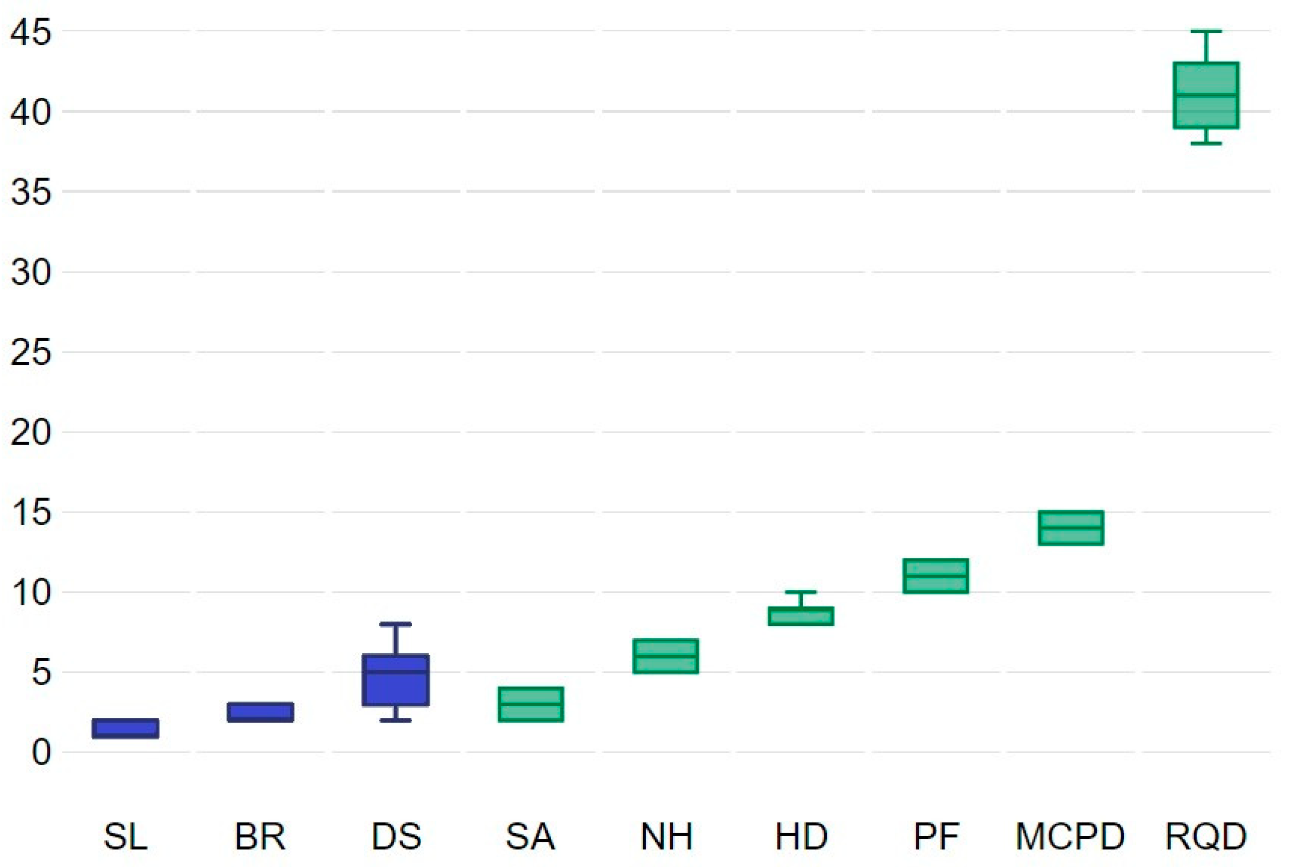
3.2. Input Selection

The BFS was applied to evaluate the significance of inputs for predicting the AOp. In the beginning, the suggested approach examined nine inputs for the final selection of the inputs, and 100 iterations were used to execute the BFS. The authors did not notice any variations in the research results exceeding 100 runs. The findings of the BFS-based technique are presented in Figure 5.
Box plots in 
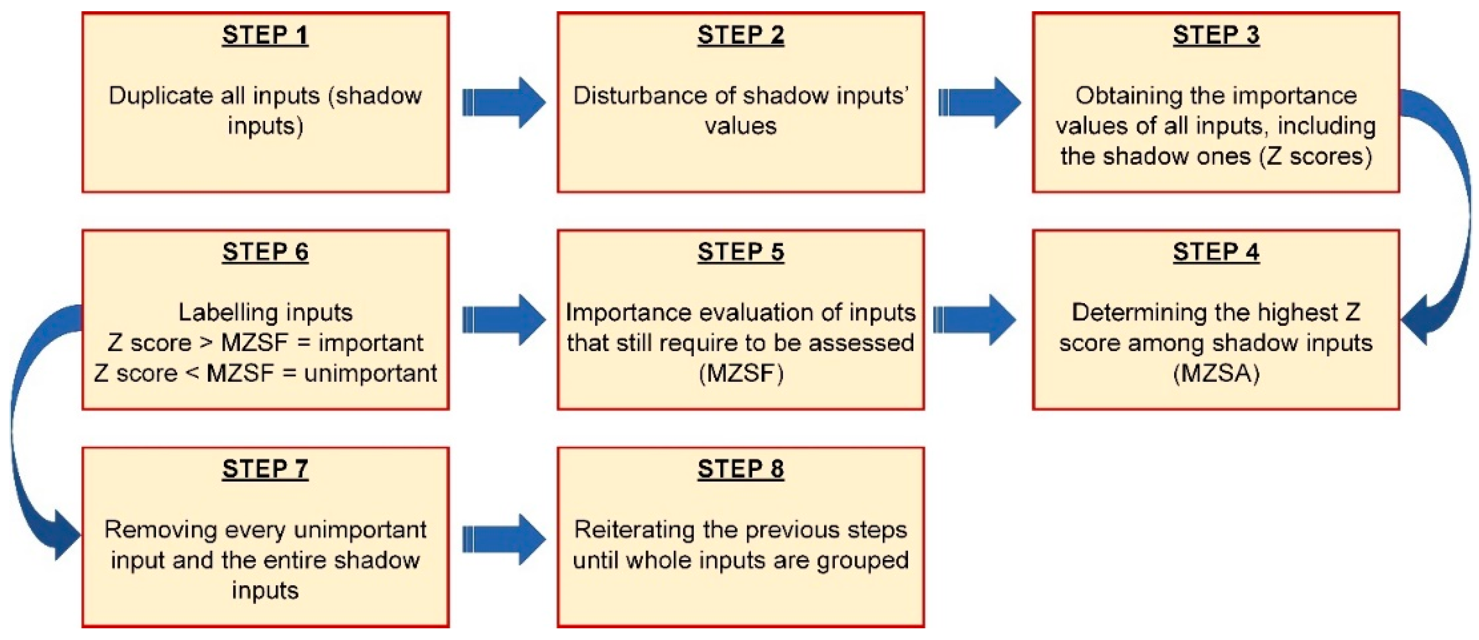
Figure 5 explain the significance of the inputs assessed through BFS. The green plots show those inputs that have more prominent predictability than those indicated by the blue colors. All inputs were classified as significant. Therefore, in developing various input mixtures for the AOp forecast, all nine inputs will be employed. Based on the suggested structure, nine predictive models will be proposed. This approach aims to determine the minimal optimal variable’s collection for overcoming the issues of underfitting and overfitting. Furthermore, the inputs indicated in red in the BFS results possess smaller informational potential compared with shadow traits. Hence, these inputs are eliminated from the final collection. Moreover, the yellow inputs show tentative ones. As a result, no inputs appeared tentative or unimportant.
The RQD, MCPD, and PF inputs were confirmed to be the most significant inputs, graded in the same descending form of value for the data obtained from the site. Following these inputs, the HD placed fourth in significance. These findings confirm that using the three characteristics of blasting improves the effectiveness of AOp predictability. Therefore, this study suggests that prospective scholars use these variables as inputs in their models. This algorithm is strong and can produce an unbiased and firm choice of significant and insignificant inputs from a dataset. Since combining more inputs can induce overfitting issues, the novel BFS’s capacity to prioritize inputs in decreasing sequence of values can assist scholars in deciding which inputs apply to the AOp forecast. Hence, dropping unnecessary or less correlated inputs may reduce calculation complications and time linked with enhancing the suggested hyperparameters of the scheme.

3.3. SVR-GO-BFSn Model Performance

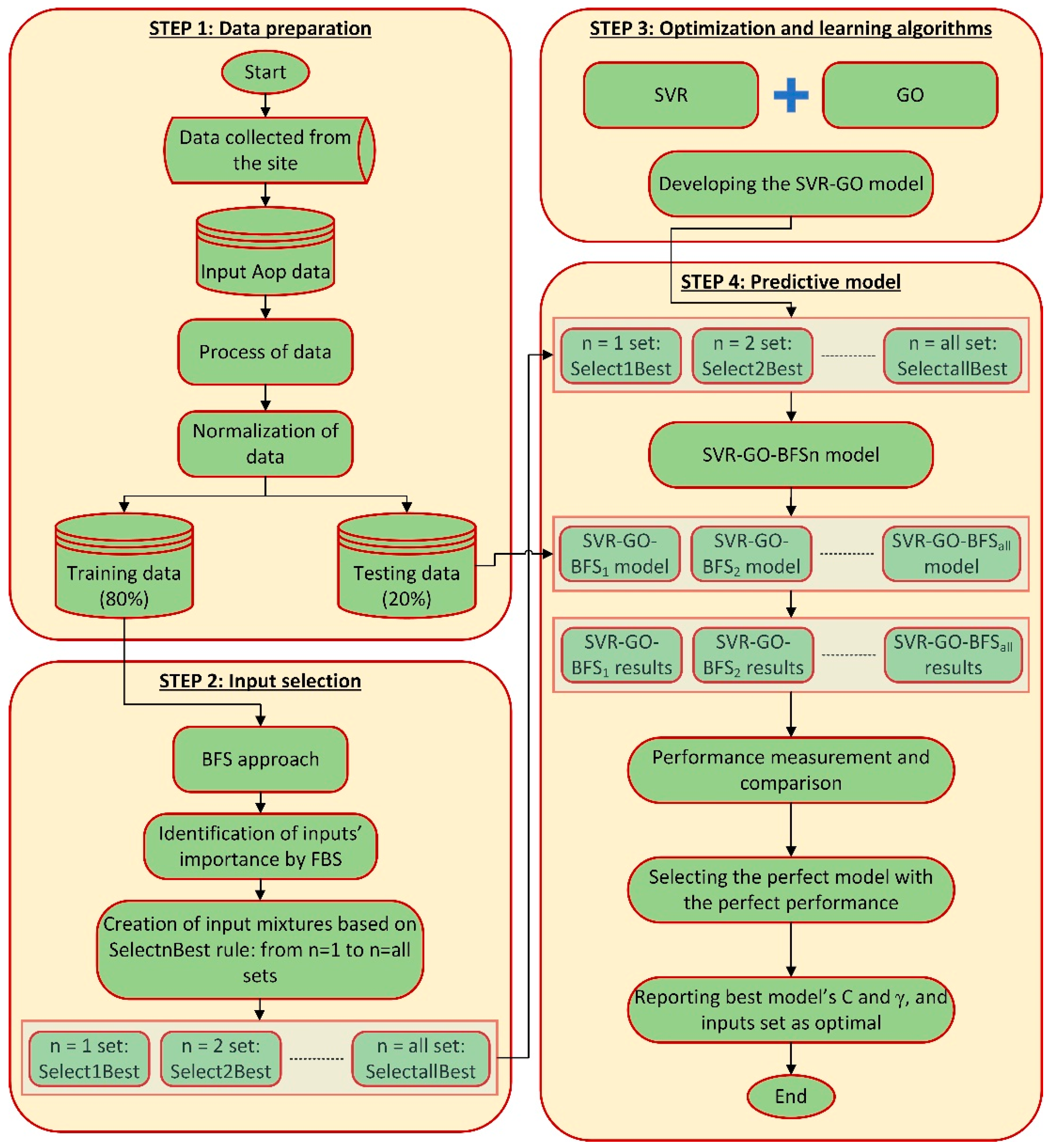
Following recognizing the importance level of the inputs by BFS, an SVR model kernelized with RBF is employed to carry out the predictive analysis. During running the model, γ and C that are pair hyperparameters of SVR are optimized by the GO algorithm. Nine SVR-GO-BFSn models (SVR-GO-BFS1 to SVR-GO-BFS9) are developed based on nine various inputs sets (n = 1 set to n = 9). The n = 1 set comprises just the first most significant input, while the n = 9 collection encompasses all nine vital inputs estimated by BFS. To choose among the SVR-GO-BFSn model structures, this study uses MAPE as the primary criterion. In addition, the RMSE is used as GO’s objective function. Prediction of the AOp values is the target of these models.
The AOp database is split into training (80%) and test (20%) sets at random throughout the experiment’s run. The training set of data is utilized to develop the forecasting model, while the testing data are utilized to evaluate the predictability. Importantly, all generated models receive the same training and test sets on a regular basis. Following building numerous models, it has been evidenced that as the number of iterations rises, the model computation time grows. Small population sizes, on the other hand, generate inconsistent fitness values. Therefore, multiple groups of 50, 100, 150, 200, and 250 population numbers in the optimization model were chosen for the purposes of the current study, and their iteration curves were made based on the right fitness values.
Concerning the GO, the number of search agents was set as 40, as well as the largest iteration number of developed models was set as 100. Regarding SVR, the lower and upper bounds of γ and C were set to (0.01–50) and (0.01, 100). All inputs were normalized between zero and one for the estimation of performance criteria, as well as to decrease the calculation complications during searching for hyperparameters of models. Table 3 presents the best predictive fulfilment of the models developed in the current investigation. This table corresponds to SVR hyperparameter values optimized using GO and the smallest optimal collection of inputs. It can be seen that the model with seven inputs (SVR-GO-BFS7) achieved the highest accuracy and lowest errors. 
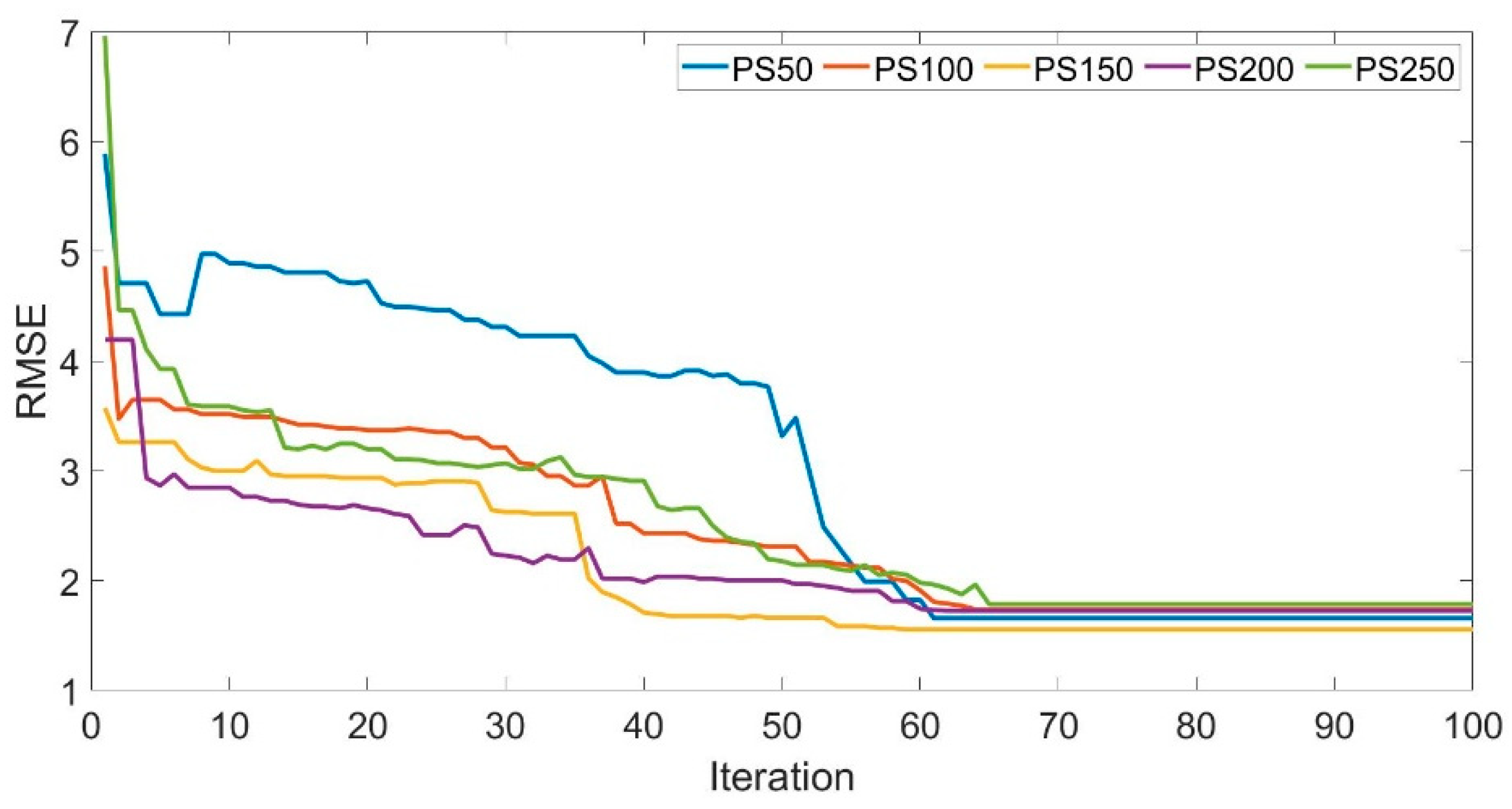
Figure 6 depicts the outcomes of fitness values for SVR-GO-BFS7 models in forecasting AOp, along with their iteration counts. Furthermore, to minimize the GO’s cost function, the RMSE was chosen. This figure shows that the best population size for SVR-GO-BFS7 is 200. Sizable errors in prediction are improbable to have occurred. Only average alternations were adopted up to iteration number 65; following this, no significant difference in the RMSE values was indicated. It should be noted that all models achieved the minimum RMSE in less than 70 iterations, which shows the power of GO in optimizing the SVR hyperparameters.
It was not required to have the full collection of significant inputs (n = nine) to obtain the most reliable predictive performance. Therefore, the authors can draw the conclusion that the effectiveness of SVR-GO-BFSn in forecasting the AOp is excellent.
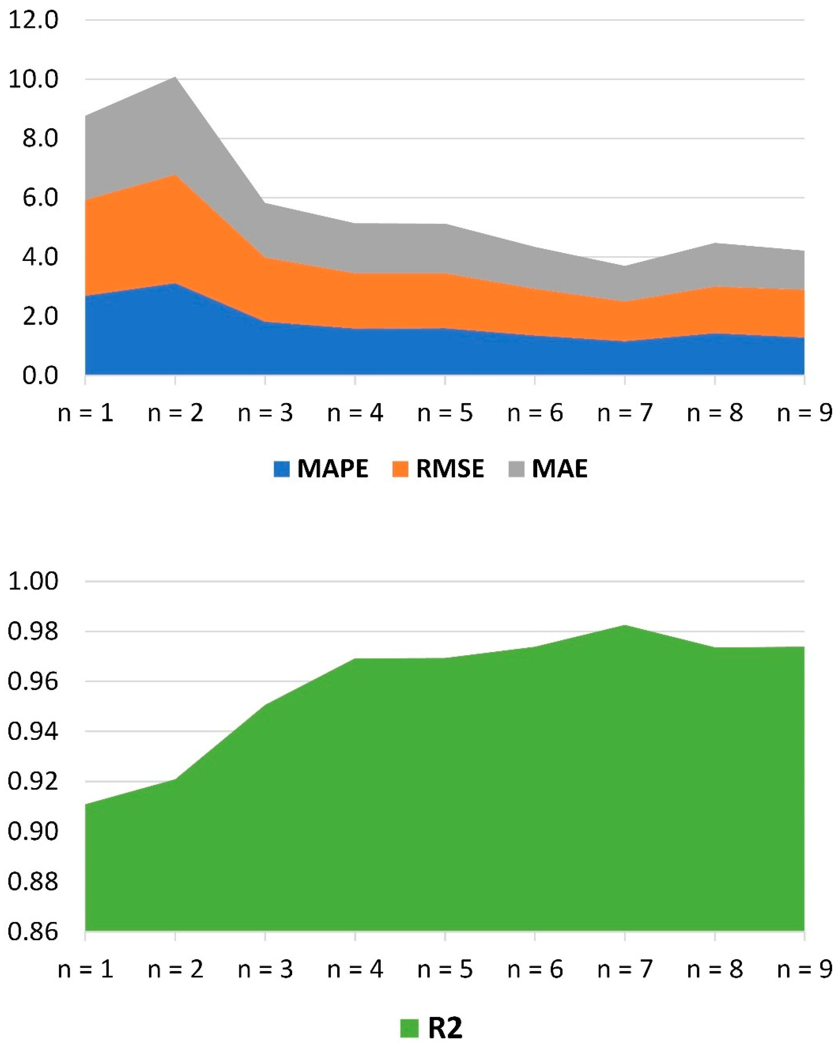
The performance of the SVR-GO-BFSn models based on various mixtures of significant inputs (n = 1 set to n = 9 sets) is presented in Figure 7 through the stacked area. In 
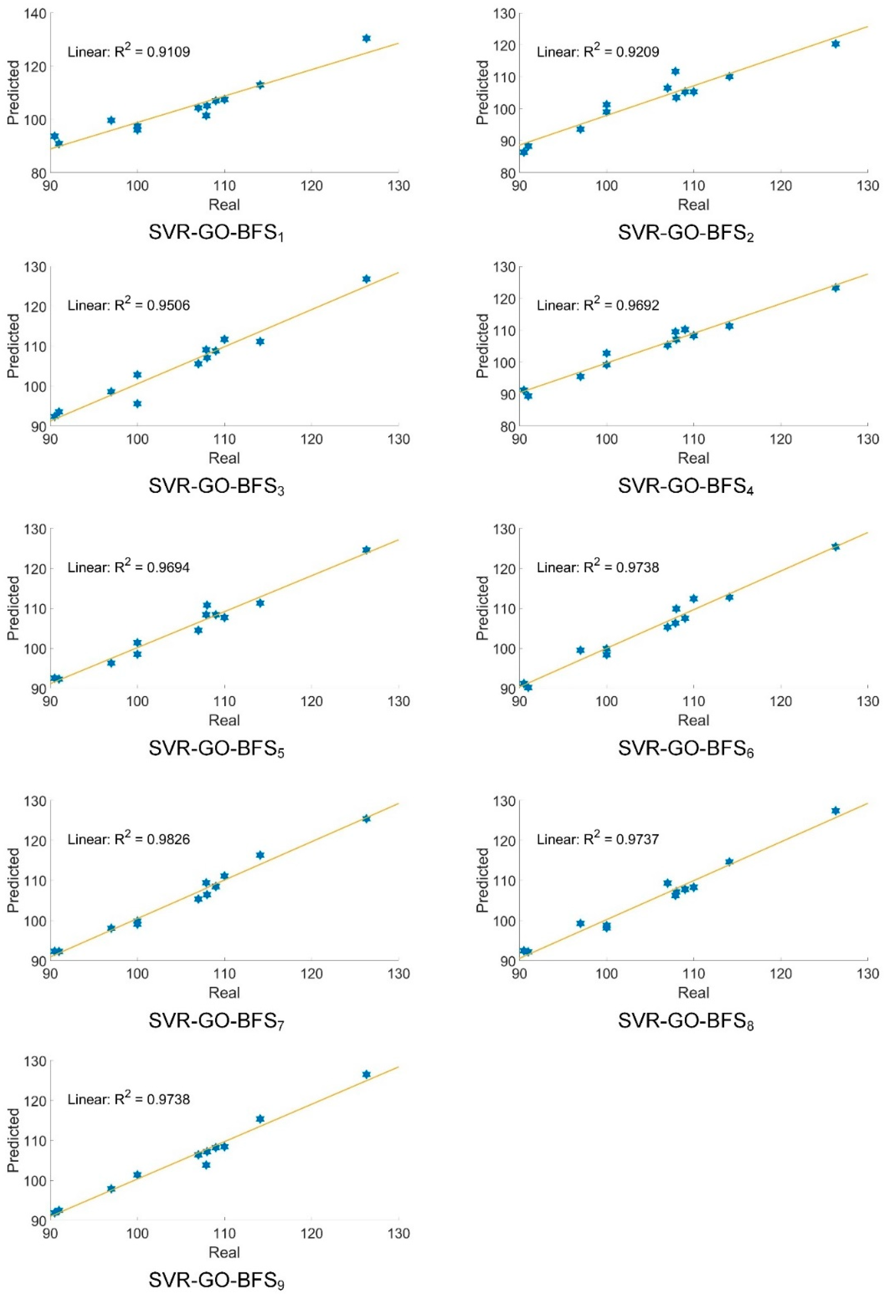
Figure 7, it is obvious that the MAPE, RMSE, and MAE estimates obtained from all the SVR-GO-BFSn models were essentially lower than 2.6953, 3.6637, and 3.3083, sequentially, even if only one input was added to the model. For instance, the achieved values of MAPE, RMSE, and MAE were 2.6953, 3.2241, and 2.8476, sequentially, if just one input is employed for the model creation. Furthermore, the SVR-GO-BFS2 model is associated with the poorest performance. This model achieved 0.9209 for R2, 36637 for RMSE, 3.1152 for MAPE, and 3.3083 for MAE. Instead, the developed models become more precise through employing the three most significant inputs and beyond. For instance, the acquired RMSE varied from 2.1659 to 1.6092 for the models from SVR-GO-BFS3 to SVR-GO-BFS9. Therefore, the authors can assume that employing just the three most significant inputs from the dataset picked and rated by BFS would produce strong prediction outcomes. Moreover, comparable issues were found with R2, MAPE, and MAE. The scatter plots of the real and predicted AOp values made by the developed models show this trend in Figure 8.

3.4. Performance Comparison

The authors compared the performance of the developed SVR-GO-BFS7 model with a single SVR model. All nine variables were used to train the single SVR model. The outcomes of this comparison are presented in Table 4. The SVR-GO-BFS7 model achieved a notably lower MAPE value compared with the single SVR model. The value of MAPE improved by about 62% when the newly developed model was applied to the data. Furthermore, R2 was enhanced by approximately 19%. RMSE and MAE were improved by 68.09% and 62.26%, respectively. Hence, for predictive precision, it can be assumed that SVR-GO-BFS7 particularly beats the single SVR model for AOp forecasting in the selected granite quarry sites in Malaysia. The principal responsible for enhancing the prediction performance of the SVR-GO-BFS7 model was SVR’s parameter optimization by GO and employing BFS for input choice.
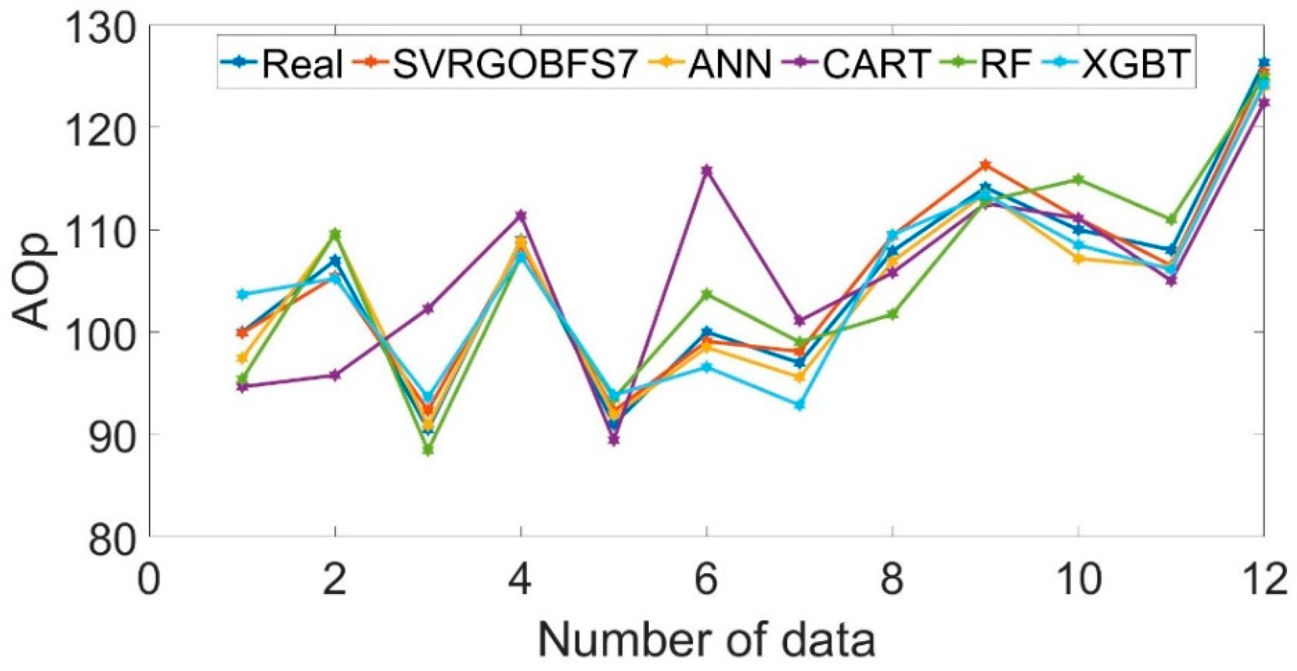
This study also compared the achievement of the developed model with some well-known ML models, including Random Forest (RF), Artificial Neural Networks (ANN), Extreme Gradient Boosting Tree (XGBT), and Classification and Regression Trees (CART). Nevertheless, BFS and GO were not hybridized with these models. All models were trained using the full set of inputs (nine inputs). For XGBT, Eta and Lambada were set as 0.3, 1.0, and its objective function was reg:linear. For CART, the maximum tree depth was 7. Concerning ANN, a backpropagation procedure by the Levenberg–Marquardt training algorithm was employed for its optimization. Additionally, the ANN structure included a single hidden layer and 11 hidden nodes. Furthermore, the authors used a sigmoid activation function while the value of the learning rate was 0.2. Table 5 shows how these models compare to SVR-GO-BFS7 in terms of how well they work.
The RMSE, MAPE, and MAE values of the developed SVR-GO-BFS7 model were less than all benchmark models. Among benchmark models, ANN showed a better performance in terms of both accuracy and errors. Instead, the worst model was CART, which achieved the lowest accuracy and highest errors. While the XGBT obtained better accuracy than the RF, the RF outperformed the XGBT in terms of errors. The results of this comparison confirmed that the developed SVR-GO-BFS
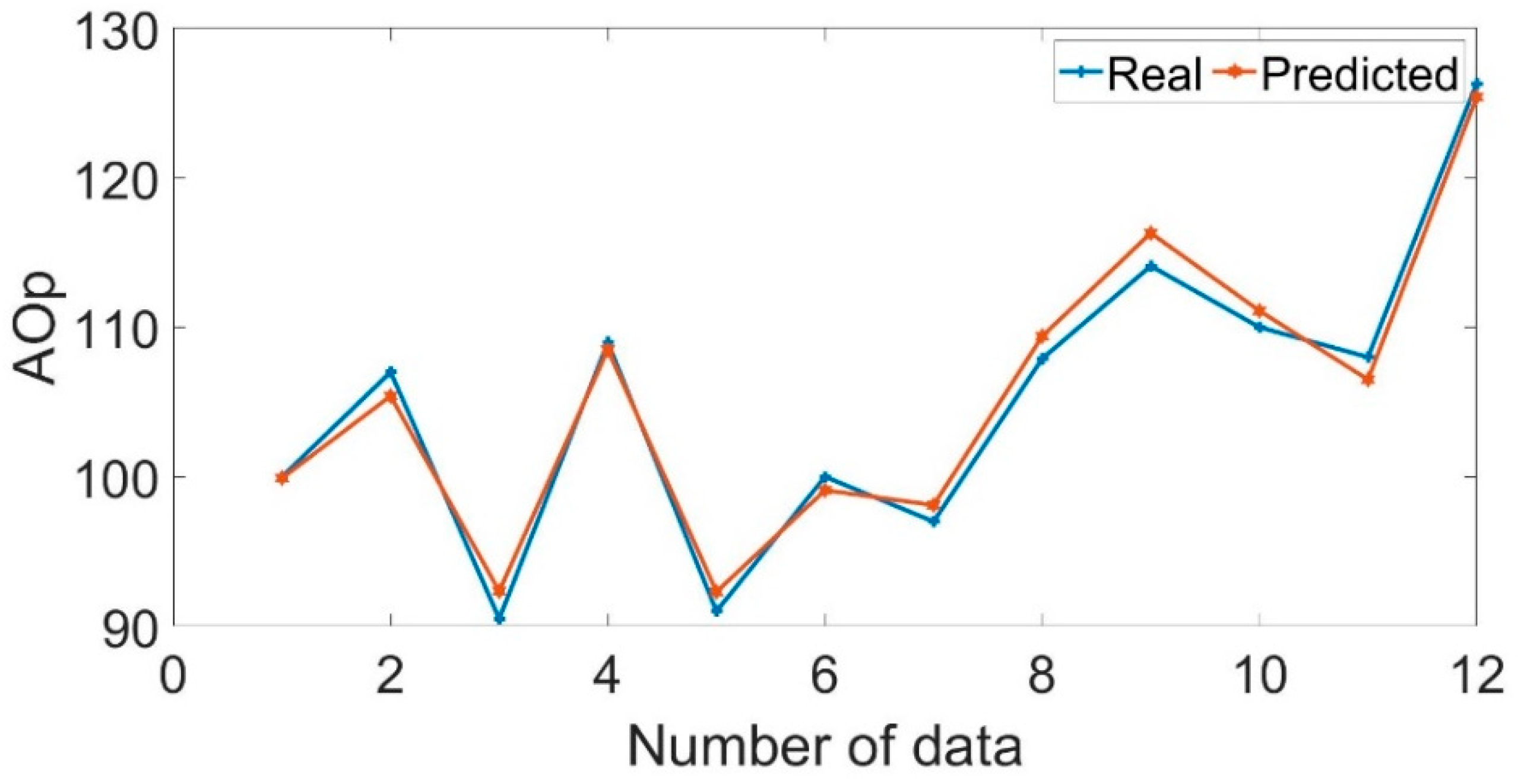
7 was statistically better than the models developed for comparison. For a better explanation, the predictive effectiveness of the developed BA-GO-BFS7 is demonstrated in Figure 9. The figure showed that the predicted data effectively track the real data with insignificant differences. The results of the performance criteria in Table 4 showed that the values of the error metrics were comparably low. The results of AOp predictions by SVR-GO-BFS7 and other ML models are presented in Figure 10. The advantage of the developed SVR-GO-BFS7 model was justified through the outcomes of the comparative evaluation. So, the importance of combining methods (SVR, GO, and BFS) is confirmed in the right way.

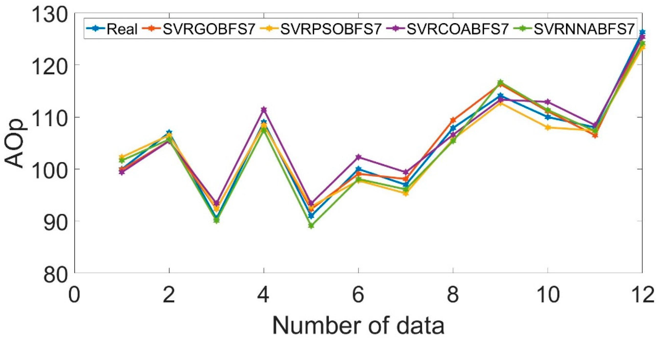
3.5. Comparison with Other Optimization Models

In the current section, various examinations were carried out to confirm that the synthesis of BFS, SVR, and GO produces the most reliable returns. This experiment engaged three optimizers to obtain the hyperparameters of SVR. One of these techniques was PSO, which explains the regular optimization performance for adjusting the SVR’s hyperparameters. Another method was the Cuckoo Optimization Algorithm (COA), which was broadly employed for fine-tuning the parameters of ML algorithms [38]. The last optimizer was the Neural Network Algorithm (NNA), one of the most advanced optimization techniques [39]. The SVR model was optimized with PSO, COA, and NNA. Seven of the inputs that SVR-GO-BFSn used were used again when the new optimized models were made.
The precision of the optimized models is presented in Figure 11. The performance results of the tuned SVR models by the optimized techniques are displayed in Table 6. For the granite quarry dataset, the precision of the SVR-GO-BFS7 model was higher than that of the SVR-PSO-BFS7, SVR-COA-BFS7, and SVR-NNA-BFS7 models. As a result, the capacity of the GO technique to search the SVR’s hyperparameters was more effective than NNA, PSO, and COA. Simply put, the SVR-GO-BFS7 method achieves high accuracy for AOp forecasting and has the best efficiency and consistency among all basic techniques. Overall, the SVR-GO-BFS7 technique obtained great precision for AOp prediction and had the greatest performance and cohesion amongst all basic methods. Consequently, in this research, the SVR-GO-BFSn model is used for prediction, and further studies are suggested to utilize this method in other investigations based on the authors’ concerns.
In comparison with the previous work, the model developed in this study showed better performance. For instance, Hajihassani et al. [27] applied an ANN-PSO to the same inputs, and they did not utilize any input selection technique and only used their model for AOp estimation. The best R2 that they achieved was 0.8836. The SVR-GA-BFS7 model achieved a better R2 while using a fewer number of inputs, which decreased the model complexity. The authors of this study believe that the current study and its process and results are able to add value to the available literature.

4. Conclusions and Future Works

Prediction of AOp values is vital because of their negative impacts on people and construction near the blasting zone. In this paper, a hybrid learning model, the SVR-GO-BFSn, was developed to forecast the AOp values. A summary of the significant findings of this study is provided below:
  • In incorporation with SVR, the BFS algorithm produced excellent forecasts on the dataset of this research concern.
  • The GO algorithm was confirmed to efficiently function in exploring the optimal conditions of SVR’s hyperparameters and achieving an accurate AOp prediction.
  • The reason for this efficacy was that this algorithm possesses a compelling ability for finding and controlling the optimal answers to multi-scale issues.
  • The developed model outperformed other established models in this study, including single SVR, CART, RF, ANN, and XGBT. Hence, the SVR-GO-BFSn can be a useful procedure for forecasting AOp values. Among the various optimizers used in this study, the GO optimizer outperformed the alternative ones, i.e., PSO, NNA, and COA.
As shown by the findings of the present study, the performance of the model developed was better than others. This approach is usable by other studies in different domains. Nevertheless, the regression issue is to be resolved by the developed model and is confined to the AOp forecast. Moreover, it is vital to note that the outcomes of this model are limited to quarries with similar characteristics. Although GO is a powerful optimizer, this study only used it to tune the SVR hyperparameters. We used only one dataset, which may be a limitation of this study. Future studies should use more datasets to test our proposed model.
Following this discussion, the authors suggest that further investigations could be carried out. Further studies should implement this developed method to deal with other issues in the blasting and mining analysis. Supplementary analysis of AOp predictions in various areas is required to assure the generalization of the outcomes of the developed system. The employment of GO as an input selection technique should be examined, and, subsequently, its efficiency should be analyzed against the BFS.

Author Contributions

L.C. Methodology, Software, Formal analysis, Writing—original draft. P.G.A. Methodology, Writing—review and editing, Supervision. M.Z.T. Writing—review and editing, Supervision. D.J.A., Conceptualization, Software, Formal analysis, Writing—review and editing, Supervision. D.V.U. Writing—review and editing. M.Y., Conceptualization, Writing—review and editing. All authors have read and agreed to the published version of the manuscript.

Funding

Supported by the Science and Technology Research Program of Chongqing Municipal Education Commission (Grant No. KJQN202103415).

Institutional Review Board Statement

Not applicable.

Informed Consent Statement

Not applicable.

Data Availability Statement

The data is available from the corresponding author upon reasonable request.

Conflicts of Interest

The authors declare no conflict of interest.

References

  1. Hagan, T.N. Rock breakage by explosives. In Gasdynamics of Explosions and Reactive Systems; Elsevier: Amsterdam, The Netherlands, 1980; pp. 329–340. [Google Scholar]
  2. Harandizadeh, H.; Armaghani, D.J. Prediction of air-overpressure induced by blasting using an ANFIS-PNN model optimized by GA. Appl. Soft Comput. 2020, 99, 106904. [Google Scholar] [CrossRef]
  3. Khandelwal, M.; Kankar, P. Prediction of blast-induced air overpressure using support vector machine. Arab. J. Geosci. 2011, 4, 427–433. [Google Scholar] [CrossRef]
  4. Konya CJ, W.E. Surface Blast Design; Prentice Hall: Englewood Cliffs, NJ, USA, 1990. [Google Scholar]
  5. Kuzu, C.; Fisne, A.; Ercelebi, S.G. Operational and geological parameters in the assessing blast induced airblast-overpressure in quarries. Appl. Acoust. 2009, 70, 404–411. [Google Scholar] [CrossRef]
  6. Wu, C.; Hao, H. Modeling of simultaneous ground shock and airblast pressure on nearby structures from surface explosions. Int. J. Impact Eng. 2005, 31, 699–717. [Google Scholar] [CrossRef]
  7. Rodríguez, R.; Toraño, J.; Menéndez, M. Prediction of the airblast wave effects near a tunnel advanced by drilling and blasting. Tunn. Undergr. Space. Technol. 2007, 22, 241–251. [Google Scholar] [CrossRef]
  8. Rodríguez, R.; Lombardía, C.; Torno, S. Prediction of the air wave due to blasting inside tunnels: Approximation to a ‘phonometric curve’. Tunn. Undergr. Space. Technol. 2010, 25, 483–489. [Google Scholar] [CrossRef]
  9. Hosseini, S.; Monjezi, M.; Bakhtavar, E.; Mousavi, A. Prediction of Dust Emission Due to Open Pit Mine Blasting Using a Hybrid Artificial Neural Network. Nat. Resour. Res. 2021, 30, 4773–4788. [Google Scholar] [CrossRef]
  10. Khandelwal, M.; Singh, T. Evaluation of blast-induced ground vibration predictors. Soil Dyn. Earthq. Eng. 2007, 27, 116–125. [Google Scholar] [CrossRef]
  11. Yang, H.; Song, K.; Zhou, J. Automated Recognition Model of Geomechanical Information Based on Operational Data of Tunneling Boring Machines. Rock Mech. Rock Eng. 2022, 55, 1499–1516. [Google Scholar] [CrossRef]
  12. Yang, H.; Wang, Z.; Song, K. A new hybrid grey wolf optimizer-feature weighted-multiple kernel-support vector regression technique to predict TBM performance. Eng. Comput. 2020, 38, 2469–2485. [Google Scholar] [CrossRef]
  13. Kardani, N.; Bardhan, A.; Samui, P.; Nazem, M.; Asteris, P.G.; Zhou, A. Predicting the thermal conductivity of soils using integrated approach of ANN and PSO with adaptive and time-varying acceleration coefficients. Int. J. Therm. Sci. 2022, 173, 107427. [Google Scholar] [CrossRef]
  14. Asteris, P.G.; Rizal, F.I.M.; Koopialipoor, M.; Roussis, P.C.; Ferentinou, M.; Armaghani, D.J.; Gordan, B. Slope Stability Classification under Seismic Conditions Using Several Tree-Based Intelligent Techniques. Appl. Sci. 2022, 12, 1753. [Google Scholar] [CrossRef]
  15. Barkhordari, M.; Armaghani, D.; Asteris, P. Structural Damage Identification Using Ensemble Deep Convolutional Neural Network Models. Comput. Model. Eng. Sci. 2022. [Google Scholar] [CrossRef]
  16. Asteris, P.G.; Lourenço, P.B.; Roussis, P.C.; Adami, C.E.; Armaghani, D.J.; Cavaleri, L.; Chalioris, C.E.; Hajihassani, M.; Lemonis, M.E.; Mohammed, A.S. Revealing the nature of metakaolin-based concrete materials using artificial intelligence techniques. Constr. Build. Mater. 2022, 322, 126500. [Google Scholar] [CrossRef]
  17. Zhou, J.; Qiu, Y.; Khandelwal, M.; Zhu, S.; Zhang, X. Developing a hybrid model of Jaya algorithm-based extreme gradient boosting machine to estimate blast-induced ground vibrations. Int. J. Rock Mech. Min. Sci. 2021, 145, 104856. [Google Scholar] [CrossRef]
  18. Zhou, J.; Dai, Y.; Khandelwal, M.; Monjezi, M.; Yu, Z.; Qiu, Y. Performance of Hybrid SCA-RF and HHO-RF Models for Predicting Backbreak in Open-Pit Mine Blasting Operations. Nat. Resour. Res. 2021, 30, 4753–4771. [Google Scholar] [CrossRef]
  19. Zhou, J.; Chen, C.; Wang, M.; Khandelwal, M. Proposing a novel comprehensive evaluation model for the coal burst liability in underground coal mines considering uncertainty factors. Int. J. Min. Sci. Technol. 2021, 31, 799–812. [Google Scholar] [CrossRef]
  20. Zhang, R.; Li, Y.; Gui, Y.; Zhou, J. Prediction of blasting induced air-overpressure using a radial basis function network with an additional hidden layer. Appl. Soft Comput. 2022, 127, 109343. [Google Scholar] [CrossRef]
  21. Zeng, J.; Jamei, M.; Nait Amar, M.; Hasanipanah, M.; Bayat, P. A novel solution for simulating air overpressure resulting from blasting using an efficient cascaded forward neural network. Eng. Comput. 2022, 38, 2069–2081. [Google Scholar] [CrossRef]
  22. Hosseini, S.; Poormirzaee, R.; Hajihassani, M. Application of reliability-based back-propagation causality-weighted neural networks to estimate air-overpressure due to mine blasting. Eng. Appl. Artif. Intell. 2022, 115, 105281. [Google Scholar] [CrossRef]
  23. Hasanipanah, M.; Jahed Armaghani, D.; Khamesi, H.; Bakhshandeh Amnieh, H.; Ghoraba, S. Several non-linear models in estimating air-overpressure resulting from mine blasting. Eng. Comput. 2016, 32, 441–455. [Google Scholar] [CrossRef]
  24. Murlidhar, B.; Bejarbaneh, B.; Armaghani, D.; Mohammed, A.; Mohamad, E. Application of Tree-Based Predictive Models to Forecast Air Overpressure Induced by Mine Blasting. Nat. Resour. Res. 2020, 30, 1865–1887. [Google Scholar] [CrossRef]
  25. Hasanipanah, M.; Shahnazar, A.; Bakhshandeh Amnieh, H.; Jahed Armaghani, D. Prediction of air-overpressure caused by mine blasting using a new hybrid PSO–SVR model. Eng. Comput. 2017, 33, 23–31. [Google Scholar] [CrossRef]
  26. He, Z.; Armaghani, D.J.; Masoumnezhad, M.; Khandelwal, M.; Zhou, J.; Murlidhar, B.R. A Combination of Expert-Based System and Advanced Decision-Tree Algorithms to Predict Air—Overpressure Resulting from Quarry Blasting. Nat. Resour. Res. 2021, 30, 1889–1903. [Google Scholar] [CrossRef]
  27. Hajihassani, M.; Jahed Armaghani, D.; Sohaei, H.; Tonnizam Mohamad, E.; Marto, A. Prediction of airblast-overpressure induced by blasting using a hybrid artificial neural network and particle swarm optimization. Appl. Acoust. 2014, 80, 57–67. [Google Scholar] [CrossRef]
  28. Vapnik, V. The Nature of Statistical Learning Theory; Springer Science & Business Media: Berlin, Germany, 2013; ISBN 1475732643. [Google Scholar]
  29. Dreyfus, G. Neural Networks: Methodology and Applications; Springer: Berlin/Heidelberg, Germany, 2005. [Google Scholar]
  30. Saremi, S.; Mirjalili, S.; Lewis, A. Grasshopper optimisation algorithm: Theory and application. Adv. Eng. Softw. 2017, 105, 30–47. [Google Scholar] [CrossRef]
  31. Kursa, M.B.; Rudnicki, W.R. Feature selection with the Boruta package. J. Stat. Softw. 2010, 36, 1–13. [Google Scholar] [CrossRef]
  32. Lu, S.; Koopialipoor, M.; Asteris, P.G.; Bahri, M.; Armaghani, D.J. A Novel Feature Selection Approach Based on Tree Models for Evaluating the Punching Shear Capacity of Steel Fiber-Reinforced Concrete Flat Slabs. Materials 2020, 13, 3902. [Google Scholar] [CrossRef]
  33. Asteris, P.G.; Argyropoulos, I.; Cavaleri, L.; Rodrigues, H.; Varum, H.; Thomas, J.; Lourenço, P.B. Masonry compressive strength prediction using artificial neural networks. In Proceedings of the International Conference on Transdisciplinary Multispectral Modeling and Cooperation for the Preservation of Cultural Heritage, Athens, Greece, 10–13 October 2018; pp. 200–224. [Google Scholar]
  34. Huang, J.; Asteris, P.; Pasha, S.; Mohammed, A.; Hasanipanah, M. A new auto-tuning model for predicting the rock fragmentation: A cat swarm optimization algorithm. Eng. Comput. 2020, 38, 2209–2220. [Google Scholar] [CrossRef]
  35. Asteris, P.G.; Gavriilaki, E.; Touloumenidou, T.; Koravou, E.; Koutra, M.; Papayanni, P.G.; Pouleres, A.; Karali, V.; Lemonis, M.E.; Mamou, A. Genetic prediction of ICU hospitalization and mortality in COVID-19 patients using artificial neural networks. J. Cell. Mol. Med. 2022, 26, 1445–1455. [Google Scholar] [CrossRef]
  36. Asteris, P.G.; Douvika, M.G.; Karamani, C.A.; Skentou, A.D.; Chlichlia, K.; Cavaleri, L.; Daras, T.; Armaghani, D.J.; Zaoutis, T.E. A novel heuristic algorithm for the modeling and risk assessment of the COVID-19 pandemic phenomenon. Comput. Model. Eng. Sci. 2020, 125, 815–828. [Google Scholar] [CrossRef]
  37. Psyllaki, P.; Stamatiou, K.; Iliadis, I.; Mourlas, A.; Asteris, P.; Vaxevanidis, N. Surface treatment of tool steels against galling failure. In Proceedings of the MATEC Web of Conferences; EDP Sciences: Les Ulis, France, 2018; Volume 188, p. 4024. [Google Scholar]
  38. Rajabioun, R. Cuckoo optimization algorithm. Appl. Soft Comput. 2011, 11, 5508–5518. [Google Scholar] [CrossRef]
  39. Sadollah, A.; Sayyaadi, H.; Yadav, A. A dynamic metaheuristic optimization model inspired by biological nervous systems: Neural network algorithm. Appl. Soft Comput. 2018, 71, 747–782. [Google Scholar] [CrossRef]
Figure 1. The SVR’s structure SVR.
Applsci 12 09805 g001
Figure 2. The execution steps of BFS.
Applsci 12 09805 g002
Figure 3. Flowchart of this study.
Applsci 12 09805 g003
Figure 4. 10-fold cross validation schematic view.
Applsci 12 09805 g004
Figure 5. The results of the input selection study on the data.
Applsci 12 09805 g005
Figure 6. SVR-GO-BFS7 optimization model for different population sizes (PSs).
Applsci 12 09805 g006
Figure 7. Performance of the SVR-GO-BFSn models with various inputs.
Applsci 12 09805 g007
Figure 8. Real and predicted AOp values by various developed models, SVR-GO-BFS7 is the best model.
Applsci 12 09805 g008
Figure 9. Real and predicted AOp values.
Applsci 12 09805 g009
Figure 10. Results of predictions by various models.
Applsci 12 09805 g010
Figure 11. The outcomes of the developed model with various optimization methods.
Applsci 12 09805 g011
Table 1. Some additional measurements in blasting sites.
SiteRQD (%)Height of Bench (m)
Masai60–8415–20
Pasir Gudang67–8913–25
Pengerang70–9110–23
Ulu Tiram65–8810–15
Table 2. Implementation steps of GO algorithm.
1st STEP A i = j = 1 , j i N a ( f i j ) · f i j ^
  • fij is a space, which divides the ith and jth grasshoppers, fij = |aj − ai|
  • fij = (ai − aj)/fij means the unit vector between the ith and jth grasshoppers
(7)
a ( m ) = z · e m d e m
  • z is the attraction intensity
  • d signifies the attractive length scale
  • m = |dij|
(8)
2nd STEP B i = b · e b
  • b is gravitational constant
  • eb stands for the unit vector heading to the globe center
(9)
3rd STEP C i = x · e ω
  • x is a constant drift
  • eω refers to a unity vector in the wind direction
  • N signifies the grasshoppers’ number
(10)
Y i = j = 1 , j i N b ( | a j a i | ) · a j a i f i j t · e t + x · e ω (11)
Y i f = c ( j = 1 , j i N c · u b d d b f 2 · a ( | a j d a i d | ) · a j a i f i j ) + O f
  • dbf and ubd are lower and upper boundaries in the Fth dimension
  • Of is the location of the optimum solution it has found yet
(12)
c = c m a x d · c m a x c m i n D
  • cmin and cmax refers to the minimum and the maximum values of the coefficient c
  • d implies the existing iteration
  • D represents the greatest iterations
(13)
Table 3. Best model performance.
Performance Criterion
Best modelSVR-GO-BFS7
Inputs No.7
R20.9826
RMSE1.3315
MAE1.2108
MAPE1.1633
C9.3119
γ0.6363
Table 4. Performance comparison between single SVR and SVR-GO-BFS7.
Performance CriterionSVR-GO-BFS7Single SVR
R20.98260.8245
RMSE1.33154.1728
MAE1.21083.2083
MAPE1.16333.0527
Table 5. Comparison between the SVR-GO-BFS7 and other models.
Performance CriterionSVR-GO-BFS7ANNCARTRFXGBT
R20.98260.97670.51920.88740.9342
RMSE1.33151.72067.07003.33002.5632
MAE1.21081.47675.31682.98082.3600
MAPE1.16331.39275.24272.86922.3240
Table 6. Comparison of various optimizers for AOp prediction.
Performance CriterionSVR-GO-BFS7SVR-PSO-BFS7SVR-COA-BFS7SVR-NNA-BFS7
R20.98260.97960.97290.9747
RMSE1.33151.81881.95471.6929
MAE1.21081.66751.74751.5625
MAPE1.16331.59971.71701.4740
Publisher’s Note: MDPI stays neutral with regard to jurisdictional claims in published maps and institutional affiliations.

