Control Strategy of Speed Segmented Variable Constant Power Powertrain of Electric Construction Machinery

Abstract

Energy conservation and emission reduction have become a global development consensus. Traditional construction machinery driven by an engine has high energy consumption and poor emission. Electric construction machinery is considered to be one of the main trends in the future due to its zero emissions by canceling the engine and using the motor-driven hydraulic system. However, most of the existing electric construction machinery works through the motor to simulate the engine without considering the regulation characteristics of the motor. Therefore, although the existing electric construction machinery improves the emission and the energy efficiency of the power system to a certain extent, the control of the motor and hydraulic systems can still be further optimized. The energy efficiency of the whole machine can be maximized. Based on the LUDV system of construction machinery, a control strategy based on motor speed classification and variable constant power can automatically identify the actual working conditions of the electric excavator and adjust the starting pressure of the constant power valve, to change the constant power range of hydraulic pump and achieve the goal of adapting to the working conditions of power system, is proposed. Simulation and experiments are carried out to verify the feasibility of the proposed control strategy. The results show that the speed classification and variable constant power control system can effectively realize the hierarchical regulation of motor speed and provide relatively stable speed input for the hydraulic system. Moreover, the current working condition can be identified through the pump outlet pressure. The adaption of the working conditions can be realized through the proportional reducing valve by adjusting the starting pressure of the variable constant power valve.

1. Introduction

Energy conservation and emission reduction have become a global development consensus [1,2]. Construction machinery is widely used, but it has the shortcomings of low energy efficiency and poor emissions [3]. Taking the traditional 20 t excavator as an example, the energy efficiency of the power system and the hydraulic system are only about 35% [4]. It is urgent to carry out research on energy conservation and emission reduction technologies for construction machinery [5,6].

At present, energy-saving research is mainly focus on the power system and the hydraulic system [7]. The research on power system energy-saving technologies can be divided into energy-saving technologies based on the traditional engine, hybrid power technologies and pure electric technologies. The energy-saving technology based on the traditional engine mainly improves the fuel injection characteristics of the engine through electronic control, so as to improve the diesel combustion efficiency. While, energy-saving technologies based on the traditional engine can be further divided into working condition division control, automatic idle control, constant power control [8,9,10] and cylinder deactivation control [11]. However, due to the bottleneck of engine development, it is difficult to further improve the energy efficiency. The hybrid power system mainly uses the auxiliary power source to drive the load together with the engine and stabilize the engine working point, to improve the energy efficiency of the engine. However, the configuration and control of the hybrid power system are complicated. Moreover, the engine is employed in hybrid power technologies. The improvement in energy efficiency and emission are still unsatisfactory [12,13]. Electric construction machinery uses a motor to replace the engine, in which high energy efficiency and zero emission can be achieved. It is considered to be one of the important trends in the development of construction machinery [14,15,16].

At present, some research has been carried out on electric construction machinery. Some machine manufacturers, including Komatsu, Doosan, Sunward, XCMG, SANY, Liebherr, and Caterpillar, have launched electric construction machinery. However, the electrification technology for construction machinery is still in its infancy. Most electric construction machineries use motors to replace engines and simulate the working mode of engines. The working characteristics of the hydraulic system are not fully considered, which leads to the limited comprehensive matching characteristics of the motor and hydraulic system. At present, many scholars have carried out research on the electrification of construction machinery.

Quan et al. used a variable speed motor to drive the pump in a hydraulic system for flow matching. The energy consumption of the power system was reduced from 2.05 to 0.7 kW. The energy-saving efficiency was up to 33%. Compared with traditional excavators, the energy consumption of the whole machine could be saved by more than 30% [17,18]. Lin et al. used a motor to replace the engine and proposed a two-stage idle speed control system for an electric excavator with an accumulator [19]. The results showed that the fast response during mode switching could be realized. Moreover, the energy-saving efficiency of the system was about 36.06% [20]. Yoon et al. carried out research on the electric excavator based on the electro-hydraulic actuator. The integrations of driving and regeneration for the potential energy and the kinetic energy of the excavator boom and swing were achieved, respectively. A 5 t excavator test prototype was developed [21]. Similar research was carried out by Minav et al. as well. Three independent motor pumps were used for the boom, arm, and bucket of a 1 t excavator. The results showed that in the selected typical working condition, the efficiency of the system was 71.3% [22].

At present, electrification technologies have been widely used in the field of automobile, but their applications to construction machinery are still in their infancy. Because of significant differences between construction machinery and automobile in structure, working condition, load and working environment, the research on electrification technology of construction machinery needs to be reconsidered.

Based on the LUDV system, to give full play to the excellent speed regulation characteristics of the motor, the research on the flow matching technology through variable speed motor-variable displacement pump for excavator is studied. Meanwhile, the flow prediction for multi-actuators pilot signals is realized, so as to further improve the system efficiency and the controllability.

2. Preliminary Consideration

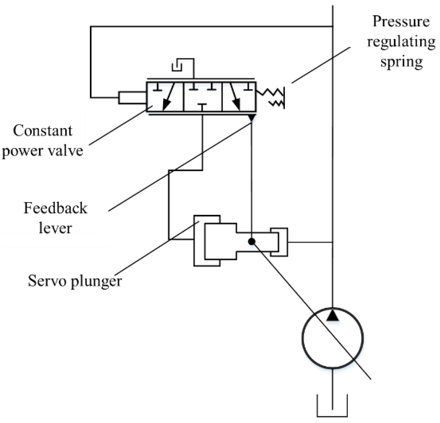
In the traditional excavator based on engine, the speed of engine is preset and fixed during operation. To match the operation requirements of different working conditions and improve the absorption rate of the hydraulic pump from the engine output power, the constant power control is employed to limit the hydraulic system output power and match the output power of power source. The constant power control is adjusted through the displacement regulation mechanism of pump. The structural principle diagram of the constant power regulation system is given in Figure 1.

The constant power valve is a three-position and three-way directional valve. The valve sleeve is connected with the piston of the pump displacement variable mechanism. The left end of the constant pressure valve core is connected with the pump outlet pressure signal P_p. Two springs are equipped at the right end, with lengths of L₁ and L₂, respectively, where L₁ > L₂ and elastic coefficients are k₁ and k₂, respectively. The initial state of spring 1 is compressed. The initial set pressure of spring 1 is P₁. The spring 2 is naturally extended without pressure.

When P_p < P₁, the constant power valve spool moves to the left. The constant power valve works in the right position. The oil chamber at the left end of the variable piston returns to the oil tank. The variable piston moves to the left. The variable pump works at the maximum displacement.

When P_p = P₁, the constant power valve works in the middle position. The oil chamber at the left end of the variable piston is closed. The piston displacement remains unchanged, and the variable pump still works at the maximum displacement.

When P_p > P₁, the constant power valve core moves to the right. The constant power valve works in the left position. The oil chamber at the left end of the variable piston is connected to the pump outlet. Suppose the left end cross-sectional area of the variable piston is S₁ and the right end cross-sectional area of the variable piston is S₂, and S₁ > S₂. The forces on the left and right ends of the variable piston can be expressed as

$$T_1=P_{\mathrm{p}}{S}_1>P_{\mathrm{p}}{S}_2=T_2$$

(1)

where T₁ is the force of the variable piston left end. T₂ is the force of the variable piston right end. P_p is the output pressure of the pump. S₁ is the left end cross-sectional area. S₂ is the right end cross-sectional area.

The variable displacement piston moves to the right to reduce the displacement of the pump. Meanwhile, the variable piston moving to the right drives the constant power valve sleeve to the right through the connecting rod so that the constant power valve works in the middle position again. The variable pump maintains the current displacement. The compression displacement of spring 1 is ∆x₁, and the cross-sectional area of the left end of the valve core is S₃. At this time, the balance formula of the constant power valve core can be given as

$$P_{\mathrm{p}}{S}_3=P_1{S}_3+k_1\Delta x_1$$

(2)

where S₃ is the area of the left end of the constant power valve core. P₁ is the initial set pressure of spring 1. k₁ is the elastic coefficients of spring 1. ∆x₁ is the compression displacement of spring 1.

When the load pressure continues to rise, causing the rise of pump outlet pressure P_p. The constant power valve continues to repeat the above steps. The displacement of the variable pump decreases with the increase in the pump outlet pressure until the valve core of the constant power valve contacts the spring 2. The compression displacement of spring 2 is ∆x₂. At this time, spring 1 and spring 2 act together on the right side of the constant power valve spool. The elastic coefficient of these two springs is k₁ + k₂. The above changes continually with the pump outlet pressure at the left end of the constant power valve spool. The displacement of the variable pump decreases with the increase in the pump outlet pressure. At this time, the balance formula of the spool can be deduced as

$$P_{\mathrm{p}}{S}_3=P_1{S}_3+k_1\Delta x_1+(k_1+k_2)\Delta x_2$$

(3)

where k₂ is the elastic coefficients of spring 2. ∆x₂ is the compression displacement of spring 2.

Until the displacement of variable displacement pump is adjusted to the minimum displacement. Because the pump displacement changes with the pump outlet pressure, the constant power valve spool works in the process from one spring to two springs, and the spring elasticity coefficient changes, which affects the slope of the pump displacement changing with the pump outlet pressure. When the input speed of the pump is constant. The variation curve of the pump outlet flow with the pump outlet pressure is shown in Figure 2.

As can be seen, the approximate constant power control is realized by changing the spring stiffness. The pump enters the constant power mode from point A. The pressure at point A depends on the starting pressure set by the spring 1. Starting from point B, the constant power enters the second stage, which is adjusted by the springs 1 and 2. The fitting curve of approximate constant power can be obtained by the joint action of two springs. After entering the constant power point of the pump, the displacement of the variable pump varies linearly with the displacement of the valve core of the constant power valve, which can be expressed as

$$\Delta V=\lambda \Delta x$$

(4)

where ∆V is the variation of the displacement of the pump. λ is the scale factor. ∆x is the displacement of the valve core of the constant pressure valve.

When the pump operates in the section AB, the flow of the pump can be given as

$$Q=Q_{\max }-\Delta Q=(V_{\max }-\Delta V)n$$

(5)

where Q is the output flow of the pump. Q_max is the maximum flow of the pump. ΔQ is the reduced flow of the pump due to the reduction in displacement of the pump. V_max is the maximum displacement of the pump. ΔV is the reduction in displacement of the pump. n is the speed of the pump.

Combined Equations (2) and (5), the relationship between outlet flow Q and pressure P_p of the pump in section AB can be deduced as

$$Q=-\raisebox{1ex}{$\lambda n{S}_3$}\!\left/ \!\raisebox{-1ex}{$k_1$}\right.P_{\mathrm{p}}+(n{V}_{\max }+\raisebox{1ex}{$\lambda n{P}_1{S}_3$}\!\left/ \!\raisebox{-1ex}{$k_1$}\right.)$$

(6)

The constant value in Equation (6) is defined as

$$\{\begin{array}{l}{K}_1=\frac{\lambda n{S}_3}{k_1}\\ C_1=n{V}_{\max }+\frac{\lambda n{P}_1{S}_3}{k_1}\end{array}$$

(7)

Combined Equations (6) and (7), the relationship between outlet flow Q and pressure P_p of pump in section AB can be re-expressed as

$$Q=-K_1{P}_{\mathrm{p}}+C_1$$

(8)

Through Equation (6), when the hydraulic pump enters the AB stage of constant power operation of the pump from point A, the pump outlet flow Q has a negative linear relationship with the pressure P_p, and the slope is −K₁.

In the section BC, the displacement of the core valve of the constant pressure valve is ∆x₁. The further movement displacement of the core valve of the constant pressure valve is ∆x₂. Combine Equation (4), the outlet flow of the pump can be given as

$$Q=-K_1{P}_{\mathrm{p}}+C_1$$

(9)

Combine Equations (3) and (5), the relationship between outlet flow Q and pressure P_p of pump in section AB can be deduced as

$$Q=\frac{\lambda n{S}_3}{k_1+k_2}{P}_{\mathrm{p}}+(n{V}_{\max }+\frac{\lambda n(P_1{S}_3+k\Delta x_1)}{k_1+k_2}-\lambda n\Delta x_1)$$

(10)

The constant value in Equation (10) is defined as

$$\{\begin{array}{l}{K}_2=\frac{\lambda n{S}_3}{k_1+k_2}\\ C_2=n{V}_{\max }+\frac{\lambda n(P_1{S}_3+k_1\Delta x_1)}{k_1+k_2}-\lambda n\Delta x_1\end{array}$$

(11)

Combined Equations (10) and (11), the relationship between outlet flow Q and pressure P_p of pump in section AB can be re-expressed as

$$Q=-K_2{P}_{\mathrm{p}}+C_2$$

(12)

According to Equation (12), when the hydraulic pump enters the BC stage of constant power operation of the pump from point B, the pump outlet flow Q has a negative linear relationship with the pressure P_p, and the slope is −K₂. Because |K₁| > |K₂|, the curve of section AB has a greater inclination than that of section BC.

Therefore, the constant power valve is fed back through the pump outlet pressure and compared with the starting pressure set by the spring at the right end of the constant power valve spool to determine the initial system pressure of the variable pump entering the constant power operation stage. By connecting the constant power valve sleeve with the variable piston of the variable pump, balancing the spring force with the pump outlet pressure, and cooperating with the spring variable stiffness structure, the approximate constant power control can be realized.

3. Control Strategy of Variable Displacement Pump under Different Working Conditions

The load sensing pump meets the load requirement under different working conditions through the constant power valve and the power source. The schematic diagram of the load sensing pump is shown in Figure 3.

The load sensing variable displacement pump is composed of constant power valve, load sensing valve (LS valve), pressure cut-off valve, electric proportional reducing valve, variable pressure thimble and variable piston. The left end of the constant power valve core is connected to the pump outlet pressure P_p, which acts simultaneously with the variable pressure thimble. The oil inlet of the variable pressure thimble oil chamber is controlled by the electric proportional reducing valve, which can change the hydraulic thimble pressure F₄ by controlling the electric proportional reducing valve through the electric signal. The right end of the valve core of the constant power valve is a constant power starting spring, and the starting force of the spring 1 is set as F₁. The other short spring is a secondary spring, which is not in contact with the right end of the valve core directly. The left end of the load LS valve is connected with the maximum load pressure P_L, which acts on the left end of the valve core at the same time as the spring 2. Set the spring 2 force as F₂, and the right end of the valve core introduces the pump outlet pressure P_p. A spring 3 is arranged at the left end of the pressure cut-off valve, the spring force is set as F₃. The pump outlet pressure P_p is connected with the right end of the valve core. The cross-sectional areas of constant power valve, LS valve and pressure cut-off valve cores are set as A₁, A₂ and A₃, respectively. The spring force relationship is F₂ < F₁ < F₃. The hydraulic pump input speed is considered as constant.

3.1. Non Constant Power Stage

As shown in Figure 2, in section MA, the load in this stage is small. The system has not entered the constant power operation stage. The left end of the LS valve core is connected with the maximum load pressure P_L, which is affected by the spring force F₁. The right end is connected with the pump outlet pressure P_p. The balance equation for the LS valve is obtained as Equation (13). LS valve ensures that the pump outlet pressure is always greater than the maximum load by a target value, which can be expressed as P_LS = F₂/A₂.

$$\begin{array}{l}{P}_{\mathrm{L}}{A}_2+F_2=P_{\mathrm{p}}{A}_2\\ P_{\mathrm{p}}=P_{\mathrm{L}}+\frac{F_2}{A_2}\end{array}$$

(13)

where P_L is the maximum pressure of load. F₂ is the spring 2 force. A₂ is the left end area of LS valve.

The left end of the constant power valve core is connected with the pump outlet pressure. At the same time, it is under the action of variable pressure thimble. Set the pressure of the oil chamber of the variable thimble as P_f, which is determined by the current I of the input electric proportional reducing valve. Set the cross-sectional area of the thimble oil chamber as S. The force relationship of constant valve core can be deduced as (14). The constant power valve works in the right position.

$$\begin{array}{l}{P}_{\mathrm{f}}S+P_{\mathrm{p}}{A}_1<F_1\\ P_{\mathrm{f}}=f(I)\end{array}$$

(14)

where P_f is the pressure of the oil chamber of the variable thimble. S is the left end area of constant power valve. F₁ is the starting force of the spring 1. f() is the function between the pressure of the oil chamber and input current. I is the input current of reducing valve.

The left end of the pressure cut-off valve spool is affected by the spring force F₃. The right end is connected with the pump outlet oil circuit. At this time, the force relationship of the left and right ends of the pressure cut-off valve spool is deduced as (15). The pressure cut-off valve works in the left position.

$$F_3>P_{\mathrm{p}}{A}_3$$

(15)

where F₃ is the spring force of the left end of the pressure cut-off valve. A₃ is the area of cut valve.

In this working stage, the oil chamber at the left end of the variable piston returns to the oil tank through the pressure cut-off valve, LS valve and constant power valve. The variable piston moves left to the maximum displacement, and the pump displacement works at the maximum displacement. With the increase in the pump outlet pressure, the pump displacement remains unchanged.

3.2. Constant Power Stage

When the system pressure continues to rise until it reaches the starting pressure of the constant power valve, the hydraulic system enters the constant power operation stage, as can be seen point A in Figure 2. At this time, the left and right balance equation of the constant power valve spool can be expressed as

$$\begin{array}{l}{P}_{\mathrm{f}}S+P_{\mathrm{p}}{A}_1>F_1\\ P_{\mathrm{p}}>\frac{F_1-P_{\mathrm{f}}S}{A_1}\end{array}$$

(16)

The left end of the valve core is affected by the pump outlet pressure and the pressure of the variable pressure thimble, which is greater than the spring force F₁ at the right end. The valve core moves to the right to make the constant power valve work in the left position. At this time, the pressure oil at the pump outlet flows into the left oil chamber of the variable piston through the constant power valve, LS valve and pressure cut-off valve. If the cross-sectional areas of the left and right sides of the variable piston are B₁ and B₂, respectively, the pressure relationship between the left and right sides of the variable piston can be expressed as

$$P_{\mathrm{p}}{B}_1>P_{\mathrm{p}}{B}_2$$

(17)

where B₁ and B₂ are cross-sectional areas of the left and right sides of the variable piston.

The variable displacement piston moves to the right, reducing the displacement of the hydraulic pump. The constant power valve sleeve is driven to the right through the connecting rod to make the constant power valve run to the middle again. Set the displacement of the valve core as ∆x, the spring elasticity coefficient as k₁, the balance equation of the left and right side of constant pressure valve core can be given as

$$P_{\mathrm{p}}{A}_1+P_{\mathrm{f}}S=F_1+k_1\Delta x_1$$

(18)

When the pump outlet pressure continues to rise, the constant power valve repeats the above process, so that the displacement of the variable pump continues to decline with the increase in the pump outlet pressure and enters the constant power working stage, as shown in section AB in Figure 2.

When the constant pressure valve core continues to move to the right until it touches the secondary spring, set the elastic coefficient of the secondary spring as k₂ and the displacement of the secondary spring as ∆x₂. At this time, the balance equation at the left and right ends of the constant pressure valve core can be given as

$$P_{\mathrm{p}}{A}_1+P_{\mathrm{f}}S=F_1+k_1\Delta x_1+(k_1+k_2)\Delta x_2$$

(19)

At this time, the slope of the flow and pressure curve at the outlet of the variable displacement pump changes and enters the approximate constant power working stage. The displacement of the variable displacement pump continues to decrease with the increase in the outlet pressure until the displacement reaches the minimum displacement, as shown in section BC in Figure 2. Throughout the constant power working stage, the working state of LS valve and pressure cut-off valve remains unchanged.

3.3. Pressure Cut-Off Stage

When the displacement of the variable displacement pump reaches the minimum displacement, if the pump outlet pressure continues to increase, the system pressure will reach the opening pressure of the pressure cut-off valve. At this time, the left-right balance equation of the valve core of the pressure stop valve can be given as

$$F_3<P_{\mathrm{p}}{A}_3$$

(20)

The valve core of the pressure cut-off valve moves to the left and works in the right position. All the oil at the outlet of the main pump flows through the pressure cut-off valve and returns to the oil tank through the throttle, as shown in the CM section of Figure 2.

Therefore, when the variable displacement pump operates at a constant speed, with the increase in system pressure, the pump will enter the constant power stage to limit the power output of the hydraulic pump. The condition that determines the constant power point of the hydraulic pump and the constant power working range is the starting pressure of the constant power valve spring. The higher the starting pressure, the more backward the constant power point, and the greater the power that the pump can provide to the hydraulic system. According to Figure 3, the starting pressure of the constant power valve is determined together with the starting spring and the variable pressure thimble. The constant power starting pressure P_q of the hydraulic system can be expressed as

$$P_{\mathrm{q}}=\frac{F_1-P_{\mathrm{f}}S}{A_1}=\frac{F_1-Sf(I)}{A_1}$$

(21)

To satisfy different working condition of excavator, light load mode, medium load mode and heavy load mode are divided. Through the adjustment of different working mode constant power curve, the absorption rate of pump from power source can be improved. While, by controlling the input current I of the electric proportional reducing valve, the constant power point of the hydraulic pump can be adjusted. The constant power curve of variable displacement pump of different working mode used in the system is given in Figure 4.

The working conditions of variable displacement pump is divided into three stage, corresponding to three current inputs of the electric proportional reducing valve. Through Figure 4, the constant power curve can be fitted and given in

Table 1. Linear fitting constant power working parameters of variable displacement pump under different working conditions.

	Input Current	Fitting Constant Power	Coordinate of Point A	Coordinate of Point B	Coordinate of Point C
1	0 mA	31.7 kW	9.9 MPa/158 L	18.1 MPa/89 L	32.0 MPa/42 L
2	405 mA	25.9 kW	5.1 MPa/159 L	13.3 MPa/90 L	32.0 MPa/27 L
3	596 mA	20.7 kW	0.7 MPa/160 L	8.5 MPa/91 L	32.0 MPa/12 L

.

4. Speed Segmented Variable Constant Power Control Strategy

To match the constant power operation characteristics of variable displacement pump, a speed segmented variable constant power control strategy is proposed in this paper. Moreover, the target flow of the system through the displacement input of the hydraulic handle is estimated. The target speed of the electric motor according to the target flow and the maximum displacement of the variable pump is calculated. Different speed segments are divided according to the load requirement to realize the three modes of light load, medium load and heavy load. The structural schematic diagram of the system is shown in Figure 5.

4.1. Electric Motor Speed Segmented Control Strategy

The maximum flow coefficient of each actuator is calculated by multiplying the total pressure of each handle by the maximum demand flow coefficient of each actuator. Suppose the total flow of each actuator in real time is the system target flow Q_T.

When the target flow of the hydraulic system Q_T is equal to zero, it is in the minimum displacement in the idle stage. The idle speed of the electric motor is set as n_min. When the handle starts to act, the target demand flow will increase. Meanwhile, the target speed of electric motor n_T can be calculated as Equation (22). Moreover, due to the limitation of the allowable speed of hydraulic pump, the upper speed of the electric motor is limited to n_max. When the hydraulic system does not enter the constant power condition, the constant power valve and the pressure cut-off valve do not work. The pump outlet pressure is always higher than the maximum load by a load sensing differential pressure P_LS through the action of LS valve, and the pump operates at the maximum displacement V_max.

$$n_{\mathrm{T}}=\frac{Q_{\mathrm{T}}}{V_{\max }}$$

(22)

where n_T is the target speed of electric motor in real time. Q_T is the target flow of system in real time. V_max is the maximum displacement of pump.

When the motor is within the allowable speed range, the actual electric motor speed n is determined according to the electric motor target speed n_T. To satisfy the needs of different operations, the electric motor speed is classified into four grades according to the different actuators operation requirements. The first grade is idle stage. n_T is equal to n_min, the actual electric motor speed n is equal to n_min as well. The second stage is fine motion of different actuator, the n_T is distributed between n_min and n₁, where n₁ is the upper limitation of electric motor speed in the fine motion. To improve the action response, combined with the displacement adaptive control of the hydraulic pump, the actual electric motor speed n is equal to n₁. The third stage is normal motion of different actuator, the n_T is distributed in n₁ and n₂, where n₂ is the upper limitation of electric motor speed in the normal motion. To improve the action response, combined with the displacement adaptive control of the hydraulic pump, the actual electric motor speed n is equal to n₂. The fourth stage is fast motion of different actuator, the n_T is distributed between n₂ and n_max. To improve the action response, combined with the displacement adaptive control of the hydraulic pump, the actual electric motor speed n is equal to n_max. Therefore, the actual electric motor speed n can be expressed as

$$n=\{\begin{array}{l}{n}_{\min },n_{\mathrm{T}}=n_{\min }\\ n_1,n_{\min }<n_{\mathrm{T}}\le n_1\\ n_2,n_1<n_{\mathrm{T}}\le n_2\\ n_{\max },n_2<n_{\mathrm{T}}\le n_{\max }\end{array}$$

(23)

where n is the actual electric motor speed. n_min is the speed of the electric motor in the idle stage. n_T is the target speed of the electric motor. n₁ is the upper limitation of electric motor speed in fine motion. n₂ is the upper limitation of electric motor speed in normal motion. n_max is the maximum allowable speed of the hydraulic pump.

4.2. Working Condition Adaptive Variable Constant Power Control Strategy

According to the pump outlet pressure P_p and the identified working condition of the electric excavator through the starting pressure of the variable displacement pump under light load, medium load and heavy load, the current I of reducing valve is given to adjust the starting pressure of the constant power valve and realize the adaptive function of working conditions. Through the actual measurement of the electric proportional reducing valve, to realize different constant power adjustment, the target current of electric proportional reducing valve can be given as

$$I=\{\begin{array}{c}0\\ 405\\ 595\end{array}\begin{array}{c},\\ ,\\ ,\end{array}\begin{array}{c}{P}_{\mathrm{p}}\ge 9.9\\ 5.1\le P_{\mathrm{p}}<9.9\\ P_{\mathrm{p}}<5.1\end{array}$$

(24)

where I is the input current of the reducing valve.

When the working condition is automatically identified, the pump outlet pressure P_p will be taken as a feedback quantity to control the displacement of the hydraulic pump. The flow chart of speed grading variable constant power control strategy for the electric excavator is shown in Figure 6.

5. Simulation Research

The simulation research is studied. The system model is established in AMESim and given in Figure 7.

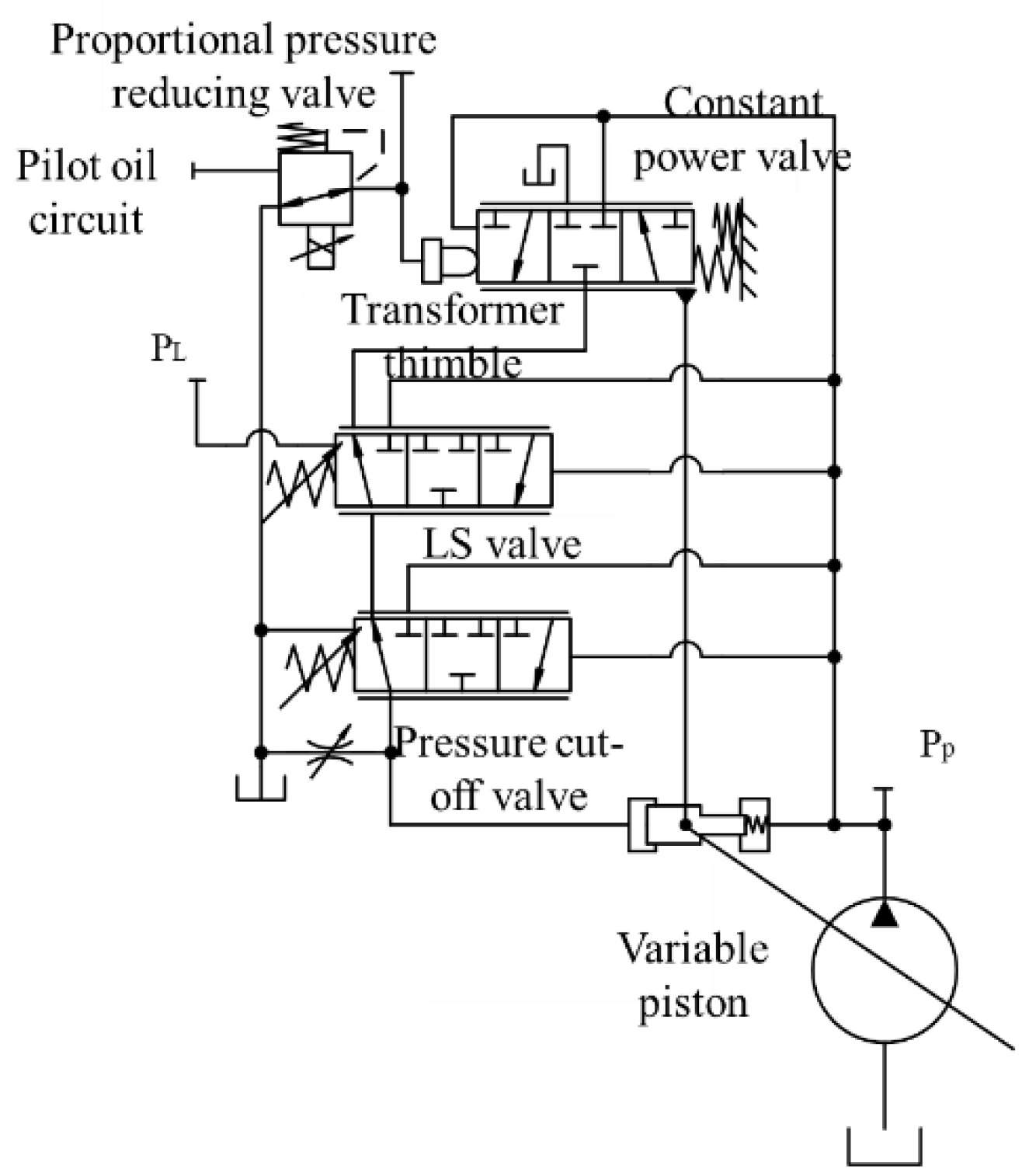
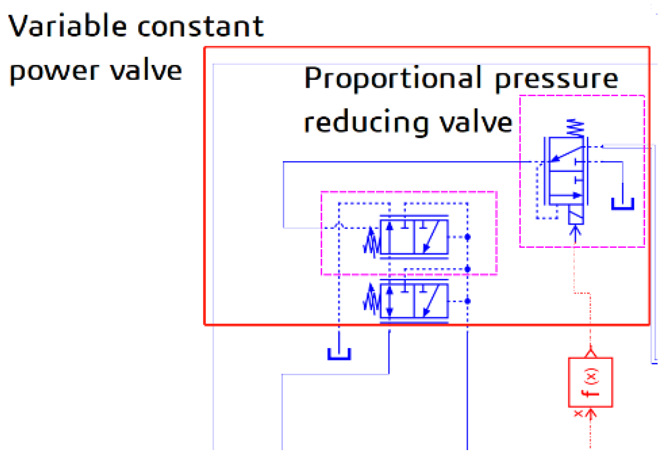
To simplify the simulation model, AMESim module HYDCONLSPC0 is used as the variable constant power valve, as shown in Figure 8. The key parameters of components in the system are given in

Table 2. Parameters of key components.

Speed of Electric Motor	Displacement of Pump	Flow of System	Load Sensing Pressure Difference
500~2000 rpm	8~80 cc/r	4~160 L/min	1.8 MPa

.

5.1. Speed Segmented Flow Control Simulation

For the speed segmented flow control simulation, the action simulation of the single actuator and multi-actuator is carried out to explore the control performance. The upper and lower limits of electric motor speed are set between 500 and 2000 rpm, which is divided into four speed levels: 500 rpm, 1000 rpm, 1500 rpm, and 2000 rpm.

5.1.1. Flow Control Simulation of Single Actuator

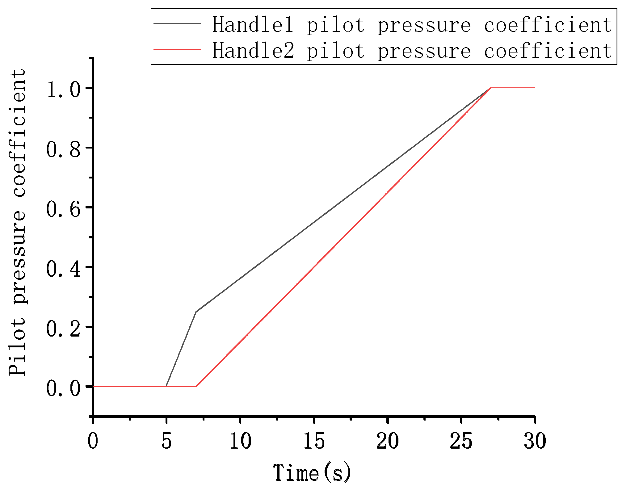
The handle 1 acts alone. Set the maximum flow of the main oil circuit to 160 L/min. Set the pressure of the load proportional overflow valve to 1 MPa. The ratio of target flow to maximum flow is shown in Figure 9.

During 0–5 s, the handle is in the middle position, and ratio of target flow to maximum flow is 0.

During 5–7 s, the ratio of target flow to maximum flow of the handle increases linearly from 0 to 0.25.

During 7–17 s, the ratio of target flow to maximum flow increases linearly from 0.25 to 1.

During 17–22 s, the ratio of target flow to maximum flow remains 1.

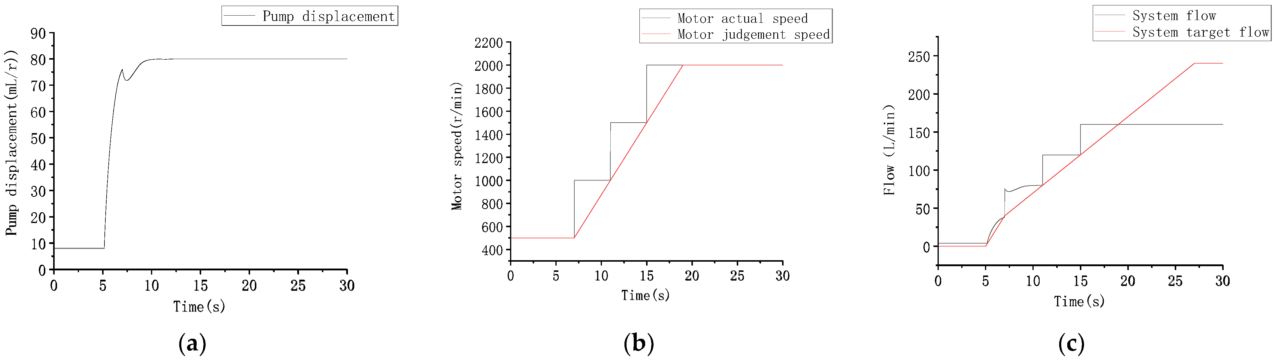
The displacement of variable displacement pump, electric motor speed, and hydraulic system flow can be obtained in Figure 10.

As can be seen, during 0–5 s, the ratio of target flow to the maximum flow of the pilot handle is 0. The target flow of the system is 0 L/min. The electric motor is in the idle stage, and the speed is 500 rpm. The pump works at the minimum displacement of 8 mL/r, so the actual hydraulic system overflows with the minimum flow.

During 5–7 s, the ratio of target flow to the maximum flow of the handle increases from 0 to 0.25. At this time, the target flow of the system increases from 0 to 40 L/min. This stage is in the variable displacement pump stage. The pump displacement increases from 8 to 80 mL/r, which can meet the system flow demand. Therefore, the electric motor keeps running at 500 rpm, the actual flow of the system is 40 L/min, and all flow into the actuator oil circuit.

During 7 to 17 s, the ratio of target flow to maximum flow increases from 0.25 to 1, and the pump displacement remains near the maximum displacement of 80 mL/r. The estimated flow of the system increases with the increase in handle pilot pressure. The electric motor enters the variable speed stage. The system adjusts the electric motor speed step by step according to the speed segmented control strategy. The electric motor speed runs from 500 to 1000 rpm and 1500 to 2000 rpm with the increase in the pilot pressure of the handle. The actual flow of the system also starts from 40 L/min and then at 80 L/min, 120 L/min, and 160 L/min.

During 17 to 22 s, the ratio of target flow to the maximum flow of the handle is maintained at 1. The estimated flow of the system is maintained at 160 L/min. The electric motor is maintained at 2000 rpm. The hydraulic system is maintained at the maximum flow stage.

5.1.2. Flow Control Simulation of Multi-Actuators

Handle 1 controls the maximum flow of the oil circuit at 160 L/min, and handle 2 controls the maximum flow of the oil circuit at 80 L/min. A 1 MPa load is added to oil circuit 1 and oil circuit 2, respectively. To analyze the flow matching of the electric motor-variable speed control system when multiple actuators move and the flow saturation when the target flow is higher than the maximum flow of the system, the multi-actuators flow control simulation of the system is carried out. The input curve of ratios of target flow to a maximum flow of handle 1 and handle 2 is shown in Figure 11.

During 0–5 s, handle 1 and handle 2 remain in the middle position, and the ratios of target flow to maximum flow are 0.

During 5–7 s, the ratio of target flow to the maximum flow of handle 1 increases linearly from 0 to 0.25, and the ratio of target flow to the maximum flow of handle 2 remains 0.

During 7–27 s, the ratio of target flow to the maximum flow of handle 1 increases linearly from 0.25 to 1, and the ratio of target flow to the maximum flow of handle 2 increases from 0 to 1.

During 27 to 30 s, the ratios of target flow to the maximum flow of handle 1 and handle 2 remain 1.

The displacement of the variable displacement pump, electric motor speed, and hydraulic system flow is obtained and given in Figure 12.

During 0–5 s, the ratios of target flow to the maximum flow of handle 1 and handle 2 are 0. The estimated flow of the system is 0 L/min. The electric motor is 500 rpm. The pump is at the minimum displacement of 8 mL/r. Therefore, the actual hydraulic system overflows with a minimum flow of 40 L/min.

During 5–7 s, the ratio of target flow to the maximum flow of handle 1 increases linearly from 0 to 0.25. The ratios of target flow to the maximum flow of handle 2 remain 0. At this time, the estimated flow of the system increases from 0 to 40 L/min. This stage is in the variable displacement stage of the variable displacement pump. The pump displacement increases from 8 to 80 mL/r, which can meet the flow demand of the system. Therefore, the electric motor keeps running at 500 rpm, and the actual flow of the system is 40 L/min, all of which flows into the oil circuit of the actuator.

During 7–19 s, the ratio of target flow to the maximum flow of handle 1 increases linearly from 0.25. The ratio of target flow to the maximum flow of handle 2 increases linearly from 0, and the estimated flow increases linearly from 40 to 160 L/min. The target speed of the electric motor increases from 500 to 2000 rpm. According to the speed segmented control strategy of electric motor speed, the electric motor speed starts from 500 rpm and runs at 1000 rpm, 1500 rpm, and 2000 rpm successively, and the system flow from 40 to 80 L/min, 120 L/min, and 160 L/min successively. The pump displacement shall be kept at the maximum displacement of 80 mL/r.

During 19–27 s, the estimated flow of the system at 19 s reaches the maximum flow of the system, which is 160 L/min. At this time, the motor speed reaches and remains at the maximum speed of 2000 rpm, the variable displacement pump remains at the maximum displacement of 80 mL/r, and the system is in the flow saturation stage. The ratio of target flow to the maximum flow of pilot handle 1 and pilot handle 2 continues to increase linearly to 1, the estimated flow increases linearly to 240 L/min, and the actual system flow remains at 160 L/min.

During 27 to 30 s, the ratios of target flow to the maximum flow of both handles are kept at 1. The pump displacement is kept at the maximum displacement of 80 mL/r. The electric motor speed is kept at the maximum speed of 2000 rpm. The actual system flow is kept at the maximum flow of 160 L/min.

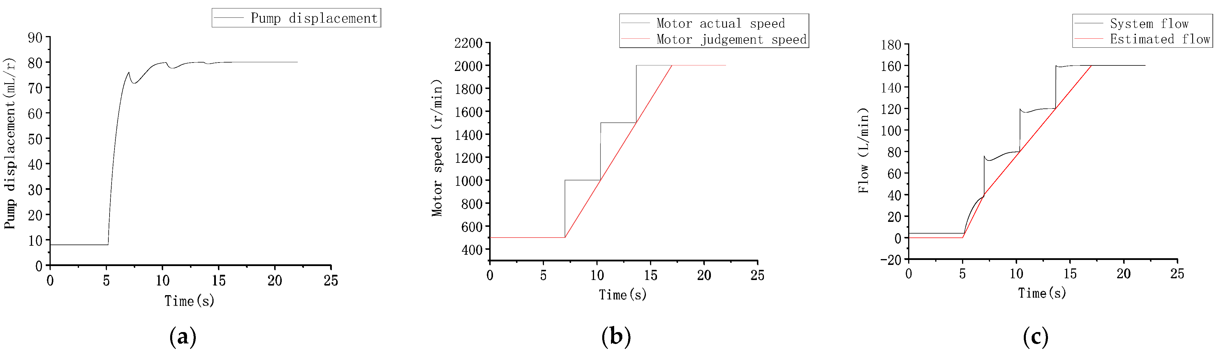
5.2. Speed Segmented Variable Constant Power Control Simulation

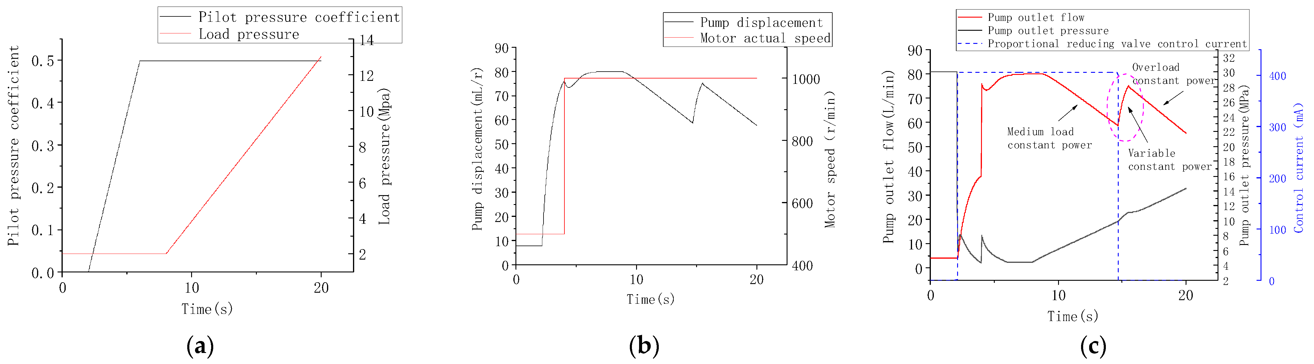
Under the constant power condition, the pump is at a constant speed, and the pump outlet flow changes with the pump outlet pressure. Therefore, the variable constant power control function of the hydraulic pump is realized by making the electric motor at a certain speed level through the speed segmented control strategy. To verify the reliability of the speed segmented variable constant power control system, the electric motor speed stages of 1000 and 2000 rpm are simulated, respectively. The working condition switching is set from medium load to heavy load mode. Set the starting pressure of the medium load constant power valve to 5.1 MPa and that of the heavy load constant power valve to 9.9 MPa. The purpose of this experiment is mainly to verify the function of variable constant power, so the test can be carried out with the movement of a single actuator. The maximum flow of the actuator is 160 L/min. The proportional overflow valve is used to load the oil circuit. The simulation results of test 1 and test 2 are given in Figure 13 and Figure 14, which are the main parameter curves of variable constant power control in the 1000 rpm speed stage and variable power control in the 2000 rpm speed stage, respectively.

As can be seen, the speed segmented control strategy can realize the variable constant power operation in a certain speed range. The time when the two groups of simulation test electric motors reach the fixed speed range is the same. Moreover, the load application is the same. The simulation of variable constant power control under the condition of speed classification is analyzed.

During 0–2 s, the ratio of target flow to the maximum flow of the pilot handle is kept at 0. The pump displacement is the minimum, and the electric motor is kept at an idle speed of 500 rpm. The system is in the minimum flow overflow stage.

During 2–4 s, the ratio of target flow to the maximum flow of the pilot handle increases from 0 to 0.25. The pump displacement increases to 80 mL/r, the motor operates at 500 rpm, the system is in the variable displacement flow control stage, the hydraulic oil flows into the actuator, and the pump outlet pressure decreases.

During 4–6 s, the ratio of target flow to the maximum flow of test I (1000 rpm) and test II (2000 rpm) handle increases from 0.25 to 0.5 and 1, respectively. The pump displacement remains at the maximum value of 80 mL/r. The system is in the variable speed flow control stage. Through the speed segmented control strategy, the system increases to 1000 and 2000 rpm, respectively. The system flow increases to 80 L/min and 160 L/min, respectively.

During 6–9 s, the ratio of target flow to the maximum flow of the handle remains unchanged. Test 1 and test 2 maintain electric motor speed and system flow unchanged; the load gradually increases from 8 s, and the pump outlet pressure also increases. At this time, by monitoring the pump outlet pressure, it is recognized that the working condition is under medium load condition, and the control current of the electric proportional reducing valve is 405 mA.

When the outlet pressure of the pump exceeds the constant load at 15 s, the outlet pressure of the pump increases, and the displacement of the pump decreases.

During 15–20 s, as the load increases, the pump outlet pressure exceeds 9.9 MPa, and the system identifies the working condition as heavy load working condition. The control current of the electric proportional reducing valve changes to 0 mA. The starting regulating pressure of the variable constant power valve changes so that the system works under heavy load working conditions. The pump displacement increases from 58 to 75 mL/ at 15 s so as to realize the adaptive function of working conditions and make the hydraulic pump operate in the heavy load constant power stage. The pump outlet flow continues to decrease as the pump outlet pressure increases.

Based on the above analysis, the speed segmented variable constant power c strategy can enable the hydraulic system to realize the working condition identification at each speed stage and adjust the starting pressure of the variable constant power valve by changing the current of the electric proportional relief valve to realize the working condition adaptation. The simulation results show that the speed segmented variable constant power control is feasible and reliable, which can meet the requirements of variable constant power matching.

6. Experimental Research

Further experimental verification research is carried out. The electric excavator test prototype is built and given in Figure 15. Lithium iron phosphate battery pack and permanent magnet synchronous motor are employed. LUDV system is equipped. The physical drawing and three-dimensional drawing of the system are shown in Figure 16.

By setting the electric motor speed range, the speed segmented strategy is established for the electric motor speed. After calculating the speed according to the target flow, the speed segment standard is obtained for the target speed. According to the allowable speed range of the hydraulic pump used in the experimental platform, the electric motor speed segmented test sets the electric motor speed variation range from 400 to 2400 rpm, and four speed grades are set.

6.1. Test of Single Actuator

A single actuator test takes the boom as an example to monitor the pilot pressure coefficient, boom estimated flow, electric motor judgment speed, motor target speed, and electric motor actual speed. The obtained parameters curves are shown in Figure 17.

The boom single actuator action test completes three lifting and lowering actions by operating the boom pilot hydraulic handle. It can be seen from Figure 17 that the estimated flow of a single actuator changes with the pilot pressure, and the motor judges the speed to follow the estimated flow of the actuator in real time, which ensures the function of predicting the flow and judging the speed to follow the displacement of the hydraulic handle. The whole machine controller determines the speed and speed segmented control strategy by combining the obtained electric motor and giving the target segmented speed. The actual speed of the electric motor actively follows the target speed. It can be seen that the effect of the speed classification strategy is remarkable. The actual speed of the motor strictly follows the speed segmented strategy and has a fast response speed

In Figure 17b, the green circle part shows the obvious embodiment of the speed segmented control strategy. The electric motor judges that the speed fluctuates around 1700 rpm. According to the speed segmented control strategy, the target speed of the motor is set at 2000 rpm, and the actual speed of the motor is also well stable around 2000 rpm, maintaining a small fluctuation range. In this range, the hydraulic pump reduces the displacement through LS pressure to realize the self-adaptive function of pump displacement.

6.2. Test of Multi-Actuators

This takes boom, arm, and bucket pilot hydraulic handles into consideration. Three excavation operations are conducted. The pilot pressure coefficient of each hydraulic handle, the estimated flow of each actuator, the system target flow, the judgment speed of the motor, the target speed of the motor, and the actual speed of the motor are shown in Figure 18.

The circled part in Figure 18b is in a flow saturation state. The electric motor operates at the maximum speed of 2400 rpm. In Figure 18c, the actual speed of the electric motor can follow the target speed of the electric motor in time. When it is in the flow saturation stage, the electric motor operates at the maximum speed. When the electric motor judges that the speed is lower than 400 rpm, both the target speed and the actual speed of the motor operate at 400 rpm. Figure 18d is a partially enlarged view of area A in Figure 18c, recording the curve between the judged speed of the motor, the target speed of the electric motor, and the actual speed of the electric motor during 6.5–12.5 s, which can verify that the motor speed segmented strategy has superior reliability and fast response ability.

6.3. Electric Motor Speed Segmented Variable Constant Power Control Strategy Test

By monitoring the pump outlet pressure, the current working condition of the electric excavator is automatically identified. The pump outlet pressure is related to the maximum load of the actuator, so the relevant parameters are analyzed by a single actuator action test. Because the pump outlet pressure fluctuates greatly, the pump outlet pressure needs to be filtered, and the threshold filtering method is adopted. The pump outlet pressure and the pump outlet pressure after filtering are given in Figure 19. The estimated curves of electric motor speed and flow are given in Figure 20.

As can be seen in Figure 19, threshold filtering can effectively filter out the fluctuation of pump outlet pressure, and a relatively smooth pump outlet pressure curve can be obtained. A superior follow-up effect on the actual pump outlet pressure curve can be obtained as well. Through the condition adaptive control strategy, the control current I curve of the input electric proportional relief valve is obtained so as to adjust the starting pressure of the constant power valve and realize the condition adaptive function of the hydraulic pump. From the curve of electric motor speed and estimated flow in Figure 20, using the control strategy of electric motor segmented speed can get a better effect.

7. Conclusions

Electric construction machinery is considered to be one of the main trends in the future. However, most of the existing electric construction machinery has not yet considered the matching control between the electric motor and hydraulic pump.

In this paper, an electric excavator is taken for study. Based on the LUDV system of construction machinery, a control strategy based on motor speed classification and variable constant power can automatically identify the actual working conditions of the electric excavator and adjust the starting pressure of the constant power valve, to change the constant power range of hydraulic pump and achieve the goal of adapting to the working conditions of power system, is proposed. Simulation and experiments are carried out to verify the feasibility of the proposed control strategy. The results show that the speed classification and variable constant power control system can effectively realize the segmented regulation of motor speed and provide relatively stable speed input for the hydraulic system. Moreover, the current working condition can be identified through the pump outlet pressure. The adaption of working conditions can be realized through the proportional reducing valve by adjusting the starting pressure of the variable constant power valve.

In this paper, the external characteristics of the motor pump have been studied, but the internal characteristics of the motor pump have not been studied. Further research will be carried out later.

References

1. Wargua, U.; Lijewski, P.; Kukla, M. Influence of non-commercial fuel supply systems on small engine SI exhaust emissions in relation to European approval regulations. Environ. Sci. Pollut. Res. 2022, 29, 55928–55943. [Google Scholar] [CrossRef] [PubMed]
2. Domeika, R. Analysis of Telematics Data of Combine Harvesters and Evaluation of Potential to Reduce Environmental Pollution. Atmosphere 2021, 12, 674. [Google Scholar] [CrossRef]
3. Tu, R.; Li, T.; Meng, C.; Chen, J.; Sheng, Z.; Xie, Y.; Xie, F.; Yang, F.; Chen, H.; Li, Y.; et al. Real-world Emissions of Construction Mobile Machines and Comparison to a Non-road Emission Model. Sci. Total Environ. 2021, 771, 145365. [Google Scholar] [CrossRef] [PubMed]
4. Kagoshima, M.; Komiyama, M.; Nanjo, T.; Tsutsui, A. Development of new hybrid excavator. Kobelco Technol. Rev. 2007, 27, 39–42. [Google Scholar]
5. Chen, Q.; Lin, T.; Ren, H.; Fu, S. Novel potential energy regeneration systems for hybrid hydraulic excavators. Math. Comput. Simul. 2019, 163, 130–145. [Google Scholar] [CrossRef]
6. Yu, Y.; Ahn, K. Energy Saving of an Electric Forklift with Hydraulic Accumulator. In Proceedings of the 19th International Conference on Control, Automation and Systems, Jeju, Korea, 15–18 October 2019. [Google Scholar]
7. Lin, T. Energy-Saving Technology and Application of Construction Machinery; China Machine Press: Beijing, China, 2018. [Google Scholar]
8. Gao, F.; Wang, S.; Gao, J. Automatic control method research on pendulum speed of roadheader’s cutting arm. In Proceedings of the 2011 Second International Conference on Mechanic Automation and Control Engineering, Hohhot, China, 15–17 July 2011; pp. 4789–4791. [Google Scholar]
9. Ren, H.; Lin, T.; Zhou, S.; Huang, W.; Miao, C. Novel Automatic Idle Speed Control System with Hydraulic Accumulator and Control Strategy for Construction Machinery. Appl. Sci. 2018, 8, 496. [Google Scholar] [CrossRef]
10. Chen, Z.; Sun, Z. Using variable piston trajectory to reduce engine-out emissions. Appl. Energy 2016, 170, 403–414. [Google Scholar]
11. Zsiga, N.; Ritzmann, J.; Soltic, P. Practical Aspects of Cylinder Deactivation and Reactivation. Energies 2021, 14, 2540. [Google Scholar] [CrossRef]
12. Wen, Q.; Wang, F.; Xu, B.; Sun, Z. Improving the Fuel Efficiency of Compact Wheel Loader with a Series Hydraulic Hybrid Powertrain. IEEE Trans. Veh. Technol. 2020, 69, 10700–10709. [Google Scholar] [CrossRef]
13. Li, P.Y.; Siefert, J.; Bigelow, D. A Hybrid Hydraulic-Electric Architecture (HHEA) for High Power Off-Road Mobile Machines. In Proceedings of the ASME FPMC 2019, Sarasota, FL, USA, 7–9 October 2019. [Google Scholar]
14. Chen, Q.; Lin, T.; Ren, H. Parameters optimization and control strategy of power train systems in hybrid hydraulic excavators. Mechatronics 2018, 56, 16–25. [Google Scholar] [CrossRef]
15. Lin, T.; Chen, Q.; Fu, S. Key Technology and Application of Electric Excavator; China Machine Press: Beijing, China, 2018. [Google Scholar]
16. Lin, T.; Lin, Y.; Ren, H.; Chen, H.; Chen, Q.; Li, Z. Development and key technologies of pure electric construction machinery. Renew. Sustain. Energy Rev. 2020, 132, 110080. [Google Scholar] [CrossRef]
17. Ge, L.; Quan, L.; Zhang, X.; Zhao, B.; Yang, J. Efficiency Improvement and Evaluation of Electric Hydraulic Excavator with Speed and Displacement Variable Pump. Energy Convers. Manag. 2017, 150, 62–71. [Google Scholar] [CrossRef]
18. Liu, B.; Quan, L.; Ge, L. Research on Energy Consumption Characteristics of Variable Speed and Variable Displacement Electric Drive Hydraulic Excavator. Chin. Hydraul. Pneum. 2020, 37, 7–13. [Google Scholar]
19. Lin, T.; Huang, W.P.; Ren, H.; Fu, S.; Chen, Q.; Liu, Q. Automatic Idle Speed Control of Load Sensing for Electric-Driven Construction Machinery. J. Shanghai Jiaotong Univ. 2016, 50, 1929–1935. [Google Scholar]
20. Lin, T.; Wang, L.; Huang, W.; Ren, H.; Fu, S.; Chen, Q. Performance Analysis of an Automatic Idle Speed Control System with a Hydraulic Accumulator for Pure Electric Construction Machinery. Autom. Constr. 2017, 84, 184–194. [Google Scholar] [CrossRef]
21. Yoon, J.I.; Truong, D.Q.; Ahn, K.K. A Generation Step for an Electric Excavator with a Control Strategy and Verifications of Energy Consumption. Int. J. Precis. Eng. Manuf. 2013, 14, 755–766. [Google Scholar] [CrossRef]
22. Zhang, S.; Minav, T.; Pietola, M. Improving Efficiency of Micro Excavator with Decentralized Hydraulics. In Proceedings of the ASME/BATH 2017 Symposium on Fluid Power and Motion Control, Sarasota, FL, USA, 16–19 October 2017; American Society of Mechanical Engineers Digital Collection: New York, NY, USA, 2017. [Google Scholar]
Figure 1. Structural principle diagram of constant power regulation system.
Applsci 12 09734 g001
Figure 2. Outlet pressure variation with flow curve of constant power pump.
Applsci 12 09734 g002
Figure 3. Internal schematic diagram of load sensing pump.
Applsci 12 09734 g003
Figure 4. Constant power curve under different working conditions.
Applsci 12 09734 g004
Figure 5. Schematic diagram of speed segmented variable constant power control.
Applsci 12 09734 g005
Figure 6. Schematic diagram of speed segmented variable constant power control.
Applsci 12 09734 g006
Figure 7. Simulation model in AMESim.
Applsci 12 09734 g007
Figure 8. Variable constant power module in the simulation model.
Applsci 12 09734 g008
Figure 9. Pilot signal curve.
Applsci 12 09734 g009
Figure 10. Pump displacement, motor speed, and system flow curve. (a) Curve of pump displacement; (b) curve of electric motor speed; (c) curve of system flow.
Applsci 12 09734 g010
Figure 11. Multi-handles input signal.
Applsci 12 09734 g011
Figure 12. Pump displacement, electric motor speed, and system flow curve. (a) Curve of pump displacement; (b) curve of electric motor speed; (c) curve of system flow.
Applsci 12 09734 g012
Figure 13. Simulation curve of variable constant power control of electric motor at 1000 rpm. (a) Curve of handle signal and load; (b) curve of pump displacement and electric motor speed; (c) curve of outlet flow and pressure of the pump and current of electro proportional reducing valve.
Applsci 12 09734 g013
Figure 14. Simulation curve of variable constant power control of electric motor at 2000 rpm. (a) Curve of handle signal and load; (b) curve of pump displacement and electric motor speed; (c) curve of outlet flow and pressure of the pump and current of electro proportional reducing valve.
Applsci 12 09734 g014
Figure 15. System structure diagram of electric excavator test prototype.
Applsci 12 09734 g015
Figure 16. Physical drawing and three-dimensional drawing of part of the system.
Applsci 12 09734 g016
Figure 17. Relevant parameter curves of electric motor speed segmented control. (a) Pilot signal and estimated flow curve of the system; (b) electric motor judgment speed, motor target speed, and motor actual speed curve.
Applsci 12 09734 g017
Figure 18. Curves of electric motor speed segmented control for the multi-actuator test. (a) Pilot signal of each actuator; (b) estimated flow of each actuator; (c) electric motor speed; (d) partial enlarged view of part A in Figure 18c.
Applsci 12 09734 g018
Figure 19. Curves of pump outlet pressure and control current of electro proportional reducing valve.
Applsci 12 09734 g019
Figure 20. Curves of electric motor speed and estimated flow of the system.
Applsci 12 09734 g020