Aerodynamic Modeling and Performance Analysis of Variable-Speed Coaxial Helicopter

Abstract

In this paper, the variable-speed coaxial helicopter is modelled by the blade element method, non-uniform inflow method and empirical function method, and the aerodynamic performance analysis method is proposed. To ensure the accuracy of this method, a flight test of the verification aircraft has been performed, and the rotor speed and required power under different forward flight speeds have been obtained. By comparing the experimental results with the calculation results, it is ascertained that the rotor speed trim error of this method is less than 6%, and the required power calculation error is less than 5%, which demonstrates the accuracy of this method. Finally, when the rotor diameter, hovering collective pitch and hovering rotor speed are equal, the required power of variable-speed coaxial helicopter and variable collective-pitch coaxial helicopter is compared through this method. The comparison results show that the variable-speed coaxial helicopter has low required power when it is less than the forward flight speed corresponding to the hovering rotor speed. When the forward speed is higher than that corresponding to the hovering rotor speed, the variable-pitch coaxial helicopter has lower required power.

1. Introduction

In recent years, with the development of motor and speed control technology, the control of variable-speed aircraft such as multi-rotor aircraft has been evolving with more possibilities at low speed. The study has extensive applications in both the military and civil aircraft industry over conventional single rotor aircraft. This makes the variable-speed rotor aircraft a topic of concern for researchers across the globe. However, the traditional helicopter can fly at high speed, and there is a potential for its miniaturization and lightweight. This requires the integration of the earlier two to obtain a small variable-speed helicopter with lighter structure weight, better reliability and higher flight efficiency. The coaxial rotor produces a counterrotating torque which cancels out the need for an additional tail rotor, thereby reducing the weight and power consumed by the tail rotor. A study on a rigid coaxial blade based on the principle of the Advanced Blade concept (ABC) in support of the Sikorsky ABC helicopter program revealed an improved forward flight performance and reduced excessive tip deflections and extreme moments, thereby utilizing the maximum ability of the blade for generating lift [1]. There are limited studies on the aerodynamics of multirotor aircraft; however, the earliest research survey [2] carried out for multirotor aerodynamics revealed a positive insight into coaxial rotor in hover, since it has no tail rotor, along with the minimum power requirement when compared to conventional single axis rotor, and the forward flight performance revealed a lower power requirement for moderate advance ratios contradicting with high drag penalty for higher advance ratios.

In 2012, Xia Qingyuan and Xu Jin applied the blade element momentum theory (BEMT) method to calculate the load of variable-speed coaxial rotor, and they verified it through experiments [3]. A formal optimization model of coaxial rotor for helicopters operating in hover and the axial forward flight was studied by [4], which showed a better prediction of results when compared to the simple momentum theory. However, the BEMT method has a range of deficiencies, such as unclear physical meaning, which may lead to deviation of the results. Further, the coaxial rotor wake dynamics, wake structure and ground effects were optimized using the free-vortex filament method for maneuvering flight conditions [5,6,7]. The study by [8] studied the free Lagrangian Incompressible Navier–Stokes Equation. The full-scale wind tunnel experimental investigations were performed by [9], calculating the static thrust performance of both coaxial and single-axis rotor blades tapered in both planform and thickness ratio. This is followed by the study performed on a coaxial-configured-rotor and tandem-rotor arrangement, revealing an increase in hovering efficiency for tandem rotors spaced exactly one rotor diameter apart. The power requirement identifies with the previously available theories. The hover performance of single, coaxial, tandem and tiltrotor configurations was investigated by [10], briefing about the interference losses and rotor-on-rotor effect. A high-speed steady-level forward flight was simulated using CFD–CSD coupling correlated to the vortex wake model by [11], who stated the rotor interference was found to agree with the momentum theory and captured the cross transition of flow across the rotor blades, thereby quantifying the effects of pitching moment, which shows negligible torsional response on the rotor. While understanding the coaxial rotor system, trim becomes one of the important parameters, since the torque should be balanced between hover and forward flight, with the respective lift offset by providing proper controls. A 3D numerical simulation with overlapped grid on a rotor in forwarding flight conditions was analyzed by [12]. This is based on Euler and Navier–Stokes Equation and was later found to be in line with the flight test data. In 2017, Zhao Qibing and Liu Yong of Nanjing studied the controllability of variable-range multi-rotor aircraft and pointed out the change in controllability after several rotor failures [13]. In 2018, Song Yanguo, Wang huanjin and others from the Nanjing University of Aeronautics and Astronautics applied the unsteady model to analyze the performance of variable-pitch multi-rotor aircraft and conducted experimental verification [14], and obtained highly reliable results. In 2020, the New Rotor Aircraft Laboratory of the Aviation Industry Helicopter Institute launched a variable-range multi-rotor aircraft, AR20, which has excellent aerodynamic performance. In 2007, M López-Martínez et al. used Proportional Integral Derivative (PID) control law to study the nonlinear control of a variable-speed twin rotor and carried out experimental verification [15]. In 2016, Lidia et al. studied the decentralized Active Disturbance Rejection Control (ADRC) speed control of the rotor in the laboratory, which simplified the controller design task and improved the robustness of the control [16]. The Helicopter Research Institute of Beihang University has also studied this kind of aircraft and designed a variable-speed coaxial helicopter, D-07, which stands out for its high efficiency and portability.

Even though various researchers performed their research on variable-speed coaxial rotor aerodynamics, the approach contains various performance parameters using mathematical formulation, and its verification through experiment is still a gap. This paper will describe the aerodynamic performance analysis method of a variable-speed coaxial helicopter, and it will verify the feasibility of this method through actual flight tests. Finally, the authors also compare the required power of variable-pitch coaxial helicopters and variable-speed coaxial helicopters and analyze the reasons for the differences between them.

2. Establishment of an Aerodynamic Model

2.1. Rotor Aerodynamic Model

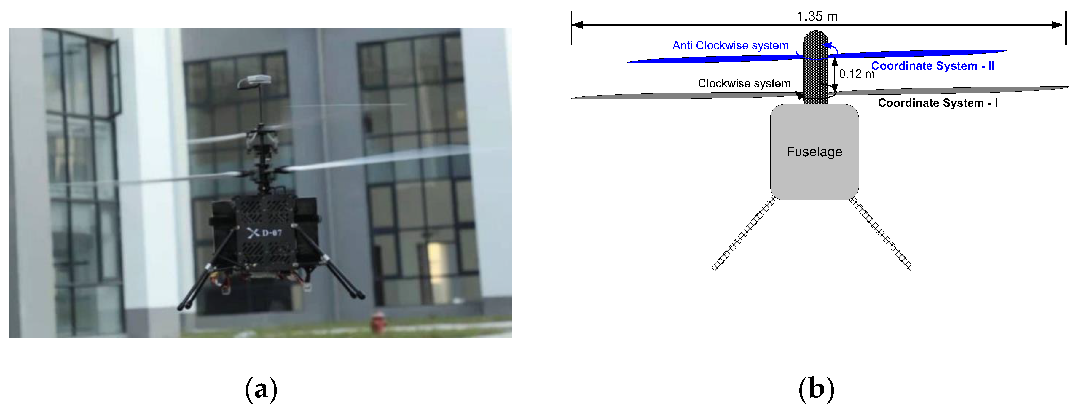
2.1.1. Definition of the Coordinate System

Due to the opposite rotation of the coaxial rotors, the rotor and hub coordinate systems of the lower rotor are assumed to be based on the right-hand system, whereas the rotor and hub coordinate systems of the upper rotor are assumed based on the left-hand system. Therefore, the lower rotor is designated with the coordinate system I, and the upper rotor is designated with coordinate system II. The rotor coordinate system is a transitional coordinate system, which is convenient to calculate the rotor aerodynamic force. The origin of the hub coordinate system is defined at the center of the hub. The origin of the fuselage coordinate system is located at the center of gravity of the fuselage and is in the right-hand system.

The rotor aerodynamic force calculated by the blade element method is in the rotor coordinate system and needs to be converted into the hub coordinate system. Taking the following rotor as an example, the conversion relationship is:

$$\begin{gathered} \left[\begin{array}{c}{X}_{H1}\\ Y_{H1}\\ Z_{H1}\end{array}\right]=\left[\begin{array}{c}-H_1\\ Y_1\\ -T_1\end{array}\right] \\ \left[\begin{array}{c}{L}_{H1}\\ M_{H1}\\ N_{H1}\end{array}\right]=\left[\begin{array}{c}-L_1\\ M_1\\ -N_1\end{array}\right] \end{gathered}$$

(1)

From the equation, H₁ is the backward force of the lower rotor, Y₁ is the lateral force of the lower rotor, T₁ is the pull force of the lower rotor, L₁ is the roll moment of the lower rotor, M₁ is the pitch moment of the lower rotor, N₁ is the yaw moment of the lower rotor, X_H1, Y_H1 and Z_H1 are the three-dimensional forces of the lower rotor in the hub coordinate system, and L_H1, M_H1 and N_H1 are the three-dimensional moments of the lower rotor around the X, Y and Z axes in the hub coordinate system. The expressions of the forces and moments of the upper rotor are the same as those of the lower rotor, and only the footmark needs to be changed.

The balanced equation below is established in the body coordinate system, so it will involve the mutual transformation of the left- and right-hand systems. The transformation relationship is as follows:

$$\begin{gathered} {\left[\begin{array}{c}{X}_{H2}\\ Y_{H2}\\ Z_{H2}\end{array}\right]}_{LEFT}\Rightarrow {\left[\begin{array}{c}{X}_{H2}\\ -Y_{H2}\\ Z_{H2}\end{array}\right]}_{RIGHT} \\ {\left[\begin{array}{c}{L}_{H2}\\ M_{H2}\\ N_{H2}\end{array}\right]}_{LEFT}\Rightarrow {\left[\begin{array}{c}-L_{H2}\\ M_{H2}\\ -N_{H2}\end{array}\right]}_{RIGHT} \end{gathered}$$

(2)

X_H2, Y_H2, Z_H2 are the three-dimensional forces of the upper rotor in the hub coordinate system, and L_H2, M_H2 and N_H2 are the three-dimensional moments of the upper rotor around the X, Y and Z axes in the hub coordinate system. For the left- and right-hand systems, the x-axis points to the forward flight direction.

2.1.2. Rotor Aerodynamic Force

In this paper, the blade element method will be used to model the aerodynamic forces of the upper and lower rotors, but the expression variables derived from the original blade element method include the total pitch angle. However, the total pitch angle of the coaxial unmanned helicopter in this paper remains unchanged, and the speed changes. Therefore, the dimensionless blade element theoretical expression should be transformed into the blade element theoretical expression whose variable is the speed.

Through the blade element theory, the forces and moments of the upper and lower rotors in the rotor coordinate system can be deduced. Due to the complexity of the final expressions of these forces and moments, only the more characteristic expressions of lower rotor tension are described, and the expressions of other forces and moments can be obtained one by one by this method. The pull force of the lower rotor can be expressed as [17]:

$$\begin{array}{l}{T}_1=\frac{1}{4}{N}_b\rho ac{\Omega }^2{R}^3\left\{\right({\theta }_0+{\theta }_{01})\left(\frac{2}{3}+{\mu }_1{}^2-\epsilon {\mu }_1{}^2\right)\\ +{\theta }_t[\frac{1}{2}-\frac{2}{3}\epsilon +\frac{1}{2}{\mu }_1{}^2\left(1-{\epsilon }^2\right)]\\ -B_1{\mu }_1\left(1-{\epsilon }^2\right)+{\lambda }_1\left(1-{\epsilon }^2\right)+a_1\epsilon {\mu }_1\left(1-\epsilon \right)\}\end{array}$$

(3)

where N_b is the number of blades, ρ is the air density, a is the lift line slope, c is the blade chord length, Ω is the rotor speed, ${\theta }_0$ is the blade installation angle, ${\theta }_{01}$ is the heading differential angle of the lower rotor, ${\theta }_t$ is the blade torsion angle, ε is the dimensionless swing hinge offset, ${\mu }_1$ is the forward ratio of the lower rotor, ${\lambda }_1$ is the inflow ratio of the lower rotor, B₁ is the longitudinal periodic pitch of the upper and lower rotors, and a₁ is the rear chamfer of the lower rotor.

In the expressions of all forces and moments, the inflow ratio and forward ratio are with speed variables. The inflow ratio and forward ratio can be expressed as:

$$\begin{array}{c}{\mu }_1=\frac{\sqrt{V_x^2+V_y^2}}{\Omega R}\end{array}$$

(4)

$$\begin{array}{c}{\lambda }_1=\frac{V_z-\left(v_1+{\delta }_1{v}_2\right)}{\Omega R}\end{array}$$

(5)

where v₁ and v₂ are the induced velocities of the lower and upper rotors, respectively, and V_X, V_Y and V_Z are the components of the incoming flow along each axis of the rotor coordinate system. ${\delta }_1$ is the interference coefficient between the upper rotor and the lower rotor. See the induced velocity model for the specific calculation method.

2.2. Induced Velocity Model

The induced velocity model in this paper adopts the static non-uniform inflow calculation model of the coaxial rotor in the form of a first-order harmonic [18]. To consider the interference of upper and lower rotors, the rotor interference coefficient is introduced. The hovering interference model adopts the upper and lower rotor interference model [19] obtained by McAlister and other scholars according to the experimental data and the numerical simulation of the Biot Savart theorem, which can be expressed as:

$$\begin{array}{c}\delta =1+{\left(\frac{|\overline{z}|}{\sqrt{1+{\overline{z}}^2}}\right)}^{k}sign\left(\overline{z}\right)\end{array}$$

(6)

From the equation, δ is the interference coefficient of the upper and lower rotors, z is the vertical distance between the analysis rotor and the rotor generated by the interference, and constant k is the empirical coefficient. When analyzing the interference of the lower rotor to the upper rotor, k is taken as 0.6, and when analyzing the interference of the upper rotor to the lower rotor, K is taken as 0.3–0.5. During forward flight, the empirical functions [20] K₁ and K₂ of the wake inclination of the lower and upper rotors are introduced, respectively, where the expression of K₁ is:

$$\begin{array}{c}{K}_1=\frac{15\pi }{32}\mathit{tan}\left(\frac{{\chi }_1}{2}\right)\end{array}$$

(7)

From the equation, ${\chi }_1$ is the inclination angle of the wake, which can be expressed as:

$$\begin{array}{c}{\chi }_1={\mathit{tan}}^{-1}\left(\frac{{\mu }_1}{-{\lambda }_1}\right)\end{array}$$

(8)

After considering the above interference model, the induced velocity model of the lower rotor can be expressed as:

$$\begin{array}{c}{v}_{1,total}=v_1+{\delta }_1{v}_2\left(K_1{v}_1+K_2{\delta }_1{v}_2\right)\frac{r}{R}\mathit{cos}\left({\psi }_1\right)\end{array}$$

(9)

From the equation, ${\psi }_1$ is the blade azimuth.

2.3. Dynamic Model of Blade Swing

Taking the following rotor swing as an example, the swing motion equation [21] of the blade can be obtained from the balance of various moments at the swing hinge:

$$\begin{array}{c}{I}_{\beta }\ddot{\beta }+I_{\beta }{\Omega }^2\beta +M_C+M_R=M_T-M_{S}g\end{array}$$

(10)

where $I_{\beta }$ is the moment of inertia of the blade around the swing hinge, β is the swing angle, M_C is the Coriolis moment, M_R is the restraint moment of the swing hinge, M_T is the aerodynamic moment, and M_S is the mass static moment of the rotor around the swing hinge. For rectangular blades, $I_{\beta }$ can be expressed as:

$$\begin{array}{c}{I}_{\beta }=m{x}^2\end{array}$$

(11)

where m is the mass of the blade and x is the distance from the center of gravity of the blade to the rotation axis. For rectangular blades, M_S can be expressed as:

$$\begin{array}{c}{M}_S=mx\end{array}$$

(12)

For rotors with swing angle constraints, M_R can be expressed as:

$$\begin{array}{c}{M}_R=K\beta \end{array}$$

(13)

where K is the stiffness coefficient of flapping rubber, in N·m/rad. The aerodynamic moment M_T can be obtained by integrating the blade element theory. After sorting, the blade flapping motion equation can be obtained:

$$\left[\begin{array}{c}\ddot{a_0}\\ \ddot{a_1}\\ \ddot{b_1}\end{array}\right]+D\left[\begin{array}{c}\dot{a_0}\\ \dot{a_1}\\ \dot{b_1}\end{array}\right]+K\left[\begin{array}{c}{a}_0\\ a_1\\ b_1\end{array}\right]=f$$

(14)

where f can be expressed as:

$$f=F_1\left[\begin{array}{c}{\theta }_0\\ {\theta }_t\\ A_1\\ B_1\end{array}\right]+F_2\left[\begin{array}{c}{\omega }_x\\ {\omega }_z\end{array}\right]+F_3{\lambda }_1+F_4$$

(15)

Among them, D, K, F₁, F₂, F₃ and F₄ are coefficient matrices and vectors, and their values are related to the swing hinge offset, swing rubber stiffness, incoming flow condition and blade lock number of the rotor. It is worth mentioning that after derivation, F₄ is related to various inertia forces and moments of the blade, and attention should be paid to the position of the speed variable; otherwise, the final equation group will have no solution, and its specific expression is:

$$\begin{array}{c}{F}_4=\left[\begin{array}{c}-\frac{M_s}{I_{\beta }{\Omega }^2}g\\ \frac{\gamma }{2}\left(\frac{K_1{v}_1+K_2{\delta }_1{v}_2}{\Omega R}\right)\left(\frac{1}{4}-\frac{2}{3}\epsilon +\frac{1}{2}{\epsilon }^2\right)\\ 0\end{array}\right]\end{array}$$

(16)

where G is the acceleration of gravity, and γ is the number of blades.

3. Model Solution and Experimental Verification

3.1. Verification Machine D-07

In this paper, the D-07 variable-speed coaxial helicopter developed by the Helicopter Research Institute of Beihang University is used as the verification aircraft. The main purpose of this aircraft is to break through the flight time of an electric helicopter. Its main characteristics are as follows:

(1)

A new type of coaxial helicopter control mechanism is proposed, which adopts the control strategy of fixed pitch and variable speed, which greatly reduces the weight of the control system.

(2)

A coaxial helicopter transmission system is proposed, which adopts new materials and optimizes the processing mode to make its empty weight meet the requirements.

(3)

According to the dynamic analysis, the model of the aircraft is designed, and the problem of strong vertical head coupling is solved. The parameters of D-07 are shown in

Table 1. D-07 parameters.

Parameter	Numerical Value
Rotor diameter	1.35 m
Number of rotors	2
Rotor mounting angle	12°
Maximum takeoff weight	7 kg
Battery capacity	16 Ah
Swing hinge offset	0.011 m
Distance between upper and lower rotors	0.12 m
Flapping rubber stiffness coefficient	288 N·m/rad
Blade weight	150 g
Lower rotor coordinates (under fuselage coordinate system)	(0, 0, 0.13)
Rotor coordinates (under fuselage coordinate system)	(0, 0, 0.25)

. The actual outline drawing of D-07 is shown in Figure 1.

3.2. Model Solution

According to the above model analysis and further substituting various parameters of D-07, a nonlinear equation can be obtained, which can be expressed as:

$$\begin{gathered} \left[\begin{array}{c}{X}_{H1}+X_{H2}\\ Y_{H1}+Y_{H2}\\ Z_{H1}+Z_{H2}\\ (L_{H1}+y_1{Z}_{H1}-z_1{Y}_{H1})+(L_{H2}+y_2{Z}_{H2}-z_2{Y}_{H2})\\ (M_{H1}+z_1{X}_{H1}-x_1{Z}_{H1})+(M_{H2}+z_2{X}_{H2}-x_2{Z}_{H2})\\ (N_{H1}+x_1{Y}_{H1}-y_1{X}_{H1})+(N_{H2}+x_2{Y}_{H2}-y_2{X}_{H2})\end{array}\right]=\left[\begin{array}{c}{m}_{total}g\mathit{sin}\left(\theta \right)+F_{drag,x}\\ -m_{total}gcos\left(\theta \right)\mathit{sin}\left(\phi \right)+F_{drag,y}\\ -m_{total}g\mathit{cos}\left(\theta \right)\mathit{cos}\left(\phi \right)+F_{drag,z}\\ F_{drag,L}\\ F_{drag,M}\\ F_{drag,N}\end{array}\right] \\ {K}_1\left[\begin{array}{c}{a}_{01}\\ a_{11}\\ b_{11}\end{array}\right]=f_1 \\ {K}_2\left[\begin{array}{c}{a}_{02}\\ a_{12}\\ b_{12}\end{array}\right]=f_2 \\ {\left[\begin{array}{c}{T}_1\\ T_2\end{array}\right]}_{Leaf element}={\left[\begin{array}{c}{T}_1\\ T_2\end{array}\right]}_{Slipstream} \end{gathered}$$

(17)

where x, y and z are the coordinate values of the upper and lower rotor hubs in the fuselage coordinate system, F drag is the fuselage drag and T is the torque, and the two sides of the last two equations are the tension calculated by the blade element method and the momentum method, respectively, in which the empirical parameters such as blade tip loss are taken into account. It should be noted that all forces and moments in the above nonlinear equations are established in the fuselage coordinate system. The equations contain 14 variables, including the induced speeds V₁ and V₂ of the lower and upper rotors, the swing angles a₀₁, a₀₂, a₁₁, a₁₂, b₁₁ and b₁₂ of the lower and upper rotors, the periodic variable distances A1 and B1 of the upper and lower rotors, and the course control θ₀₁, upper and lower rotor speed Ω, fuselage pitch angle θ, Fuselage roll angle φ, So the equations are closed.

As it is a nonlinear equation, Newton Raphson’s method is used to solve it in this paper. The solving step is to first calculate the Jacobian matrix of the nonlinear equations, and then iteratively solve it through Newton’s iterative formula to obtain the state vector of the coaxial helicopter after balancing. Newton’s iterative formula, used for the calculation, is represented by Equation (18):

$$\begin{array}{c}{x}_{n+1}=x_n-\frac{f\left(x_n\right)}{f^{\prime }\left(x_n\right)}\end{array}$$

(18)

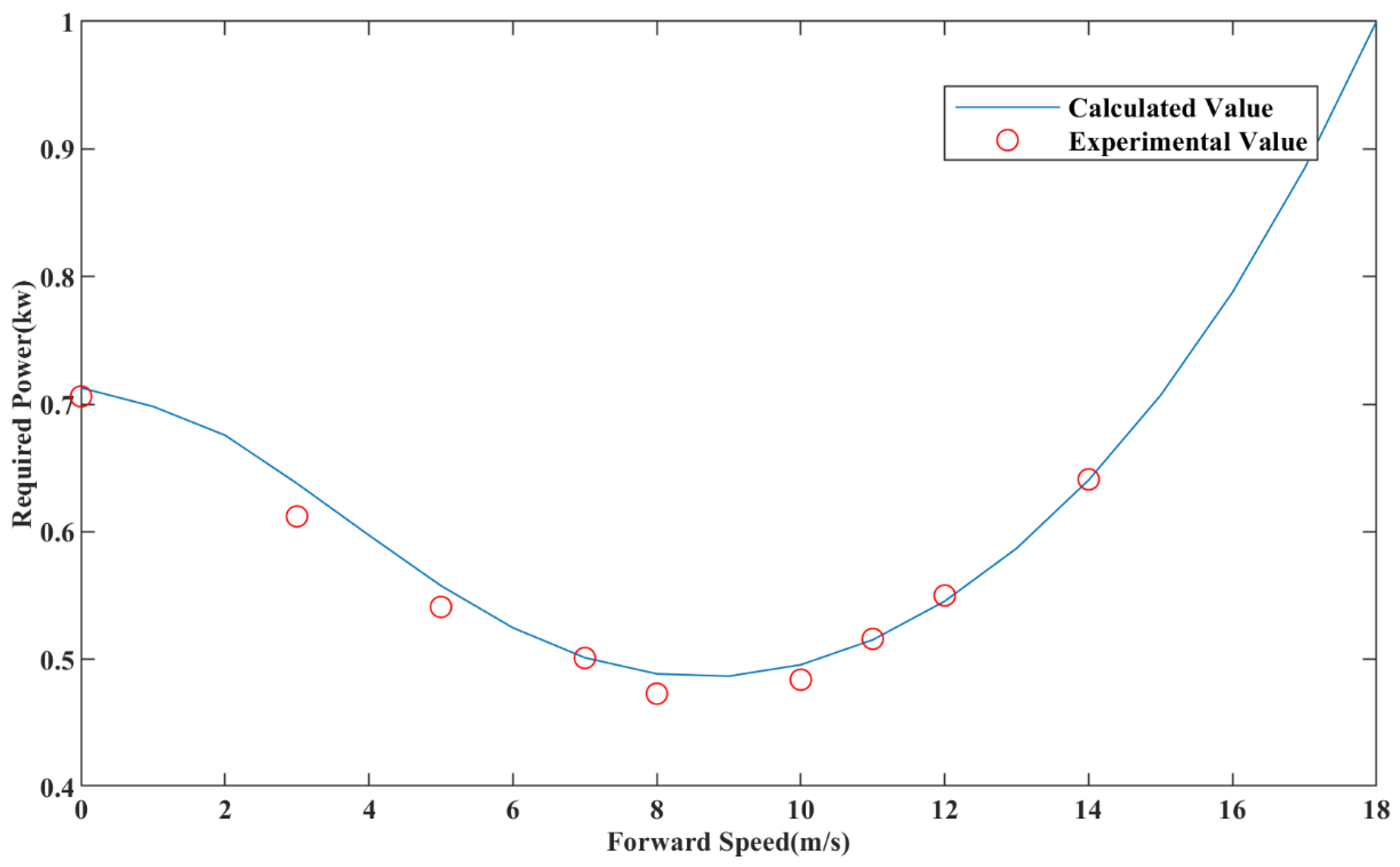
3.3. Calculation Results and Experimental Verification

To verify the accuracy of the calculated results, the flight test of the verification aircraft is carried out, and the data is presented in this paper. The comparison between the rotor speed of trim and the actual rotor speed of the verification aircraft under different forward flight speeds is obtained, as shown in Figure 2. With the increase in forwarding flight speed, the rotor speed curve presents a saddle shape.

It can be seen from Figure 2 that the difference between the calculated value and the experimental value is small, and the maximum deviation occurs at minimum forward flight speed, mainly because when flying forward at minimum speed, the coaxial helicopter is in a relatively disordered flow field, so it is difficult to estimate the performance and trim value under this state.

Nevertheless, the deviation is only 6% of the experimental value. It can be considered that the calculated value is well in agreement with the experimental value. After comparing the rotor speed, the curve of the calculated required power and the actual required power of the verification aircraft with the forward flight speed are also compared, as shown in Figure 3. It can be seen that with the increase in forwarding flying speed, the required power is also saddle shaped.

As can be seen from the above figure, the calculated value is in good agreement with the experimental value. Similarly, the maximum deviation occurs at a small forward flight speed, whose values are restricted to about 5% of the experimental value. At the lowest point, where the slope becomes zero, the curve fitting effect is good, which can be used to calculate the cruise speed of a variable-speed coaxial helicopter.

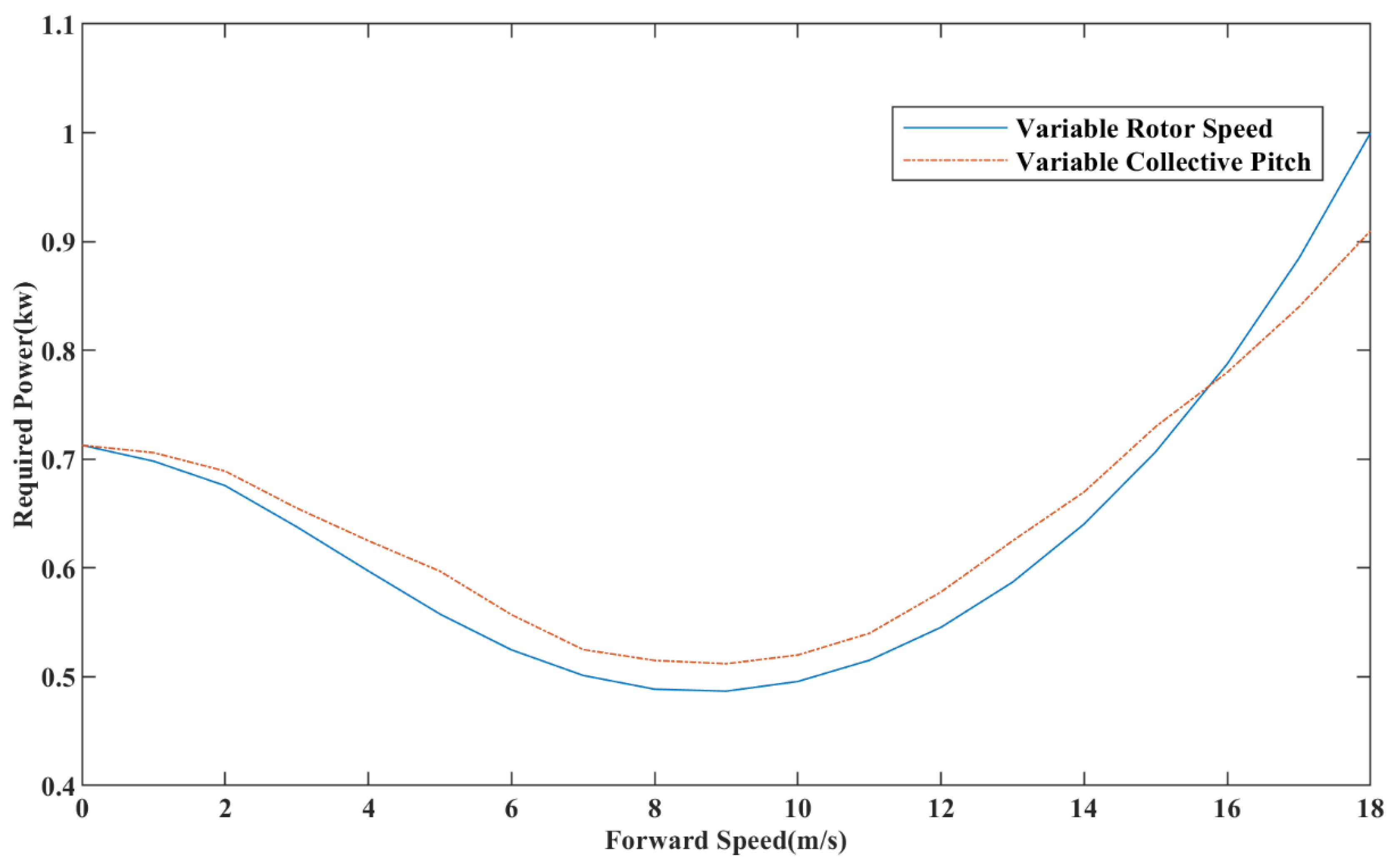
4. Comparison of Required Power of Variable Speed and Variable Total Distance

After proving the accuracy of the algorithm, this paper compares the required power of variable-speed coaxial helicopter and variable collective-pitch coaxial helicopter at different forward flight speeds, as shown in Figure 4. Among them, it is specified that the power of the variable-speed curve and variable total distance curve is the same in hovering. That is, the following are specified: the consistency of the rotor diameter, hovering rotor speed and hovering blade angle.

As is demonstrated in Figure 4, the two curves intersect when the forward flight speed is 15.4 m/s. Before the intersection point, the required power for the variable-speed coaxial helicopter is lower than that of the variable-pitch coaxial helicopter. When the power difference between the two is the largest, the required power of a variable-speed coaxial helicopter is 89% that of a variable total-pitch coaxial helicopter. After the intersection point, the required power of a variable-speed coaxial helicopter is higher than that of a variable-pitch coaxial helicopter, and the difference increases gradually.

It is worth noting that for the forward flight speed at the intersection of the two curves, the rotor speed with variable speed and variable total pitch corresponds to the hovering condition. It can be inferred that when the forward flight speed of the variable-speed coaxial helicopter increases, due to the characteristic that the rotor speed first decreases and then increases, the rotor type resistance first decreases and then increases, and the rotor efficiency first increases and then decreases, so that the variable-speed coaxial helicopter has a lower power demand near the cruise speed point than the variable-pitch coaxial helicopter, which improves the cruise flight time effectively, while the variable-pitch coaxial helicopter has lower required power at high speed.

Since this property is inherent in a helicopter, it can be considered that the above characteristics are available for variable-speed coaxial helicopters and variable collective-pitch coaxial helicopters with the same rotor diameter, hovering rotor speed and hovering blade angle.

5. Conclusions

In this paper, the model of a variable-speed coaxial helicopter is analyzed and deduced by the blade element method, a non-uniform inflow and empirical function method, and the equations containing 14 nonlinear equations are obtained. The equations are solved by Newton’s iterative method, and the parameter indexes after balancing are obtained. Through experimental verification, the deduced model is validated for its accuracy and robustness, and the correctness of the model has been testified. The maximum rotor speed error is less than 6%, and the maximum required power error is less than 5%. Finally, on the basis of the model, the required power curves of two coaxial helicopters are contrasted. When the rotor diameter, hovering total distance and hovering rotor speed is the same, the conclusions are as follows:

(1)

When the forward speed is less than the corresponding hovering rotor speed, the variable-speed coaxial helicopter has lower rotor power. This speed range applies to coaxial helicopters with strict flight time requirements, which have wide application.

(2)

When the forward speed is higher than the corresponding hovering rotor speed, the variable-pitch coaxial helicopter has lower rotor power. This speed range is applicable to coaxial helicopters that are required to perform high-speed flight missions.

In future, the research of the oscillation and flapping characteristics coupling problem, caused by the rotational speed in the yawing control of the variable-speed coaxial helicopter, will be considered thoroughly and in detail.

References

1. Xia, Q.; Xu, J. Load modelling and experimental verification of variable speed coaxial rotor. Exp. Mech. 2012, 27, 433–439. [Google Scholar]
2. Cheney, M.C.J. The ABC helicopter. J. Am. Helicopter Soc. 1969, 14, 10–19. [Google Scholar] [CrossRef]
3. Coleman, P. A Survey of Theoretical and Experimental Coaxial Rotor; NASA Technical Paper 3675; NASA: Washington, DC, USA, March 1997.
4. Leishman, J.G.; Ananthan, S. An optimum coaxial rotor system for axial flight. J. Am. Helicopter Soc. 2008, 53, 366–381. [Google Scholar] [CrossRef]
5. Leishman, J.G.; Bhagwat, M.J.; Bagai, A. Free-vortex filament methods for the analysis of helicopter rotor wake. J. Aircr. 2002, 39, 759–775. [Google Scholar] [CrossRef]
6. Griffiths, D.; Ananthan, S.; Leishman, J. Predictions of Rotor Performance in Ground Effect Using a Free-Vortex Wake Model. J. Am. Helicopter Soc. 2005, 50, 302–314. [Google Scholar] [CrossRef]
7. Nagashima, T.; Nakanishi, K. Optimum performance and wake geometry of the co-axial rotor in hover. In Proceedings of the 7th European Rotorcraft and Powered Life Forum, Garmisch-Partenkirchen, Germany, 8–11 September 1981. [Google Scholar]
8. Brown, R.E.; Kim, H.W. Coaxial Rotor Performance and Wake Dynamics in Steady and Manoeuvring Flight. In Proceedings of the American Helicopter Society 62nd Annual Forum, Phoenix, AZ, USA, 9–11 May 2006. [Google Scholar]
9. Qi, H.; Xu, G.; Lu, C.; Shi, Y. A study of coaxial rotor aerodynamic interaction mechanism in hover with the high-efficient trim model. Aerosp. Sci. Technol. 2019, 84, 1116–1130. [Google Scholar] [CrossRef]
10. Ramasamy, M. Measurements comparing hover performance of single, Coaxial, Tandem, and tilt-rotor configurations. Annu. Forum Proc.—AHS Int. 2013, 4, 2439–2461. [Google Scholar]
11. Passe, B.; Sridharan, A.; Baeder, J. Computational investigation of coaxial rotor interactional aerodynamics in steady forward flight. In Proceedings of the 33rd 33rd AIAA Applied Aerodynamics Conference, Dallas, TX, USA, 22–26 June 2015. [Google Scholar] [CrossRef]
12. Gessow, A. Effect of Rotor-Blade Twist and Plan-Form Taper on a Helicopter Hovering Performance; NASA: Washington, DC, USA, 1948.
13. Zhao, Q.; Liu, Y. Controllability Analysis of multi-rotor aircraft. J. Aeronaut. 2017, 38 (Suppl. S1), 163–170. [Google Scholar]
14. Song, Y.; Wang, H.; Lin, Z. Performance analysis and test of variable pitch and variable speed multi-axis rotor aircraft. J. Aeronaut. Dyn. 2018, 33, 1033–1040. [Google Scholar]
15. López-Martínez, M.; Ortega, M.G.; Vivas, C.; Rubio, F.R. Nonlinear L 2 control of a laboratory helicopter with variable speed rotors. Automatica 2007, 43, 655–661. [Google Scholar] [CrossRef]
16. Belmonte, L.M.; Morales, R.; Fernandez-Caballero, A.; Somolinos, J.A. A Tandem Active Disturbance Rejection Control for a Laboratory Helicopter with Variable-Speed Rotors. IEEE Trans. Ind. Electron. 2016, 63, 6395–6406. [Google Scholar] [CrossRef]
17. Zhou, G.; Hu, J.; Cao, Y.; Wang, J. Study on flight dynamics simulation mathematical model of coaxial helicopter. J. Aeronaut. 2003, 24, 293–295. [Google Scholar]
18. Zhou, G.; Hu, J.; Cao, Y.; Wang, J. Study on load calculation model of twin rotors of coaxial helicopter. J. Aeronaut. Dyn. 2003, 18, 343–347. [Google Scholar]
19. McAlister, K.W.; Tung, C. Experimental study of a hovering coaxial rotor with highly twisted blades. In Proceedings of the American Helicopter Society International Annual Forum, Montreal, QC, USA, 29 April–1 May 2008; Volume 3, pp. 1765–1781. [Google Scholar]
20. Chen, R. A survey of nonuniform inflow models for rotorcraft flight. Flight Dyn. Control Appl. 1990, 14, 147–184. [Google Scholar]
21. Johnson, W. Helicopter Theory; Dover Publications: New York, NY, USA, 1980; pp. 121–139. [Google Scholar]
Figure 1. (a) Experimental flight test. (b) Schematic of the configuration.
Applsci 12 09534 g001
Figure 2. Variation of rotor speed of trim with the increasing forward flight speed compared (calculated value) to the actual rotor speed of the verification aircraft (experimental value).
Applsci 12 09534 g002
Figure 3. Variation of the calculated required power of trim with the increasing forward flight speed (calculated value) compared to the actual required power of the verification aircraft (experimental value).
Applsci 12 09534 g003
Figure 4. The variation in required power to the forward speed between variable rotor speed coaxial helicopter and variable collective-pitch coaxial helicopter.
Applsci 12 09534 g004