1. Introduction
One of the main problems in the design of neural networks is the selection of the structural parameters of the network and their corresponding values before performing the training. In this work, the robust design artificial neural network (RDANN) methodology is used. The main focus of this methodology is based on reducing the number of experiments that can be carried out using the factorial fractional method, a statistical procedure based on the robust design philosophy proposed by Genichi Taguchi. This technique allows one to set the optimal settings on the control factors to make the process insensitive to noise factors [
1,
2].
Currently, the selection of the structural parameters in the design of artificial neural networks (ANNs) remains a complex task. The design of neural networks implies the optimal selection of a set of structural parameters in order to obtain greater convergence during the training process and high precision in the results. In [
1], the feasibility of this type of approach for the optimization of structural parameters in the design of a backpropagation artificial neural network (BPANN) for the determination of operational policies in a manufacturing system is demonstrated, where it is shown that the Taguchi method allows designers to improve the performance in the learning speed of the network and the precision in the obtained results.
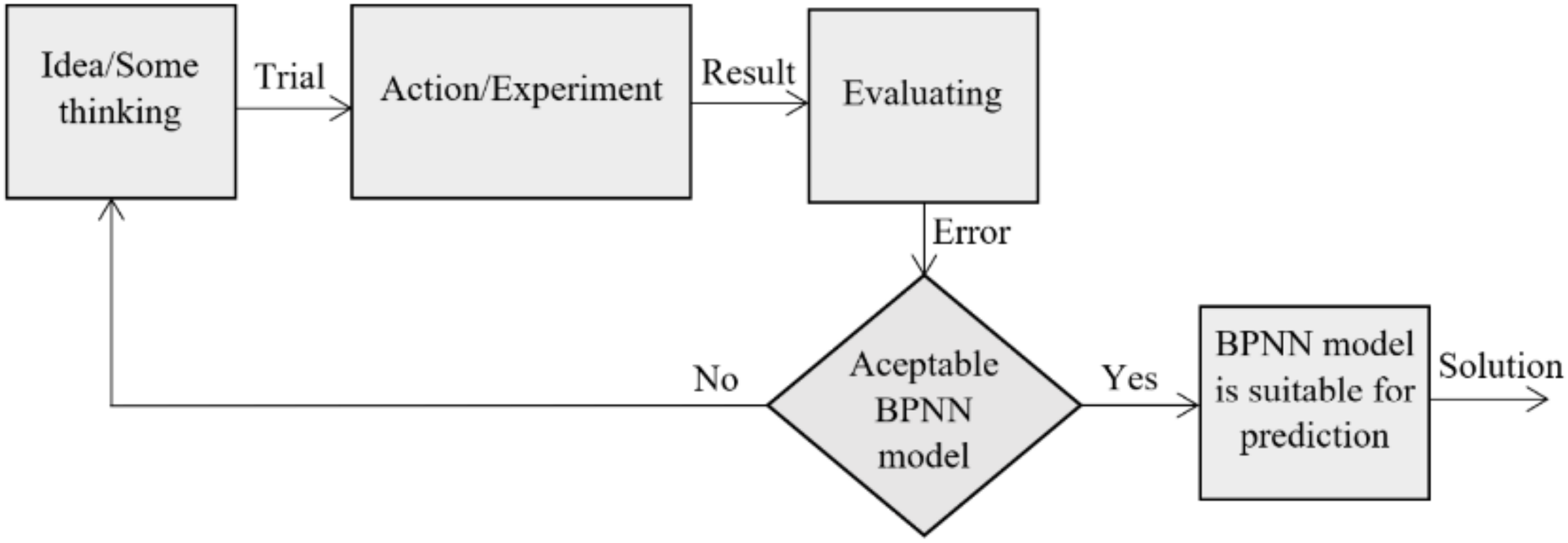
Most designers select an architecture type and determine the various structural parameters of the chosen network. However, there are no clear rules on how to choose those parameters in the selected network architecture, although these parameters determine the success of the network training. The selection of the structural parameters of the network is generally carried out through the implementation of conventional procedures based on trial and error, as shown in
Figure 1, where a significant number of ANN models are generally implemented in comparison with other unconventional procedures [
3,
4,
5,
6].
In this case, if a desired level of performance is not maintained, the levels in the previously established design parameters are changed until the desired performance is obtained. In each experiment, the responses are observed in order to determine the appropriate levels in the design of the structural parameters of the network [
7].
A drawback in the use of this type of procedure is that one parameter is evaluated, while the others are kept at a single level, so the level selected in a variable may not necessarily be the best at the end of the experiment, since it is very likely that most of the layout variables involved will change their value. A possible solution could be that all the possible combinations in the parameters are evaluated, that is, to carry out a complete factorial design. However, the number of combinations can be very large due to the number of levels and previously established design parameters, so this method could be computationally expensive and time-consuming.
Due to all these limitations, the scientific community has shown special interest in the implementation of new approaches and procedures applied to the optimization of structural parameters in the search to generate better performance in ANNs [
8,
9,
10,
11,
12,
13].
Currently, ANNs can be trained to solve problems that can be complex for a human or a conventional computer, since they allow obtaining results with a high degree of precision and a significant reduction in error in real-time applications. In recent decades, the use of ANNs has been successfully applied in different fields, including pattern recognition, classification, identification, voice, vision, control systems, and robotics, the latter of which has raised special interest among researchers in the field, particularly the solution of the inverse kinematics in manipulators with six or more degrees of freedom, due to the great flexibility of control that they present for the execution of very complex tasks [
14,
15,
16,
17].
In [
18], a BPNN algorithm is proposed, optimized by Fruit Fly Optimization Algorithm (FOA), to find the solution of the inverse kinematics in a four-DOF robot, obtaining an output error range −0.04686–0.1271 smaller than that obtained by a BPNN. In [
19], a BPNN algorithm, optimized by means of particle swarm optimization (PSO), is studied to solve the inverse kinematic problem in a six-DOF UR3 robot applied in puncture surgery, where convergence in the precision of the results, as well as the speed and generalization capacity of the proposed network, is improved. In [
20], a deep learning approach is proposed to solve the inverse kinematics in a seven-DOF manipulator. The approach used allows it to be fast, easy to implement, and more stable, allowing less sensitivity in hyperparameters. In [
21], a combination of swarm intelligence (SI) and the product of exponentials (PoEs) is used to solve the inverse kinematics in a seven-DOF manipulator, where they are compared with the conventional inverse kinematics and standard PSO algorithms. In [
22], the main approach is based on a redundant manipulator inverse kinematic problem that is formulated as a quadratic programming optimization problem solved by different types of recurrent neural networks. In [
23], an approach is proposed to address the complexity of solving the inverse kinematics in a seven-DOF serial manipulator through an algorithm based on the Artificial Bee Colony (ABC) optimization algorithm, where two control parameters are used in order to adjust the search to optimize the distribution of the sources. In [
24], an optimization approach is shown in the planning of the trajectories applied in a five-bar parallel robot for real-time control, minimizing the trajectory time and avoiding singularities in the parallel manipulator, achieving an error of less than 0.7° at the joints.
Factorial experimental design is a statistical technique used to identify and measure the effect that one variable has on another variable of interest. In 1920, R. A. Fisher studied multiple factors in the agricultural field to determine the effect of each factor on the response variable, as well as the effect of the interactions between factors on this variable. This method is known as the factorial design of experiments. Factors are variables that determine the functionality of a product or process and significantly influence system performance and can usually be controlled. To evaluate the impact of each variable, the factors must establish at least two levels; therefore, given
factors with
levels, a complete factorial design that includes all the possible combinations between these factors and levels will produce a total of
experimental runs. Obviously, as
or
increases, the number of experiments may become unfeasible to carry out, since a significant number of factors would imply a large number of experiments. For this reason, fractional factorial designs have been introduced, which require only a fraction of a run, unlike a complete factorial design, and which allow estimating a sufficient number of effects [
25,
26].
Genichi Taguchi is considered to be the author of robust parameter design through a procedure focused on reducing variation and/or sensitivity to noise in the design of products or processes, which is based on the concept of fractional factorial design. Through the implementation of orthogonal arrays (OA) and fractional factorial design, it is possible to analyze a wide range of parameters through a reduced number of experiments, ensuring a balanced comparison between the factors involved and the interaction with their different levels [
2,
27,
28].
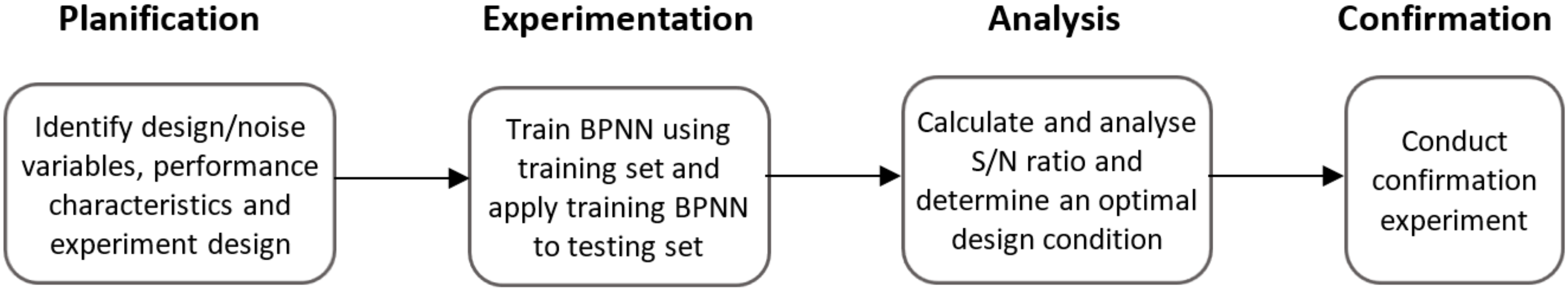
The Taguchi method is applied in four stages:
Selection of design and noise variables. In this stage, the most important parameters for the product/process are considered, taking into account the quality characteristics. Generally, there are variables that can be controlled by the user and others that cannot. These types of variables are known as design and noise factors, respectively, which have an important influence on the operation of the product/process. They can be determined mainly by answering the following questions: What is the optimal design condition? What factors contribute to the results and to what extent? What will be the expected result?
Design and experimentation. An OA is established, which contains the organization of the experiment taking into account the levels established for each of the factors in order to minimize the effects produced by noise factors. In other words, the adjustments made to the factors must be determined in such a way that there is the least variation in the response of the product/process, and the mean is established as close as possible to the desired objective. The OA allows the implementation of a balanced design in the weighting of the pre-established levels for each factor involved since it is possible to evaluate various factors with a minimum number of tests, obtaining a considerable amount of information through the application of few tests. The mean and variance of the response obtained in the OA configuration are combined into a single performance measure known as the signal-to-noise ratio (S/N).
Analysis of results. The S/N ratio is a quality indicator by which the effect produced on a particular parameter can be evaluated. The variation in the response obtained in dynamic characteristics, the S/N ratio, is shown below in the following equation:
where
is the square of the largest value of the signal, and
represents the root mean square deviation in the performance of the neural network, or in other words, the mean square of the distance between the measured response and the best fit line. A valid robustness measure is related to obtaining the highest values in the S/N ratio, because the configurations of control factors that minimize the effects on noise factors can be identified.
Execution and confirmation of tests in optimal conditions. In this stage, a confirmation experiment is carried out by performing training with optimal design conditions in order to calculate the performance robustness measure and verify if this value is close to the predicted value.
Inverse Kinematics with ANNs
During the last decade, robotics had an outstanding development in the industry, particularly in aerospace, military, and medical areas, among others, especially in manipulators with a large number of degrees of freedom (DOF), due to their high flexibility and control to perform complex tasks [
17,
29,
30].
Modern manipulators, usually kinematically redundant, allow complex tasks to be solved with high precision in the results. These types of manipulators have at least six DOF, allowing greater flexibility and mobility to perform complex tasks. The complexity in manipulator control design based on an inverse kinematic solution approach can be computationally complex, due to the nonlinear differential equation systems that are usually present. Traditional methods with geometric, iterative, and algebraic approaches have certain disadvantages and can often be generically inappropriate or computationally expensive [
16,
31].
The ANNs present major advantages related to nonlinearity, parallel distribution, high learning capacity, and great generalization capacity, and they can maintain a high calculation speed, thus fulfilling the real-time control requirements. Consequently, various approaches have been proposed by the scientific community in the use of intelligent algorithms applied to the control of robotic manipulators such as the use of ANNs [
19,
20,
32,
33], genetic algorithms [
31,
33,
34,
35,
36,
37,
38], recurrent neural networks (RNNs) [
37], [
38], optimization algorithms [
18,
23,
39,
40], and the use of neural networks and optimization methods for parallel robots [
24,
41].
The organization of this work is as follows: In
Section 2.1, the kinematic model of the Quetzal manipulator is established.
Section 2.2 describes the procedure for generating the training and testing dataset.
Section 2.3 describes the implementation of the RDANN methodology for the optimization of structural parameters in the BPNN. In
Section 3, the results obtained are subjected to a reliability test stage through the use of a cross-validation method to verify that the dataset is statistically consistent. The results of training in the optimized BPNN show a significant improvement in the accuracy of the results obtained compared with the use of conventional procedures based on trial-and-error tests.
2. Materials and Methods
In this paper, a robust design model is presented through a methodological and systematic approach based on the design philosophy proposed by Genichi Taguchi. The integration of optimization processes and ANN design are methodological tools that allow the performance and generalization capacity in ANN models to be improved. In this study, an RDANN methodology was used, which was initially proposed for the reconstruction of spectra in the field of neutron dosimetry by means of ANNs [
7].
The RDANN methodology was used to estimate the optimal structural parameters in a BPNN to calculate the inverse kinematics in a six-DOF robot, where the main objective was the development of accurate and robust ANN models. In other words, it was sought that the selection of the structural parameters of the proposed model allows us to obtain the best possible performance in the network.
2.1. Kinematic Analysis
The robot called Quetzal is based on an open source, 3D-printable, and low-cost manipulator [
42]. The modeling and representation were carried out using the Denavit–Hartemberg (D–H) parameters to obtain a kinematic model through four basic transformations that are determined based on the geometric characteristics of the Quetzal manipulator to be analyzed [
43]. The D–H parameters are shown in
Table 1.
The basic transformations represent a sequence of rotations and translations, where the reference system of element
is related to the system of element
. The transformation matrix is given by Equation (2).
Carrying out the multiplication of the four matrices, Equation (3) is obtained:
where
is the D–H transformation matrix from coordinate system
to
.
is the rotation matrix representing a rotation
around the
axis,
is the translation matrix representing a translation of
on the
axis,
is the translation matrix representing a translation of
on the
axis,
is the rotation matrix representing a rotation
around the
axis,
is shorthand for cos
,
is shorthand for
, etc. The transformation matrices of each of the joints are multiplied to obtain the initial position of the end effector in the base reference system, as shown in Equation (4).
Therefore, the equation of the forward kinematics of the Quetzal manipulator can be expressed as shown in Equation (5).
As shown in Equation (5), the position of the end effector of the manipulator can be obtained from the angular values of the six joints of the manipulator. However, in practice, it is necessary to obtain the angles at each of the joints through a given position, so it is necessary to calculate the inverse kinematics, which can be expressed as shown in Equation (6).
Solving (4) gives the orientation and position of the final effector in regard to the reference system, as shown in Equation (7), where the position vector
and the orientation vector
.
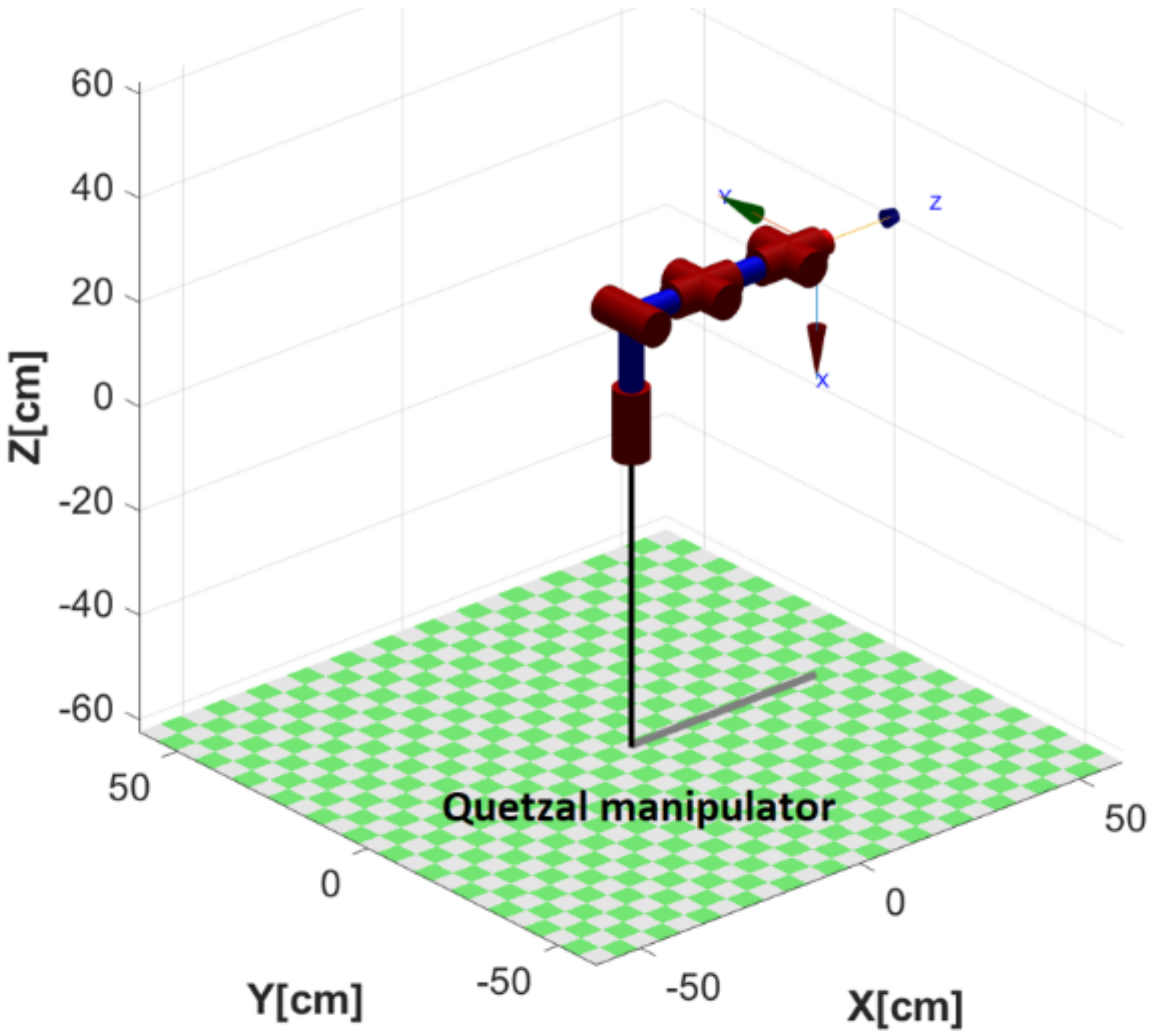
The graphic representation of the initial position of the Quetzal robotic manipulator is shown in
Figure 2 through a simulation carried out with the Robotics Toolbox for MATLAB software [
44].
2.2. Training and Testing Datasets
The dataset was generated from the equations obtained in the forward kinematics of the Quetzal manipulator. The variables involved in the proposed dataset were the orientation vector , the position vector , and the vector of joint angles , for a total of 18 variables.
Table 2 shows the ranges of movement established for each of the joints in the workspace of the manipulator. Dataset
was generated with a spatial resolution of
in a six-dimensional matrix with 18 variables involved. The total size of the dataset was 4,394,531,250 data, occupying an approximate physical memory space of 32.74 Gb due to the data class of type
used in the study, where the data are stored as 4-byte (32-bit) floating point values.
Figure 3 shows a graphical representation of the workspace using a 3D data scatter plot corresponding to the position vector
based only on the joints
and
, where it is possible to appreciate the workspace of the robotic manipulator without taking into account joint
. The illustrated workspace was generated from the forward kinematic equations as a function of the six joints.
In order to process the enormous volume of data in a conventional processor, a data reduction filter (DRF) based on linear systematic sampling (LSS) was applied to reduce the set to a size of 190.7 Kb in memory [
45]. The data were processed on an 8-core AMD Ryzen 7 5000 series processor with a base clock of 1.8 GHz, 16 GB of RAM, and integrated Radeon 16-thread graphics with a maximum clock of 4.3 GHz [
46]. The dataset and code are available in
Supplementary Materials.
Figure 4 shows the scatter matrices corresponding to the position dataset before and after applying the FRD filter, where a reduction of 99.99% of the data was obtained with a size of 24,410 data. In
Figure 4b, it is shown that the data maintain a constant and uniform distribution with respect to the dataset of
Figure 4a.
The data were normalized with a mean of zero in the range from −1 to 1 using Equation (8), where
is the data to normalize,
is the minimum value of the dataset,
is a value established by the difference between the maximum value and the minimum value of the dataset,
and
are the maximum and the minimum desired values for normalization.
2.3. Robust Design Methodology
Figure 5 shows the RDANN methodology based on the Taguchi philosophy that consists of four stages. The designer must know the problem and choose an appropriate network model, as well as the parameters involved in the design of the network for its optimization (planning stage). By implementing an OA and systematically training a small number of ANN models (experimentation stage), the response to be analyzed is determined using the S/N relationship of the Taguchi method (analysis stage). Finally, through a confirmation process, the best performance values of the model are obtained (confirmation stage).
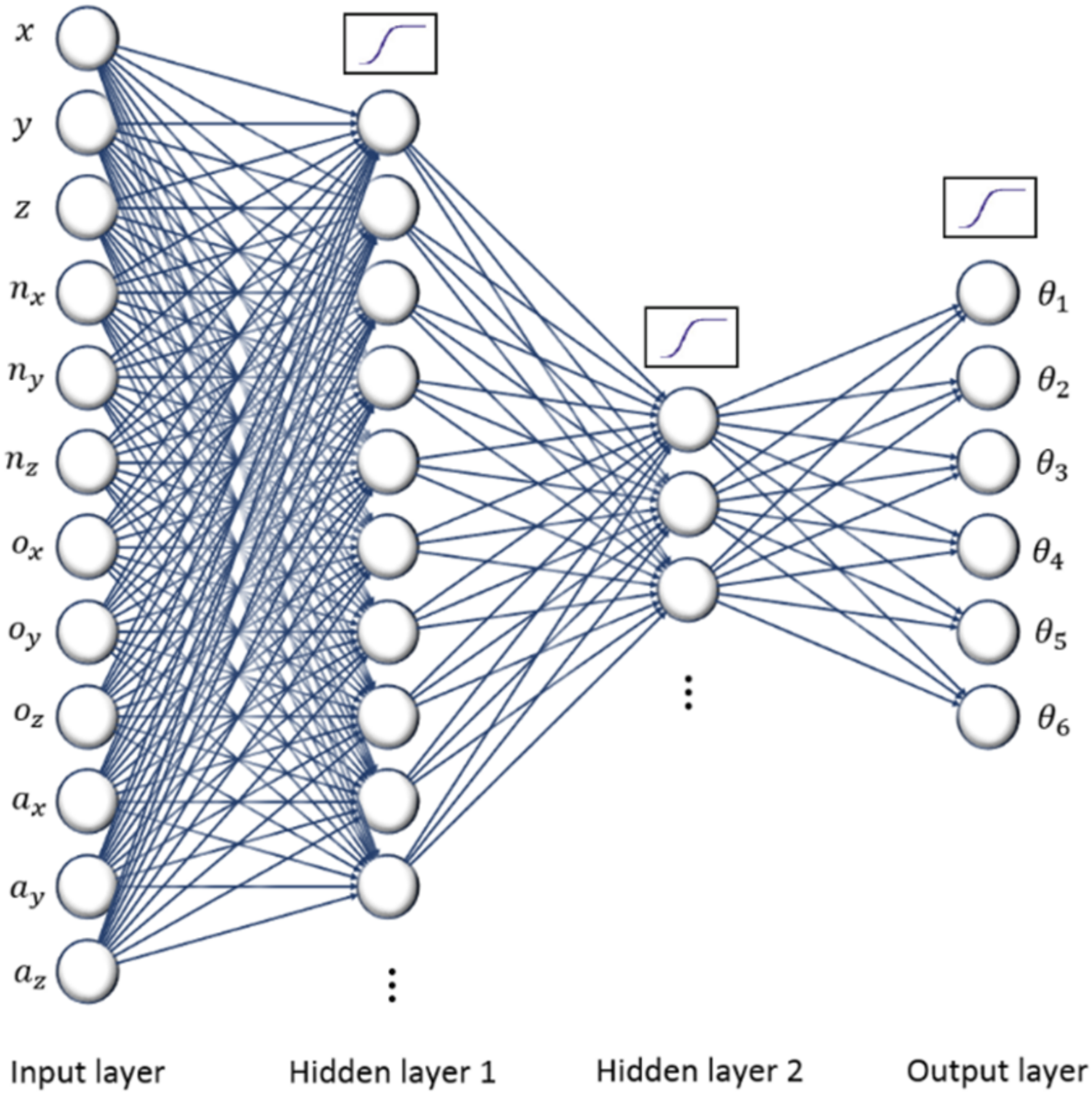
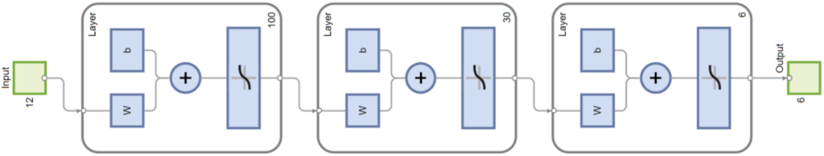
The graphic representation of the BPNN used in this work is shown in
Figure 6, with 12 input variables and 6 output variables that correspond to the position vector
and orientation vector
as input and the vector of joint angles
as output.
2.3.1. Planning Stage
In this stage, the design variables, noise, and the objective function are identified. The objective function is defined according to the purpose and requirements of the system. In this work, the objective function is related to the prediction or classification errors between the calculator data and the data predicted by the ANN model during the testing stage. The performance at the output of the ANN or the mean square error (MSE) is used as the objective function and is described in the following equation:
In this case, represents the number of attempts, represents the set of joint values that are predicted by the BPANN, and represents the set of joint values.
The design variables correspond to those that can be controlled by the user, such as the number of neurons in the first layer, the number of neurons in the second layer, the momentum constant, and the learning rate. By contrast, the noise variables are commonly not directly controlled by the user in most cases, such as the initialization of synaptic weights that are generally assigned randomly, the size of the training sets versus test sets, and the random selection of training and test sets. According to the requirements of the problem, the user can choose the factors related to variation in the system during the optimization process. Four design variables and three noise variables were selected because they were directly involved with the performance of the ANN, as described below in
Table 3 with their respective configuration levels.
In terms of variables,
is the number of neurons in the first hidden layer;
is the number of neurons in the second hidden layer;
is the momentum constant, which allows the stabilization of the updating of each of the synaptic weights taking into account the sign of the gradient;
is the learning rate, which allows us to define the cost that the gradient has in updating a weight because the increase or decrease in the synaptic weight is related to the magnitude of the proposed value, so it may or may not affect the convergence of the MSE, causing instability and divergence [
47].
is the initial set of weights,
is the size in proportions of the dataset, and
is the random selection from the training and testing set.
Once the variables and their respective levels were chosen, a suitable OA was chosen to carry out the training sessions. An OA is described as , where represents the number of rows, represents the number of columns, and represents the number of levels in each of the columns. In this experiment, the columns of the OA represent the parameters to be optimized, and the rows represent the tests carried out by combining the three proposed levels.
2.3.2. Experimentation Stage
The success in this stage depends on an adequate choice of the OA because, in this process, a series of calculations are carried out in order to evaluate the interaction and the effects produced between the variables involved through a reduced number of experiments. For the implementation of a robust design, Taguchi suggests the use of a configuration in two crossed OAs with
and
, as shown below in
Table 4.
2.3.3. Analysis Stage
Through the S/N ratio, a quantitative evaluation is carried out, where the mean and the variation in the responses measured by the ANN with different design parameters are considered. The unit of measure is the decibel, and the formula is described as follows:
In this case, is the root mean square deviation in the ANN performance. The best topology is considered when more signals and less noise are obtained; therefore, a high S/N ratio at this stage allows us to identify the best design values in the BPANN with the help of statistical analysis with the JMP software.
2.3.4. Confirmation Stage
In this stage, the value of the robustness measure is obtained based on the specifications and optimal conditions of the design. A confirmation experiment is carried out using the optimal design conditions that were previously chosen, in order to verify if the calculated value is close to the value predicted by the BPANN.
3. Results
In this work, the RDANN methodology was used for the optimal selection of the structural parameters in a feed-forward backpropagation network, known as BPNN, to find the solution to the inverse kinematics in a Quetzal robot. For the BPNN training, the “resilient backpropagation” training algorithm and were selected. In accordance with the RDANN methodology, an OA corresponding to the design and noise variables, respectively, was implemented in configurations and to determine the response to the tests during the 36 training sessions carried out.
The results obtained after applying the RDANN methodology are presented in the next sections.
3.1. Planning Stage
Table 5 shows the design and noise variables with their respective assigned values for the different levels proposed during the experiment.
The values for the three levels established in each of the tests regarding the number of neurons for the first hidden layer were , and ; for the number of neurons in the second hidden layer, they were , , and ; for the constant momentum, they were , , and ; and for the learning rate, they were , , and .
The values for the initial sets of weights were randomly determined at all three levels. The values set in the proportions of the dataset for level 1 were training and 30% testing; for level 2, they were 80% and 20%, and for level 3, they were 90% and 30%, respectively; finally, the random selection of the training and testing set for level 1 was ; for level 2, it was , and for level 3, it was .
3.2. Experimentation Stage
A total of 36 training sessions were carried out by implementing the OA in
and
configurations, where the network architectures were trained and tested, obtaining the results shown in
Table 6.
For the analysis of the S/N ratio, an analysis of variance (ANOVA) was performed using the statistical software program JMP. The S/N ratio and the mean value of the MSE are two of the specific criteria for determining the appropriate levels in the variables involved in network design, and their choice is determined through a series of validation procedures carried out in the next stage, as described below.
3.3. Analysis Stage
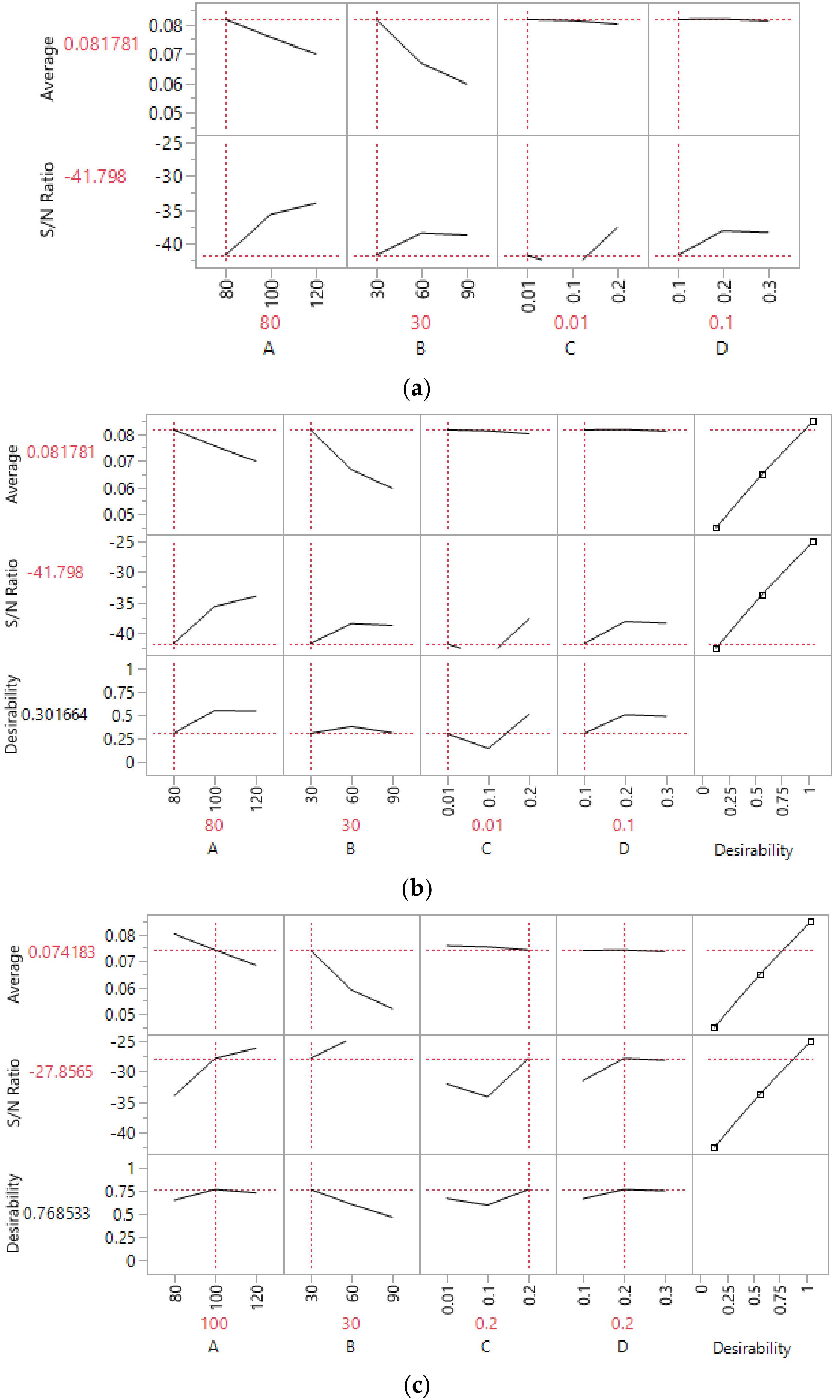
Figure 7a shows the best network topology obtained through the normal profile;
Figure 7b describes the best topology through the desirable profile, and
Figure 7c describes the best network topology using the maximized desirable profile. The three network profiles were obtained through statistical analysis in the JMP software to identify the optimal values in each of the proposed profiles. After performing the analysis of the S/N ratio, the values in which the levels for each of the variables involved were nearest to the average and S/N ratio red lines on the X axis were chosen, which are described in
Table 7.
For the choice of the best network profile obtained, three training sessions were carried out for each of the three profiles in order to contrast them based on the size of the training and test data and their generalization capacity, estimating the percentage of correct answers in the prediction of the data, obtaining the results shown in
Table 8.
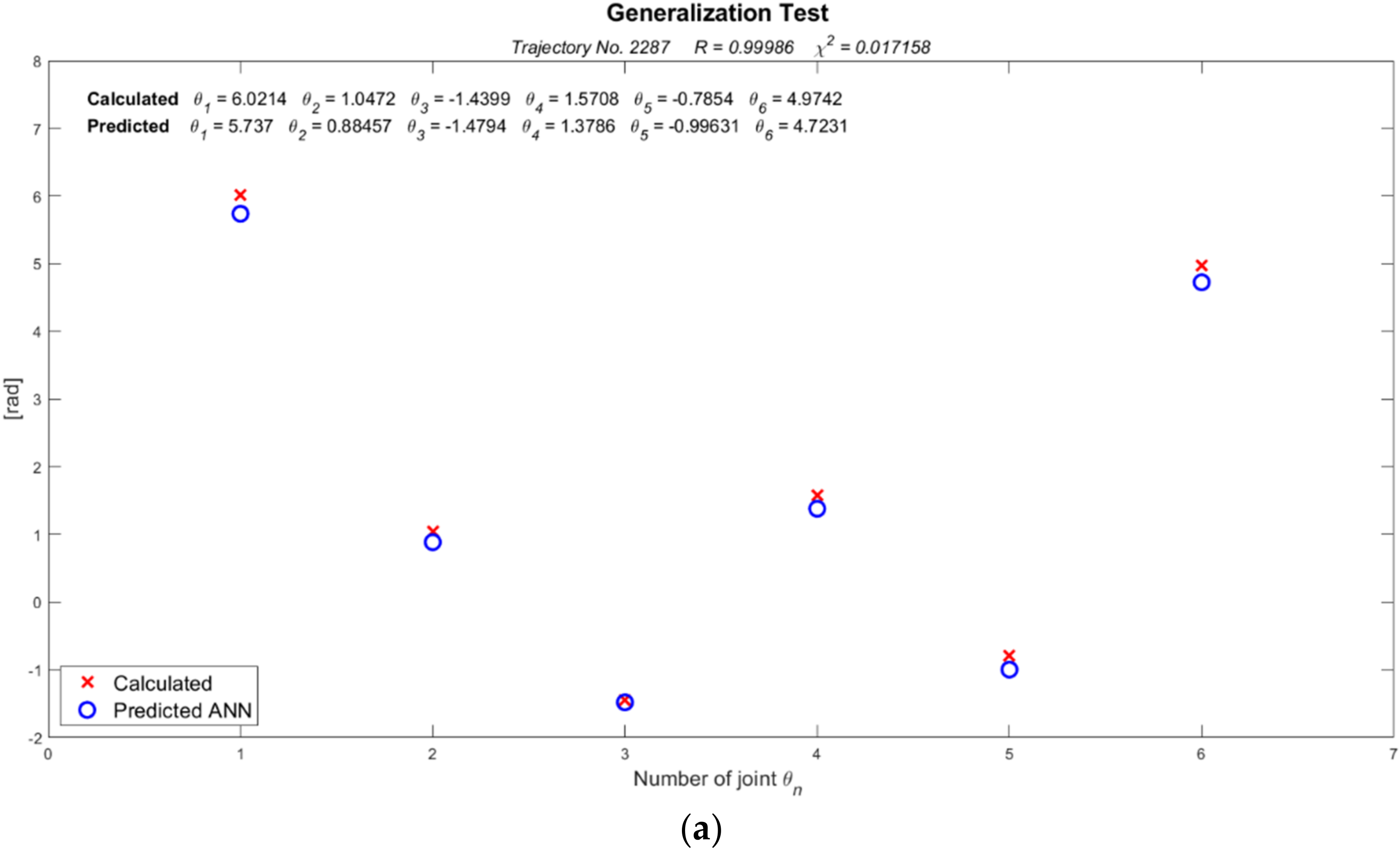
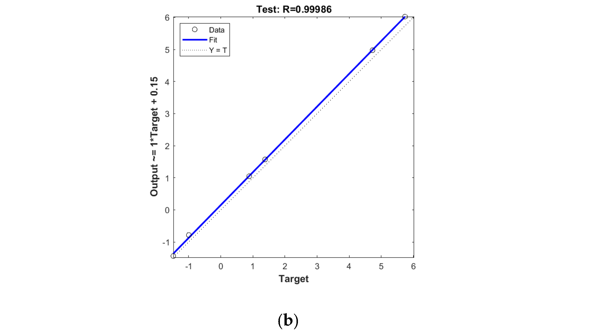
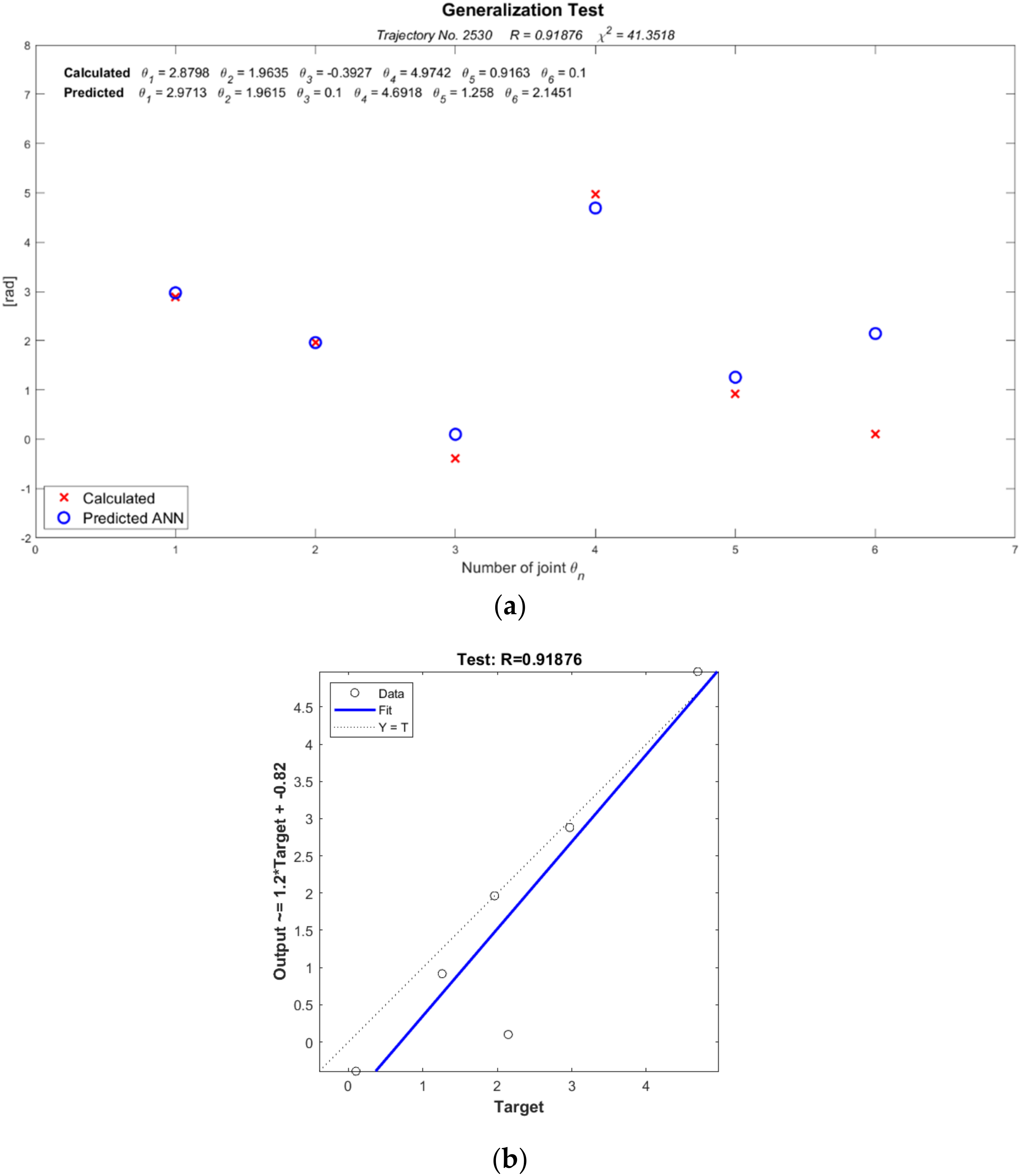
The best topology corresponds to the maximized desirable profile, with the percentage of obtained hits being 87.71% with a margin of error of less than 5% in the tests. Once the best topology was chosen, the statistical tests of correlation and chi-square were performed, showing the best and worst prediction of the network, as shown in
Figure 8 and
Figure 9, respectively.
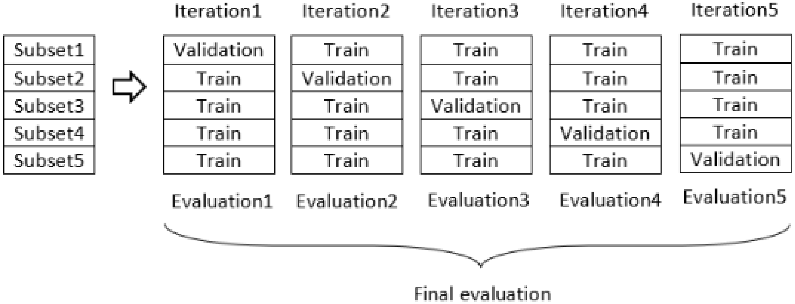
To determine if the predicted data are statistically reliable, the cross-validation method was used by splitting the training and testing datasets. The set was split into five subsets of the same size, as shown in
Figure 10. The validation subset in each training session was used to measure the generalization error, in other words, the misclassification rate of the model with data dissimilar from those previously applied during the training procedure. The cross-validation procedure was implemented on the training and testing datasets, and the average value of MSE and the standard deviation obtained were very close to those obtained in the confirmation stage [
48].
Table 9 shows the results obtained in the cross-validation process, where it is observed that the average training value was equal to 17.5099, the average percentage of hits considering an error of less than 5% was equal to 87.86%, and the average value of MSE was equal to 17.5099, with standard deviations of 1.5848, 1.8974, and 0.0059, respectively.
In relation to the three profiles analyzed, the choice of the appropriate levels for the structural parameters of the best network topology were those corresponding to the maximized desirable profile with 100 and 30 neurons, respectively, a momentum of 0.2, and a learning rate of 0.2.
Figure 11 shows the layered surface diagram of the neural network used in this work. The training was performed using MATLAB software. The ANN was composed of an input layer with 100 neurons, a hidden layer with 30 neurons, and an output layer with 6 neurons. All three layers used the activation function. The training algorithm used to adjust the weighting of the synaptic weights was
.
3.4. Implementation Results Compared with Simulation Results
Table 10 shows the measurement of the 10 trajectories predicted by the Quetzal manipulator and the error generated in comparison with the calculated trajectory. To analyze the data, 10 trajectories were chosen from the training dataset, and the simulation of each of them was carried out in order to obtain the distance traveled from the initial position to the final point.
The greatest error observed was in trajectory number 236, with a value of 7.7% compared with the calculated one, while for trajectory number 6, the error was 1.1% compared with the calculated one. A mean error of 3.5% was obtained for the implementation of the 10 physically realized trajectories using the low-cost (approximately USD 1500) 3D-printed Quetzal manipulator.
3.5. Comparative Analysis
Table 11 shows the values obtained in the design of the optimized BPNN in comparison with the BPNN based on trial and error and other methods used in the optimization of the structural parameters in ANN. As can be seen, the conventional BPNN method based on trial and error shows a greater difficulty in determining the optimal parameters, whereas the optimized BPNN results in a shorter time in the training process than the other methods; in addition, it involves noise parameters that are necessary to generate greater robustness in the network design.
4. Conclusions and Discussion
Various approaches and powerful learning algorithms of great value have been introduced in recent decades; however, the integration of the various approaches in ANN optimization has allowed researchers to improve performance and generalizability in ANNs. The results of this work revealed that the proposed systematic and experimental approach is a useful alternative for the robust design of ANNs since it allows simultaneously considering the design and the noise variables, incorporating the concept of robustness in the design of ANNs. The RDANN methodology used in this work was initially proposed in the field of neutron dosimetry, so it was adapted for implementation in the field of robotics, allowing us to improve the performance and generalization capacity in an ANN to find the solution to the inverse kinematics in the Quetzal manipulator.
The time spent during the network design process was significantly reduced compared with the conventional methods based on trial and error. In the methods that are generally proposed by the previous experience of the researcher, the design and modeling of the network can take from several days to a few weeks or even months to test the different ANN architectures, which can lead to a relatively poor design. The use of the RDANN methodology in this study allowed the network design to be carried out in less time, with approximately 13 h of training, due to the orthogonal arrangement corresponding to the 36 training sessions performed using a conventional AMD Ryzen 7 5700 series processor with an integrated graphics card.
Depending on the complexity of the problem, the use of this methodology allows handling times ranging from minutes to hours to determine the best robustness parameters in the network architecture. Therefore, it is possible to streamline the process and reduce efforts, with a high degree of precision in network performance. The use of the RDANN methodology allowed the analysis of the interaction between the values in the design variables that were involved, in order to consider their effects on network performance, thus allowing a reduction in the time and effort spent in the modeling stage and speeding up the selection and interpretation of the optimal values in the structural parameters of the network. The quality of the data in the training sets, without a doubt, can significantly help to increase the performance, generalization capacity, and precision of the results obtained. Although the proposed method was implemented and tested in a low-cost manipulator in this study, in future work, we plan to implement it in an industrial-type robot controller. The implementation of the proposed method in parallel robotic manipulators, where the solution of the kinematics is more complex, is also considered.


 ,
, 


