1. Introduction
Energy is one of the most important aspects in the development of our society. Easy and cheap access to energy has always been a challenge, and nowadays there is the added factor of environmental pollution that can be caused by the type of energy source that is used. Carbon and gas-based energy is increasingly being curtailed in favour of green energy, such as that derived from the sun, tides, or wind. These renewable energy sources are an excellent choice because they are clean and can occur in various forms over a large geographic area. This is another important point for democratising access to energy, as many countries do not have access to carbon-based energy.
One of the biggest financial impacts on the cost of electricity (LCOE) of wind turbines (WT) is associated with operation and maintenance tasks. Several schemes have been proposed to reduce O&M costs. An overview of the different strategies can be found in [
1,
2,
3]. One of the options is to detect abnormal behaviour in WTs as early as possible, before failures occur. Since the malfunction can then be corrected more quickly and without major damage to the subsystems of WT, the electricity production costs decrease. There are several ways to deal with this, and in this paper a data-driven normal behaviour model (NBM) based on our previous work [
4] is used to investigate how time scale affects the results of the prediction system.
Typically, turbines have a Supervisory Control and Data Acquisition (SCADA) system that provides a range of data to monitor the status of subsystems. More specifically, a SCADA system gathers data from the wind turbines’ systems and subsystems, and analyses and visualises data. Operators can view important measurements such as temperature, rotation speed, power consumption, etc., without having to visit each wind turbine on site. A typical SCADA architecture has the following five main elements: (i) Human Machine Interface (HMI) software for visualisation, which is a dashboard through which operators can interact with a WT, system, or device, and track real-time. These user interfaces allow full remote control of the equipment. (ii) Historian software, which are responsible for logging and storing asset data allowing operators to reference historical trends for analysis and reporting by providing a complete picture of their operations. (iii) Supervisory system, the core of SCADA systems, are servers and software that gather sensor data and send control commands to connected field devices. The supervisory computer also communicates with the human-machine interfaces to visualize real-time data for users. (iv) Communication infrastructure, which enables data transmission between the programmable logic controllers (PLC), remote terminal units (RTU), and the master SCADA system. (v) Finally, the remote terminal units and programmable logic controllers, which are the physical devices that both gather telemetry data from the wind turbines and execute control programs. Sensors placed in different parts of the WT are responsible for collecting this data, which is obtained through statistics such as minimum value, maximum value, average value, and standard deviation of various physical measurements, such as temperature, pressure, voltage, current, etc., in different parts of the subsystems. Over the past decade, the importance of SCADA data for predictive maintenance and monitoring has increased significantly. In [
5,
6,
7,
8] some of the first attempts to use SCADA data for turbine condition monitoring can be seen. The way to analyse and extract information has improved significantly since the early days. Several algorithms are available in the literature to assess the states of all principal components using different approaches based on statistical analysis, machine learning, and deep learning [
9,
10,
11]. SCADA benefits from the highly desirable characteristics of wide availability, highly standardized formats, and low cost.
Supervised learning and classification problems require complex pre-processing pipelines for data preparation. First, reliable data labels must be assigned. Next, the data must be accurately filtered and often enhanced by generating additional features that can highlight interesting features in the data. Finally, a classification model can be trained and used for prediction. All these steps are time-consuming. Label assignment is most likely the most important and the most time-consuming step. Work orders and alarm logs can be used to assign labels, but the lack of a standard format, the free-text nature of the data, and common discrepancies in the information make it difficult to automate processes and ensure that labels are reliable. Regression requires a less complex pipeline, filtering data through labels rather than defining groups. A common challenge in regression tasks is to choose a distance metric to use to quantify the quality of predictions and to assess the difference between predicted and observed values when analysing new data. Analysing the results, choosing the number of clusters, and interpreting them is important and non-trivial, but clustering and anomaly detection are much easier to train and easier to pre-process the pipeline. In general, the methods for condition monitoring with SCADA data use several strategies such as signal trending, modelling with neural networks, or some physical models. To conduct some form of exploration or analysis of the data, machine learning-based algorithms are commonly used. For example, in [
12] the authors use machine learning on SCADA data to predict WT failures. However, because the scenario is very unbalanced, with most of the samples coming from one class, such classifiers tend to perform poorly [
13]. For this reason, the authors in [
4] propose to use normality models to predict a (real) variable from a subsystem based on the rest of the variables and comparing them with the actual variable to determine if the predicted variable was consistent with the real one. If the predicted diverged from the real one, this divergence indicated a deterioration of the sub-system. In this initial work, Extreme Learning Machines (ELM) were used for implementation, while the results were compared with other widely used methods, such as Partial Least Squares (PLS), Support Vector Machines (SVM) or Deep Artificial Neural Networks (DANN). ELMs were selected because they can be trained very easily and fast, which is a very interesting feature. If the system has a fast training stage, the parameters can be adjusted very rapidly so that the models can be adjusted and fine-tuned in a very short time. Interested readers can find more details in [
4].
The SCADA system usually collects data at 10-min intervals. However, other intervals are also possible, such as 5 min. Recently, some work has investigated the effect of sampling frequency when collecting data in SCADA systems. For example, in [
14] a wind turbine performance monitoring technique based on high-frequency SCADA data is presented. The sampling frequency is 4 s and it is shown that its use is beneficial for performance monitoring, because the use of 5-min data tends to smooth this variation and does not provide the degree of detail provided by high-frequency data. Fischer and Coronado’s suggestions in [
15] also highlight that 5-min data is not appropriate as a standardised solution. Nevertheless, it is a valuable and relevant tool for the development of condition monitoring systems (CMS). High frequency data appears to be a good option for CMS development and to bring more information for wind farm management, as pointed out in [
16].
In any case, ANNs of different types have shown their usefulness in the construction of these regression models. The idea behind it is simple. Periods of good operation of the machines to be modelled are determined and a model is built that predicts one or more outputs (targets) from other input variables. The most direct way is to build a regression system that predicts the targets. Once the model is trained, it is kept running in the test part. The error between estimation and measurement gives an idea of how well the system is working. A small error, of the order of the error made in the training phase of the system, means that the system is working correctly. However, when systems deteriorate, measurements and calculations begin to diverge. Then, the error starts to grow and this increase provides an early signal of a possible failure.
An increasingly popular and effective methodology for assessing the condition of turbine components are so-called normality models. They attempt to capture the relationship between a set of input variables and one or more target signals, which should be able to determine the condition of the analysed component. An important step in normality models is the filtering of the data to determine a subset of records that can be labelled as normal data. Event and alarm records are often used for this task. Next, a set of inputs and a target variable can be chosen, and an algorithm is fitted to the data. The goal is to infer the model that describes the normal operating conditions of the monitored component, and then use it to track deviations between the expected and observed behaviour of the tracked variable. This approach is quite common in the wide world of predictive maintenance, not only in wind turbine monitoring. One of the first, and most likely the most influential, application of normality models to wind turbine monitoring is presented in [
5]. Neural networks are a popular choice due to their ability to model complex relationships in data; some examples are provided in [
17,
18,
19]. Other authors have compared the performance of neural networks with standard machine learning algorithms, and regression models [
9,
20] or alternative neural networks such as Extreme Learning Machines [
4]. Normality models allow capturing the complex relationships that can exist between turbine operating parameters such as temperatures, pressures, etc., and external factors such as wind speed and ambient temperature. Improved modelling capability comes at the cost of reduced interpretability compared to signal trending methods. The tuning of the models, the definition of the best hyperparameters, and the architecture are not trivial and require knowledge of data modelling and machine/deep learning. Normality models in wind turbines work best when they model individual turbines [
4,
21]. When a generic model is built for all the turbines in the wind farm, despite being of the same type and manufacturer, they always perform worse. The performance of the turbines depends very strongly on their location, when compared between wind farms, and significantly within the wind farm itself. In addition, when building models using SCADA data, some precautions must be taken. The main one is to train the normality model with correct data; that is, making sure that the turbine works properly in different operating regimes and preferably in all seasons of the year, being sure that no malfunctioning sections of the machine are introduced as they would bias and perturb the model. SCADA data is cheap to obtain and practically available on all farms, but has low latency (5–10 min), so it is appropriate to focus on slow time-varying targets. SCADA data are also characterised by outliers and missing data. The number of variables that the SCADA system captures is extremely high.
In this paper, a way to determine the good performance of wind turbines is explored, by comparing the variables of nearby machines of the same wind-farm and at the same time instant, since it has been observed that, despite slight differences, the climatic conditions (wind, temperature, humidity, etc.) are very similar as they are geographically very close. When plotting them synchronised, the patterns are reproduced, as explained in
Section 3.4. From here, a reference signal is calculated and used to compare the rest of the signals, extracting the signal difference between this reference signal and the (real) signals of each turbine. From experiments, it has been observed that the signal difference is stable over a range of values when the turbine is working properly, but, when it grows and remains stable over time, it is indicative of a malfunctioning system.
To our knowledge, no work has examined the impact of estimating the values of turbine variables using information from neighbouring turbines geographically close to the one under analysis. The interest of this strategy is primarily to simplify the models and create a baseline to be able to detect deviations from it that indicate a malfunction of a turbine. This work investigates this strategy in detail and demonstrates experimentally that it provides simple but very useful information for monitoring wind turbine farms.
The malfunction of a particular system or subsystem in a wind turbine is extremely rare, so very few cases are available. Another problem in this field is the inconsistency of labelling. Ultimately, the use of a normality model together with a regression technique instead of classification-based models seems to be a good strategy. The critical point is to train a normality model using data records belonging to different operating regimes, when the turbines are operating correctly. If accurate models are to be developed, it is necessary to have large data records to correctly represent the different conditions that may occur, for example in changing wind or weather conditions.
The article is organised as follows. In
Section 2, how the signals of the different turbines show very clear time-varying patterns is illustrated from examples with real data. This observation is evident from a temporally limited fragment of signals from the generator system. Such observations motivate the study. Taking advantage of the representation, problems associated with SCADA data processing such as the presence of outliers or missing data, are presented and analysed. In
Section 3, Materials and Methods, the database used in this work, the data synchronisation method, the method used to filter outliers, and the way the reference signal is generated, are presented.
Section 4 is devoted to the results of analysing each turbine with the proposed method. Finally, the article ends with a brief discussion in
Section 5 and with the conclusions in
Section 6.
A list of acronyms used in this work is included before the References to facilitate the reading of the manuscript.
2. Preliminary Observations
When observing and comparing the evolution over time of the same variable for all wind turbines operating correctly in a wind farm, a clear pattern of change can be noticed. This result is expected as the turbines are identical and are so close geographically that the operating conditions are very similar between them. Furthermore, the SCADA data are averages of the variables over 5 min (in our data), so that the higher frequency variations are lost in this operation.
Thus, although this pattern of joint variation appears in all the variables, it becomes highly evident when the represented magnitude is of slow variation, as in the case of temperature or pressure measurements.
To illustrate the coupling of the signals through a representation, the evolution of the same variables in perfect time alignment is depicted to see the near-ideal synchronisation when the WTs are working correctly, but are decoupled otherwise. This observation is fundamental to develop a method based on neighbour observations.
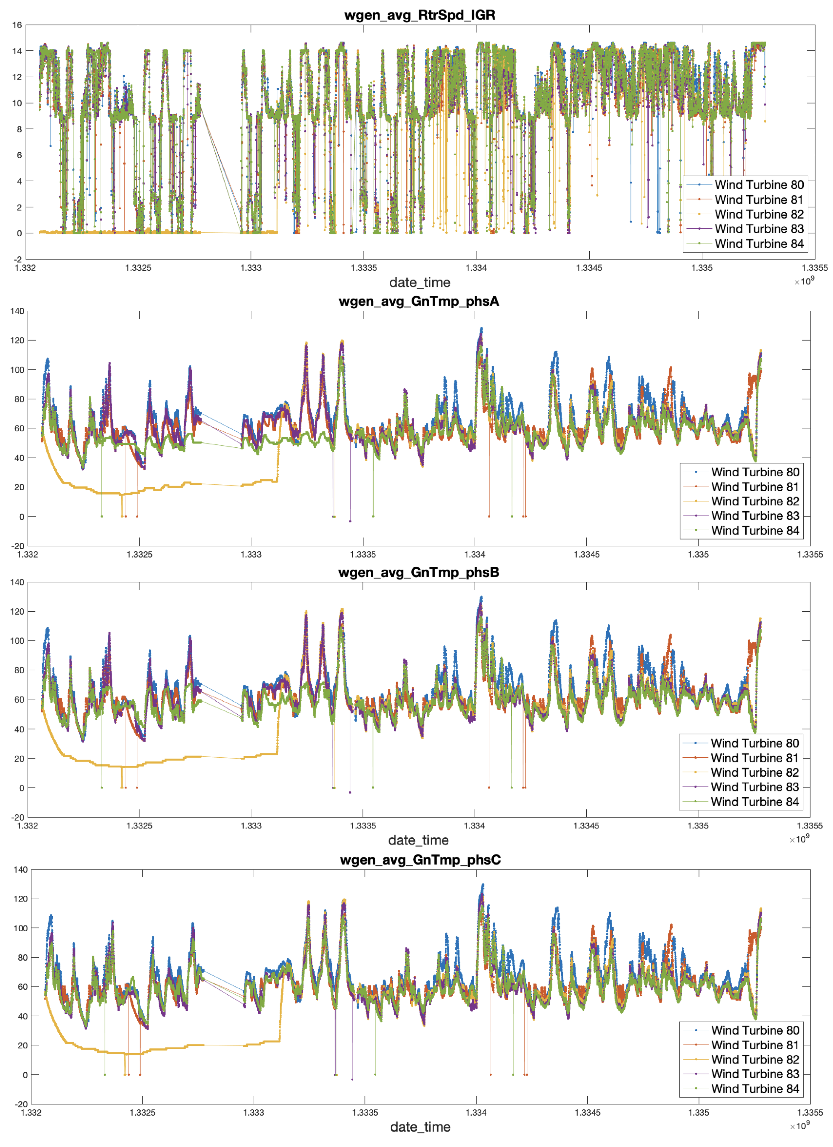
Figure 1 shows, for the same time interval, four magnitudes of the generator system of all the turbines of the park. The first signal corresponds to an angular velocity:
wgen_avg_RtrSpd_IGR and the lasts three signals correspond to the temperatures:
wgen_avg_GnTmp_phsA,
wgen_avg_GnTmp_phsB,
wgen_avg_GnTmp_phsC. In fact, these are the first four variables that appear in the database. See
Section 3 for an explanation of the names of the variables.
The upper graph in
Figure 1 shows the rotor speed
wgen_avg_RtrSpd_IGR of all superimposed wind turbines in perfect time alignment, following a switching pattern due to the presence of wind that causes the wind turbine to produce power or to be stopped. It is interesting to note that, while the magnitudes of the well-functioning machines fluctuate similarly, the WT82 (in yellow) is decoupled from the general operation for a time interval. That is, during a time interval the values of the WT82’s signal
wgen_avg_RtrSpd_IGR take values close to zero, indicating that the turbine shaft does not rotate (it is stopped), when the rest of the turbines maintain a pattern of activity. From now on, this signal will be used to determine the status of the WTs. The next three signals in
Figure 1 are the temperatures, which are closely coupled to each other in such a way that it takes careful observation to see that they are different. Thus, it can be observed that the temperature of turbine WT82 drops to room temperature levels during the interval where the rotor speed of WT82 (the signal
wgen_avg_RtrSpd_IGR in the upper plot, also in yellow) becomes zero, indicating that the turbine, despite the wind blowing, has been stopped, possibly due to a fault.
This observation illustrates that when the WTs work correctly, the magnitudes collected by the SCADA evolve synchronously between them, but when this is not the case, this synchrony is disrupted, and the signal wgen_avg_RtrSpd_IGR is useful to determine the WT state.
Figure 1 also points out two typical problems that appear in the SCADA databases. The first one is the presence of outliers and the second one is the lack of data in certain periods due to the failure of the SCADA system.
In
Figure 1, especially in the three temperature plots, the outliers are easily identifiable due to the physical impossibility of such a large variation. In this case it seems that the data has been poorly transmitted since each WT that presents an error—an outlier—is simultaneously shown in all the signals. Note that the outlier is represented by a certain colour (which also identifies each turbine). When the fault affects a magnitude of the turbine but not the rest of magnitudes, the fault can be attributed to a sensor fault. In
Figure 1, a general failure of the SCADA system can also be noticed, because there is a time interval in which no data is recorded, affecting all the magnitudes of all the turbines.
3. Materials and Methods
In the following sections, the experimental database is described. Because not all the sensors have all the data times, a temporal alignment method is also presented. Then, an outlier removing block is described and after that, the reference signal for all the WTs can be calculated, from which the deviation of each individual turbine will be extracted. This residue will be used to identify possible failures in the turbines. Finally, the Gearbox subsystem is analysed using the above-mentioned procedure.
3.1. Experimental SCADA Data
A comprehensive three-year SCADA database of five wind turbines of 2.5 MW Fuhrlaender, model FL2500, is presented. This turbine model consist of 10 different systems: grid, transmission, generator, converter, nacelle, hydraulic system, rotor, meteorological, turbine, and tower. The turbine signals are also organised into 10 groups, according to the system they belong to.
The data in this database were generated by the wind turbine SCADA and collected via an open communication platform (OPC) according to IEC 61400-25 format, which is the standard protocol used for communication between wind turbines and SCADA systems. Events and statistical indicators are recorded every five minutes. The values reported for each sensor are: Minimum, Maximum, Mean, and Standard Deviation. The database contains 312 analogue variables from 78 different sensors. The variables are stored with a name symbolising the (sub)system and the type of variable, separated by an underscore; the first term is the main physical system, e.g., generator = wgen, gearbox = wtrm, nacelle = wnac, etc. The second term is the type of variable of the 5-min interval, e.g., min = minimum, avg = average, etc. The third and fourth terms are the final name of the variable. Each of the events is labelled with a number. If the WT operates normally, the label is ‘0’. If there is a warning, the turbine is not stopped and the label is ‘1’. Finally, an alarm is indicated using ‘2’ as label, and in that case the WT is stopped. Alarms occur very sporadically in WT, as the turbine operates correctly most of the time. Therefore, it is common practice to combine warnings and alarms into a single class because a warning can precede a future alarm if the WT is not properly inspected. This reduces the problem to a two-class scenario. The aim is to identify in advance when a wind turbine starts operating with potential problems that could lead to a warning or alarm condition. In the experiments, only some of the system-related variables of the analysed subsystem are used. The database was provided by Smartive (
http://smartive.eu) (accessed on 20 April 2022) and has been used in other publications [
4,
21,
22,
23,
24].
All the data from the SCADA system is in a MySQL database, and the MATLAB Database Toolbox was used to download data from it (see
Table 1 for the exact dates of the data acquisition). So, all the processing has been done under a MATLAB 2021b environment running on a 2.4 GHz Intel Core i9 of 8 cores with 64 GB 2667 MHz DDR4 in macOS Monterrey.
In this contribution, signals from two different turbine systems, generation and transmission, are used. To show in context where each of the signals used belong and why they were chosen, two tables (
Table 2 and
Table 3) are organised.
First, to show the synchronous variation of the signals in
Section 2 and to introduce the method, (outliers filtering, pattern generation, etc.) in
Section 3.1,
Section 3.2,
Section 3.3 and
Section 3.4, four signals from the generator system are used (see
Table 2). This is a selection of three slowly varying temperature signals and one more quickly varying angular velocity signal that are used to determine the status of the WT.
Second, two signals from the gearbox subsystem are used.
The gearbox is a subsystem within the transmission system. Since a fault in the gearbox is expensive and difficult to repair, it is one of the subsystems that requires the most monitoring. Therefore, in this work, the gearbox subsystem is the one chosen to be monitored.
The presented method does not need a large number of signals to work properly. For this reason, the gearbox will be monitored from
Section 3.5 onward only with a temperature signal and a pressure signal with the additional support of the
(used to verify the status of the WT).
The temperatures are measured at different points of the gearbox chain and therefore different possibilities are available. In fact, having the complete analysis of all the signals of a subsystem is not difficult. Doing so can be used to try to isolate the fault within the subsystem or simply to reinforce the results. However, for the sake of clarity, an analysis with few signals is performed.
In
Table 3 the list of the temperature and pressure measurements collected in the transmission system is presented, using the name of the signals according to the note in which they appear in the database. The first 13 variables measure temperature in Celsius, and the last three correspond to pressure measurements. The variables used in the analysis are highlighted in bold.
3.2. Temporal Alignment of the Signals of the Ensemble of WTs
When extracting the signals from each of the turbines, it is observed that the number of samples differs slightly, so that if, for example, looking at the 10,000th sample of the same signal from each turbine, their data-times do not match. The first step of our method is therefore to temporarily align the signals of all turbines The turbine with the highest number of records is WT81 with 215,613 and the one with the lowest number of records is WT84 with 210,689. Therefore, the records whose data-time were not available for all turbines were removed. After completing the alignment process, 201,444 samples on all the turbines were available. This means that 0.0657% of samples from WT1 and 0.0439% from WT4 were removed. This is three orders of magnitude lower than the volume of data lost due to the general failure of the SCADA system.
3.3. Filtering of Outliers
Another sensitive issue in the preprocessing steps is the outliers handling. In [
25] a study was made on the different filtering methods in the context of WTs. What is clear is that it is not possible to use methods that assume a given statistic of the signal to be filtered without having determined the characteristics of the signals.
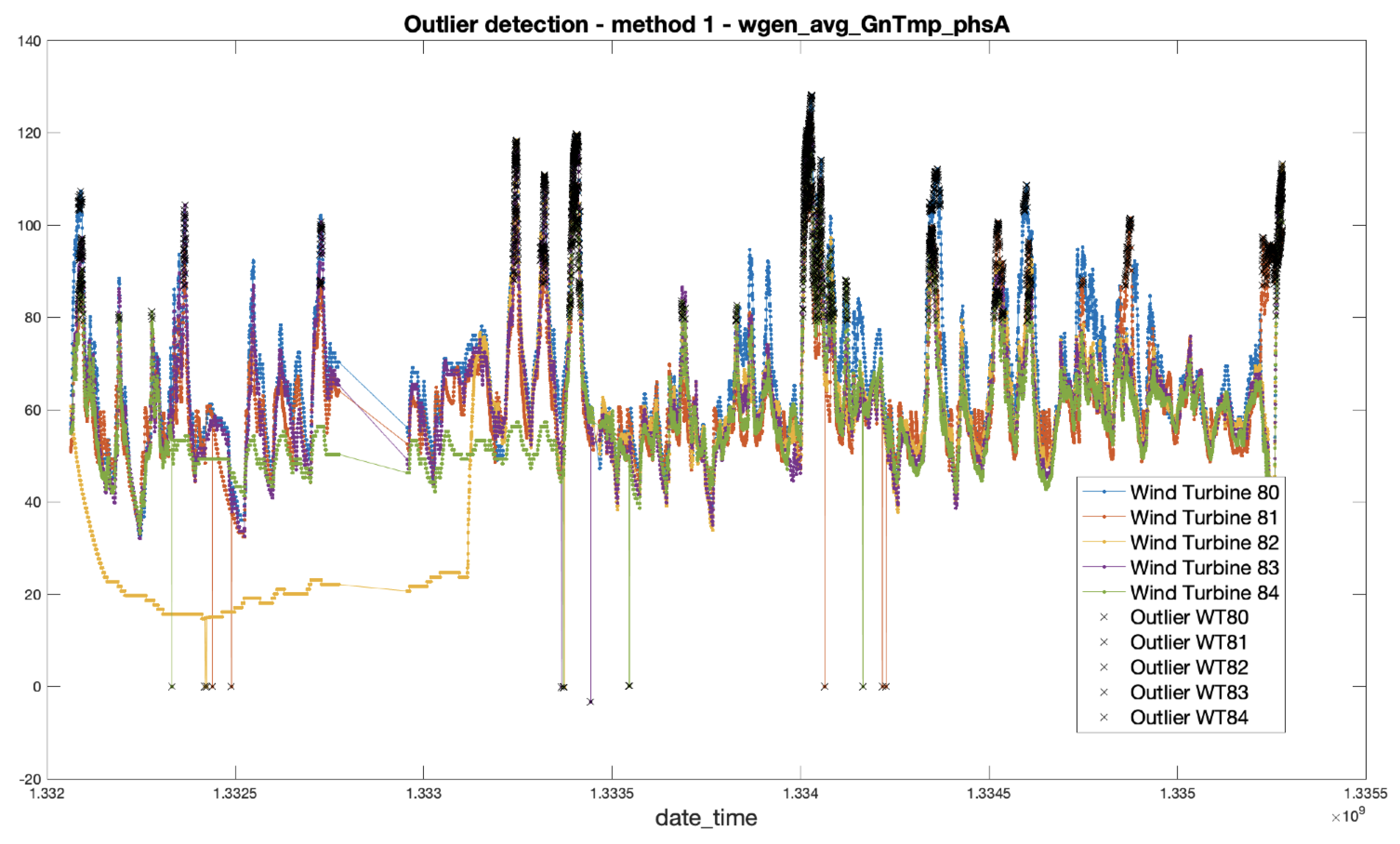
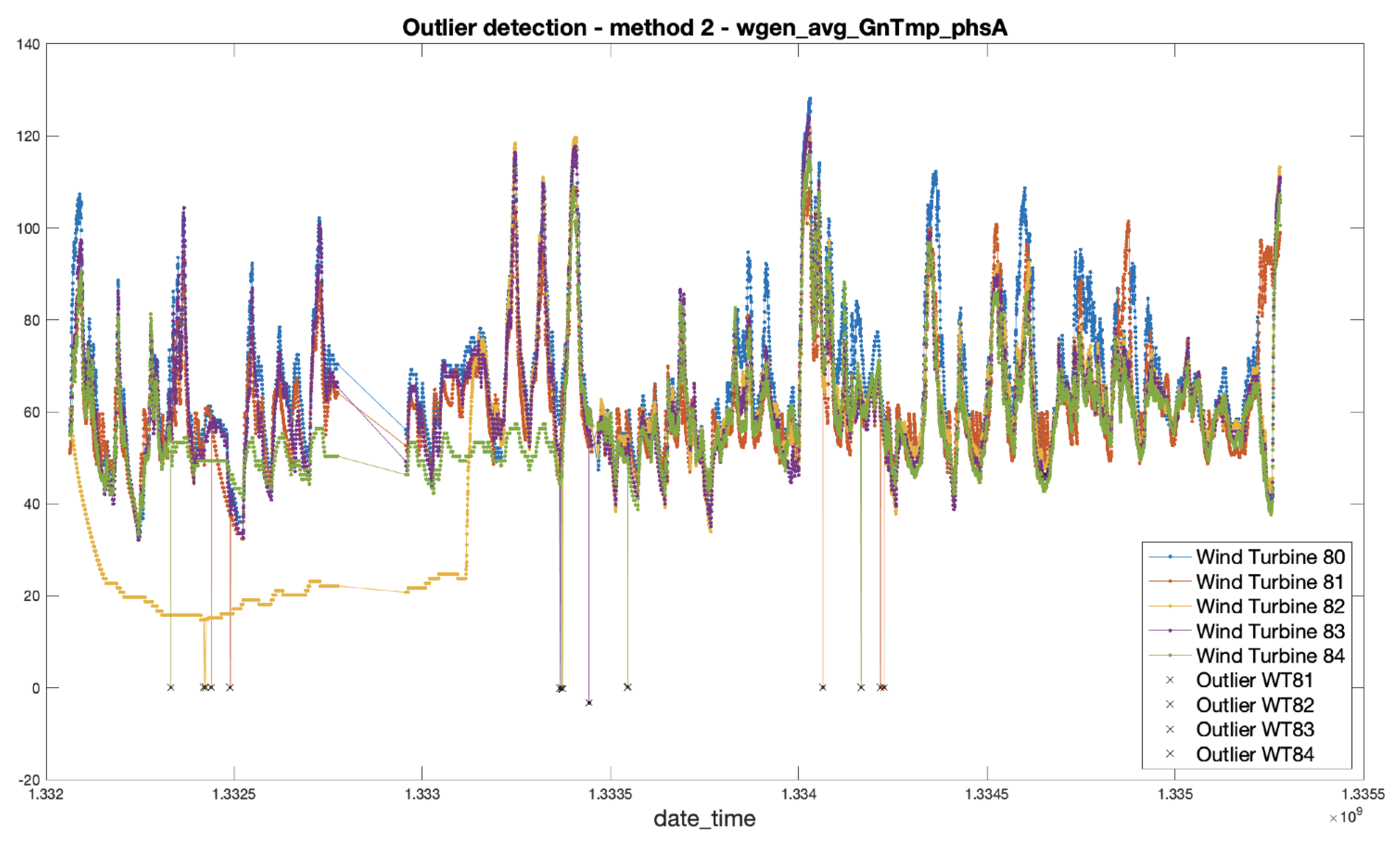
In the present work, only two configurations have been used: (i) the one applied to
Figure 2, which is widely used but does not work correctly in our problem, and (ii) the one applied to
Figure 3, which is taken as general, since it works very well on the whole set of available signals.
In this sense, the effect of using a typical filtering method consisting of eliminating values that exceed three times the scaled median absolute deviation (MAD) [
26] is shown in
Figure 2 The particularity of this filtering method is that it works on the entire signal. Let us consider that the samples are organized in the vector
. The scaled MAD is computed as
where the
represents the function that calculates the median of its input,
stands for the module, and
K is the scale factor taken by default as 1.4826 (the value taken when assuming Gaussian statistics). In this plot, in which the temperature
wgen_avg_GnTmp_phsA is depicted, it can be observed that the method captures values close to zero as outliers. The outliers are marked with a black cross. These detections are consistent with the laws of physics, as temperature values are subject to high inertia and cannot undergo such sharp variations. However, the method visibly fails when values corresponding to high amplitudes are removed, even though it is known that these values correspond to well-functioning states of the WT. After the application of this method, they would no longer be well represented.
Optimally, the filtering method for each signal should be determined according to the characteristics of each particular signal. For that, a method that works acceptably well for all recorded signals is proposed. It consists in determining that a value will be an outlier if it is more than 3.2 local standard deviations from the local mean calculated over a 25-sample moving window, which roughly correspond to 2 h of data. The fact of performing the operations on a moving window means that the filtering criteria are applied locally and not considering the whole range of values that the signal takes in the entire period of the recording. In
Figure 3, the points detected as outliers according to this second method are shown, for the same signals and period as those shown in
Figure 2. In this second case, the method does not clip the higher amplitude values of the signal. In order to generalise the process, this filter has been applied in the same way to all the signals.
3.4. Determination of the Reference Pattern of the Signal and the Residue
In this section, the reference pattern that the signal of each turbine follows is determined. This signal will be used as a reference to see how the signal of each turbine deviates from this standard by calculating the residual, i.e., the result of subtracting this reference from the signal of each turbine.
By calculating the pattern signal, it is assumed that most of the time the turbines work correctly and that it is highly improbable that more than half of the turbines fail simultaneously. Under this assumption, and for each
k point of the sequence, the pattern signal will be the median of the values of the 5 turbines at the point
k. More precisely, given the same signal of all WTs in the time instant
k, named
, the pattern
in
k is defined as
. Therefore, from now on, the pattern signal will be named as the median. In
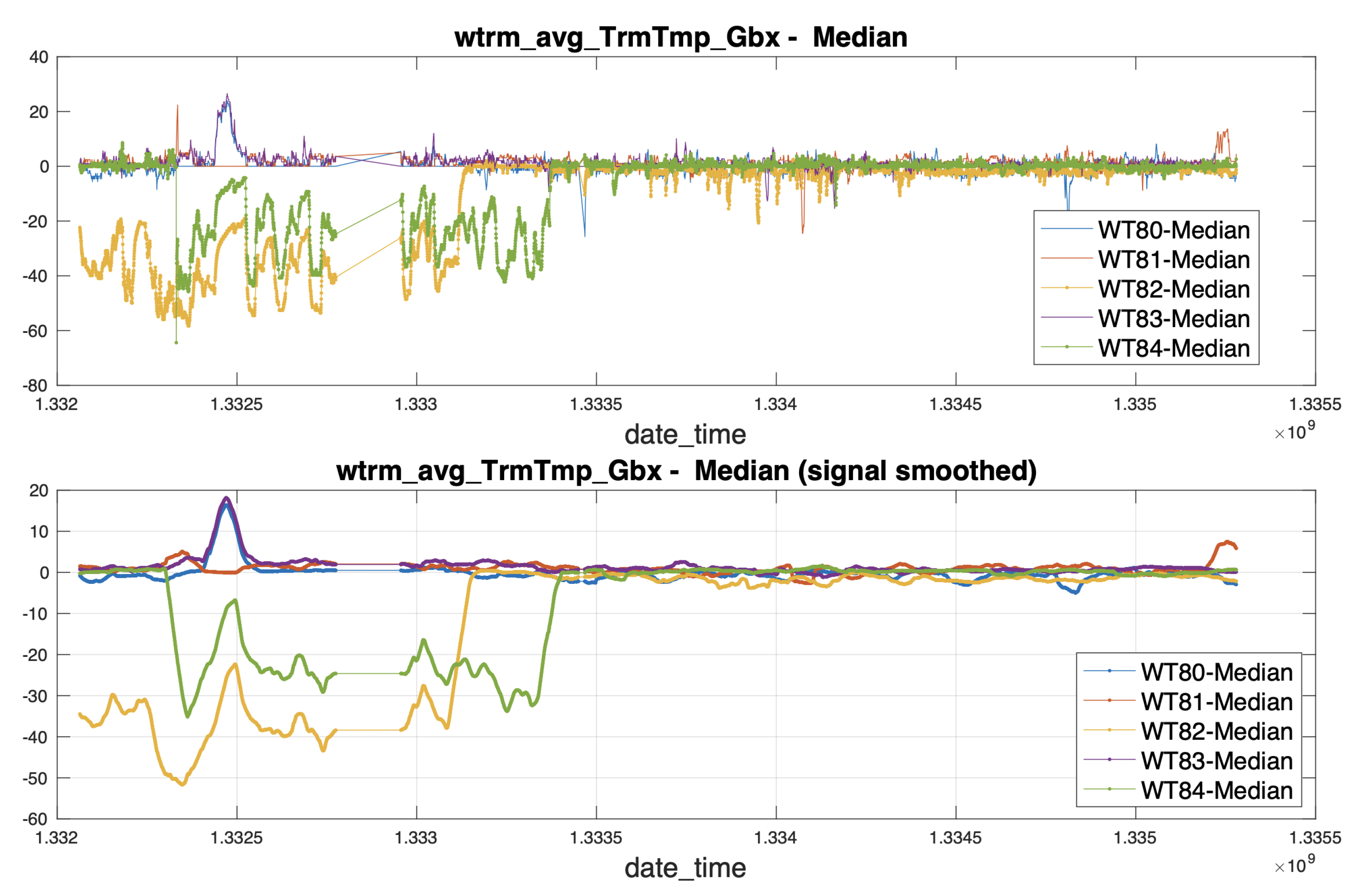
Figure 4, in the upper plot, the shape of the median over-imposed on the set of example signals is represented, and in the lower plot the residuals are represented. Note that the residuals of a well-functioning turbine stay or oscillate around zero or show sporadic peaks that return to the origin, but in the case of WT82 this residual diverges very perceptibly at the moment when it was stopped.
To improve the interpretation of the residuals, the signals can be smoothed by applying a moving average or a low-pass filter.
3.5. The Gearbox Subsystem
The gearbox system was chosen to carry out the experiments, following the work developed in [
4] and in a very similar way in [
27]. The gearbox is the part of the turbine that has the greatest impact on maintenance, repair, and manufacturing costs. As can be seen in Table 4 of NREL’s report [
28], the drivetrain, of which the gearbox is a part, is the second most expensive element to maintain, regardless of the way that amortised generation costs are calculated (CapEx & LCOE).
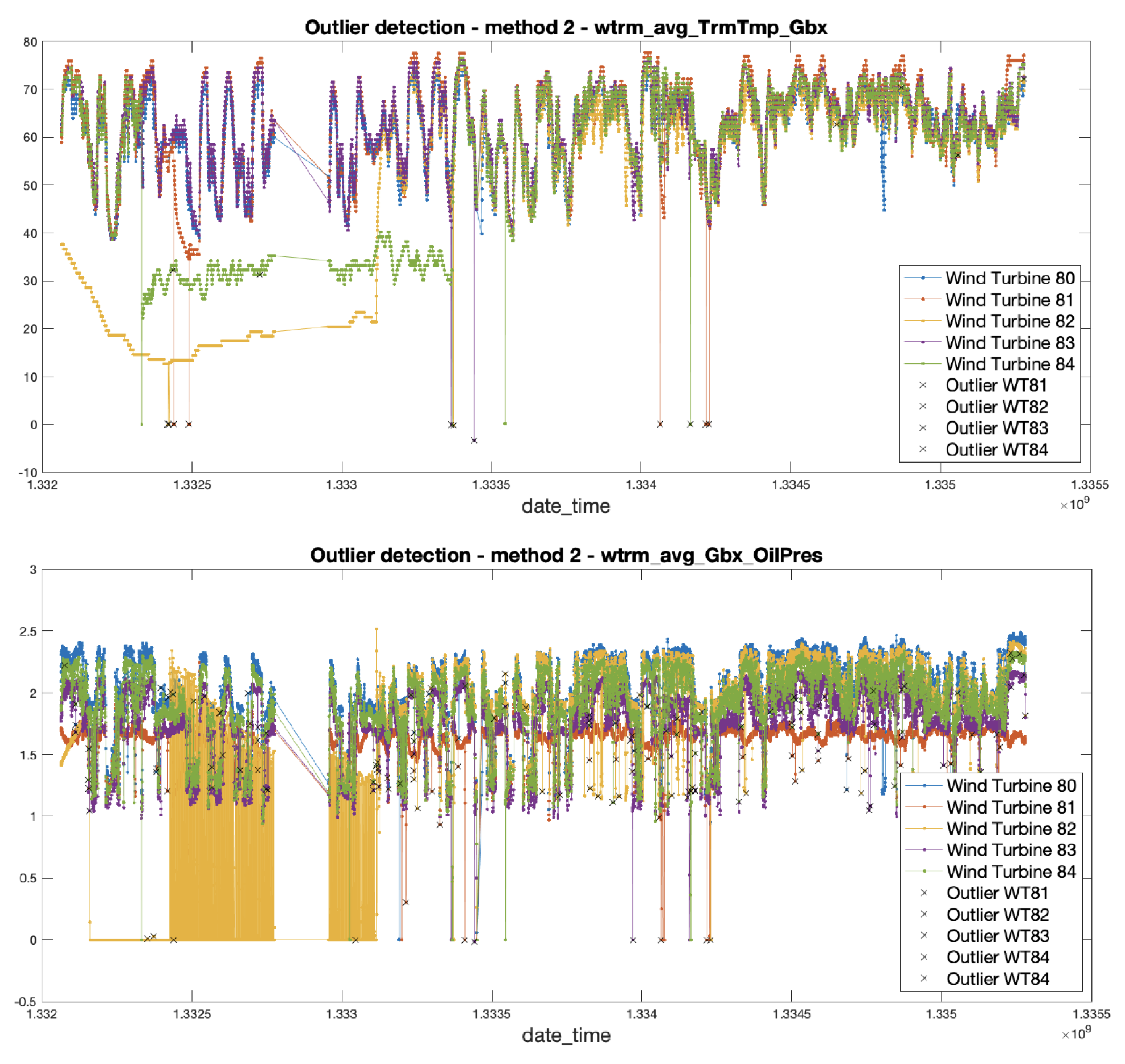
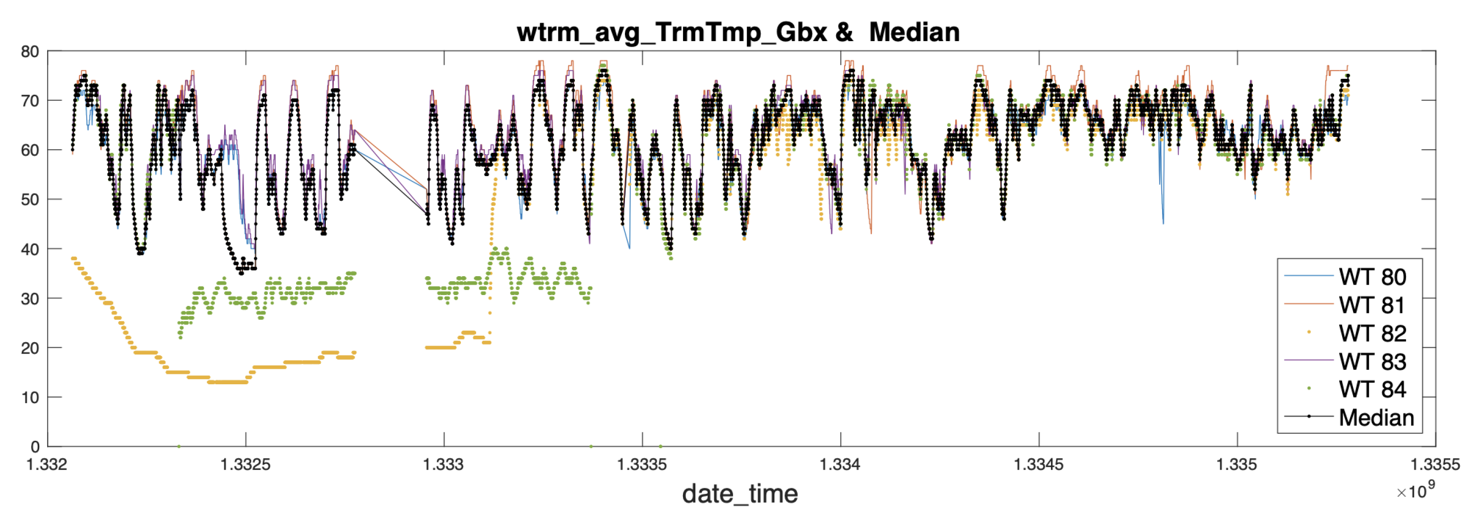
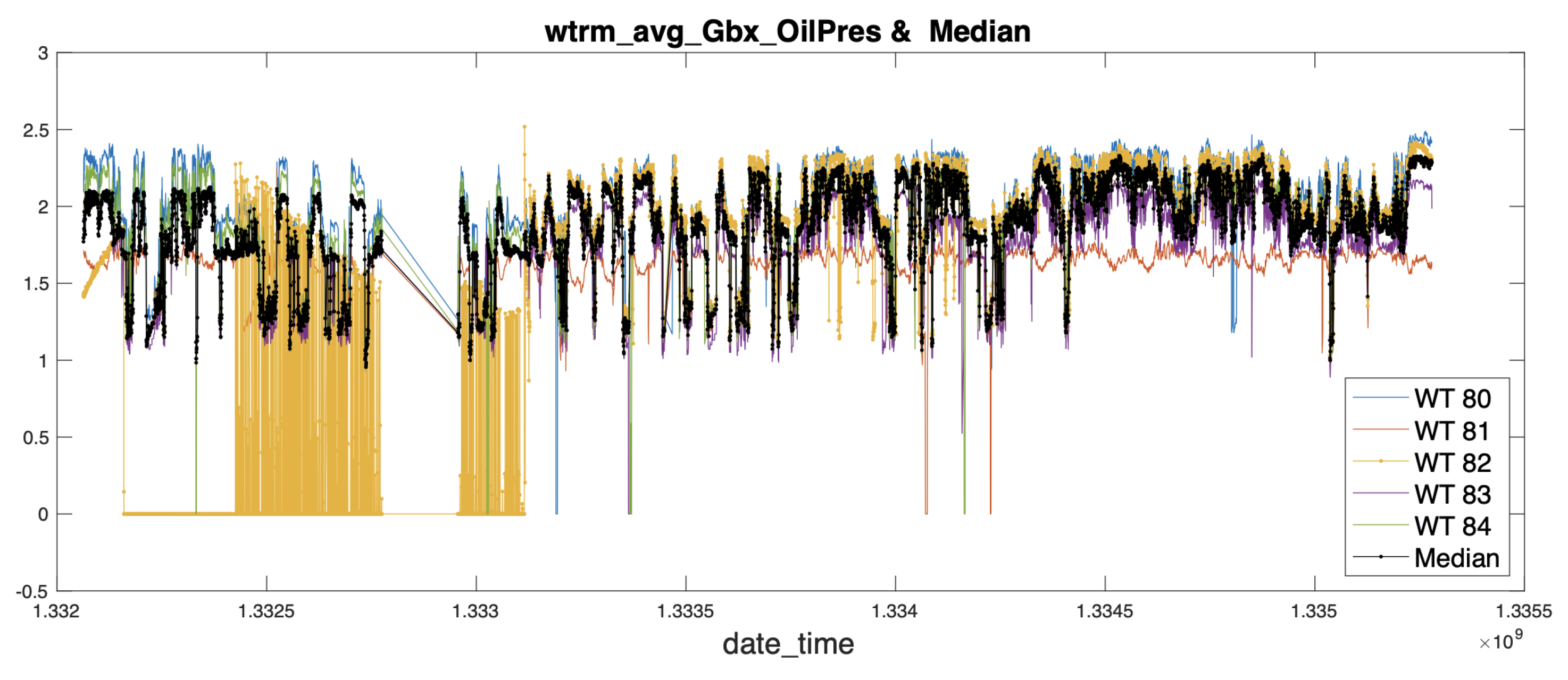
Given the importance of the prognosis of the gearbox subsystem, for its economic implications, two signals from this subsystem were selected to be analysed according to the procedure described above. To present the results, the experiments will focus on a temperature value and an oil pressure value. These are the signals
wtrm_avg_TrmTmp_Gbx and
wtrm_avg_Gbx_OilPress, which are represented in
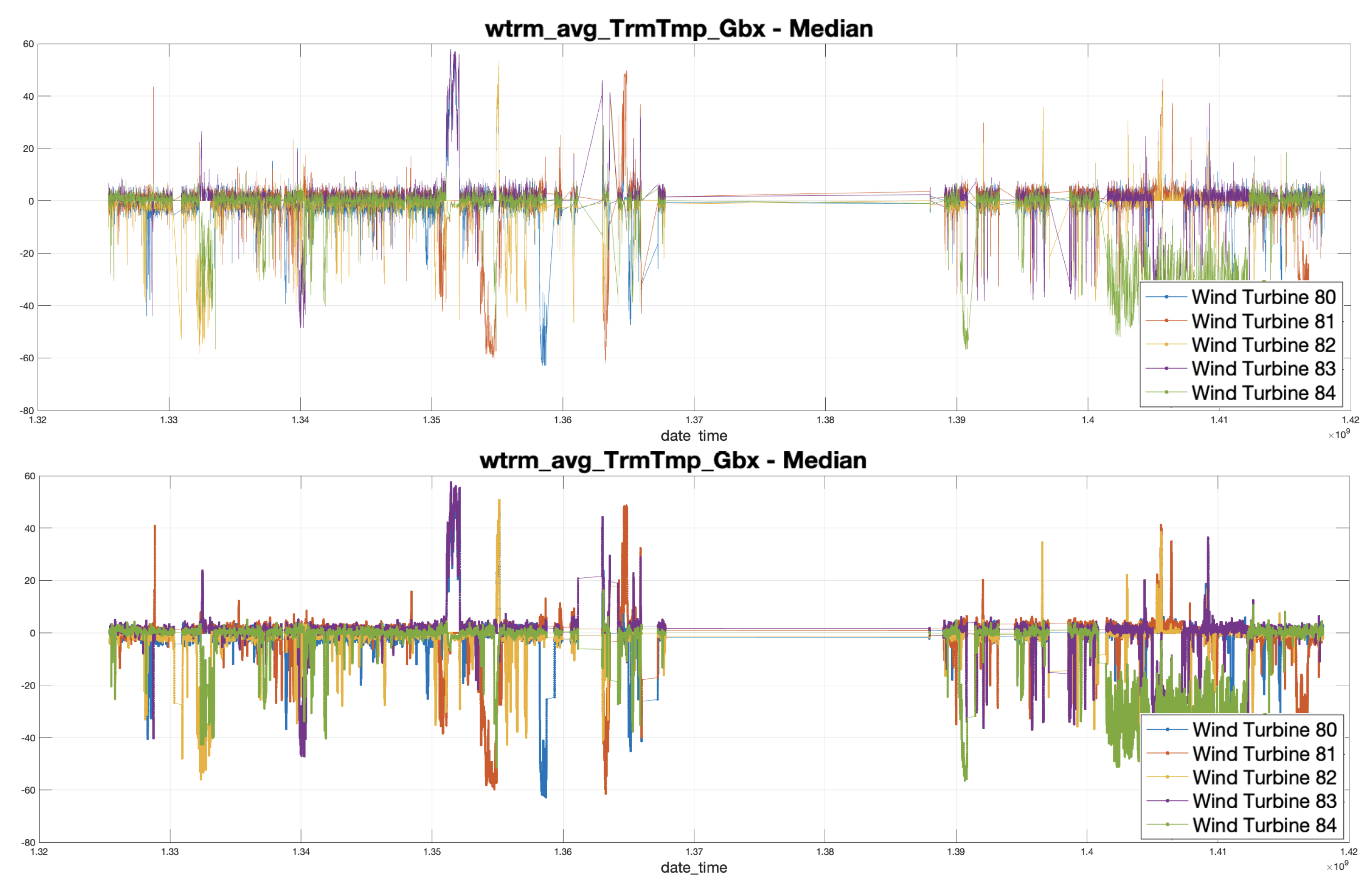
Figure 5. The time interval selected is the same used in the previous figures. Note also that the proposed outlier detection algorithm detects outliers generically, but some of them (marked with a cross in the figure) still remain.
For each of the two signals, the procedure carried out is detailed by means of plots. For the temperature signal,
wtrm_avg_TrmTmp_Gbx, in
Figure 6 the median and the signals are superimposed, while in
Figure 7 the residuals are depicted in the upper plot, while the smoothed residuals, using a 50-sample moving average filter, are depicted in the lower plot.
In
Figure 8, the median and the signals
wtrm_avg_Gbx_OilPress of each turbine are overlaid, while in
Figure 9 the residuals are depicted in the upper plot, while the smoothed residuals, using a 50-sample moving average filter, are depicted in the lower plot.
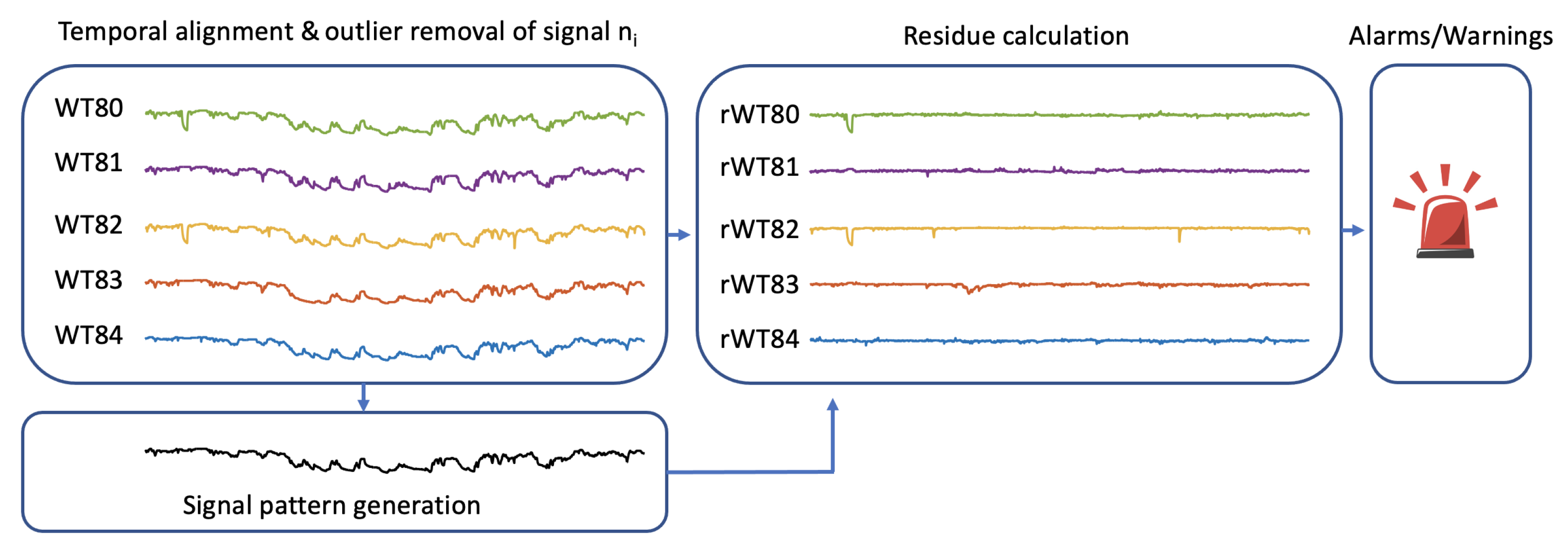
Figure 10 shows a simplified diagram of the proposed method. The first step consists of a time-strict alignment of the measurements of all the turbines and a preprocessing of outliers, performed on the basis of the temporal register that is incorporated into each measurement. To detect outliers, a conventional method is applied but evaluated in a time window. After this step, all measurements of the wind farm can be rearranged into a three-dimensional tensor that allows the simultaneous processing of all measurements. The reference pattern is calculated by simply taking the median of the same signals from each WT and applying it to each k-point. This reference signal is used to calculate the residuals of this signal for each WT by simply extracting the difference between the reference and the actual signal at each WT.
Figure 10, for a single signal, depicts this idea. From the analysis and tracking of the residuals, alarms are generated in the same way as they are generated in a regression-based ML model.
The mathematics of this process are fairly straightforward. It involves calculating the means to find the reference signal, subtractions to find the residuals, and moving averages, both to smooth the residuals and to detect outliers. Let us now summarise them.
The median of dataset
of
n values,
, is computed by first ordering the values of this data set from smallest to largest such that the smallest is
and the largest is
; then, depending on whether
n is even or odd, one has:
To perform the smoothing of the signal
, a simple moving average (SMA) filter with a temporal window of N samples is used, according to the following expression:
which can be effectively computed by the following recursive form:
One way to interpret the smoothing is to determine the Discrete Fourier Transform (DFT) of the filter through the study of the Z transform of any of the expressions (
2) or (
3):
When replacing
z by
in (
4), and performing some operations, the DFT is obtained, in terms of the discrete frequency
, which is:
Note that N, the length of the moving window, controls the pass-band of this simple low-pass filter, so that the larger the N, the narrower the pass-band.
Finally, note that the same moving average filter has been used to filter outliers. The samples within the temporal moving window are used to calculate the standard deviation when the filter is used for this purpose. Then, if , will be labelled as an outlier.
4. Results
In this section, two signals from the gearbox subsystem are processed using the proposed method and all the data available in the database. These are the temperature signal
wtrm_avg_TrmTmp_Gbx and the pressure signal
wtrm_avg_Gbx_OilPress shown in the previous section. In
Figure 11 the residuals obtained from
wtrm_avgg_TrmTmp_Gbx in each of the five turbines are overlaid. In the upper plot, the raw residuals are shown, while in the lower plot they are shown after being filtered with a 50-sample moving average filter, which makes the interpretation easier. In
Figure 12, the same representation is available for the residuals of the
wtrm signal. These two plots, due to the overlapping of the signals and the long time interval covered, are difficult to interpret but they allow us to notice the relative amplitudes and peaks that appear occasionally in the different turbines, and show that at some point these signals separate from the signal that was defined as a reference from the median.
To improve the interpretation of these results, in the following figures we separate the information of these two graphs by turbines and compare them with the rotor speed,
wgen_avg_RtrSpd_IGR.
Figure 13,
Figure 14,
Figure 15,
Figure 16 and
Figure 17 show the information for turbines WT80, WT81, WT82, WT83, and WT84, respectively. For each of these plots, in the central part the signal
wgen_avg_RtrSpd_IGR in the colour used to identify the turbine, is plotted. In the upper part, in black, the residue is coming from
wtrm_avg_Gbx_OilPress, but it is reversed, so that the positive peaks of the
Figure 12, in this representation, point downwards. The lower signal, also in black, represents the smoothed residual of the temperature signal, without any inversion. In the set of these five plots, the signals are scaled for a pleasing display, so their absolute amplitudes do not provide information. The information is in the position of the peaks of the residuals, their relative amplitude, and their position in relation to the sections where the turbine shows speed values of the
wgen_avg_RtrSpd_IGR in the vicinity of zero. The rotor speed has the particularity that it allows to identify when a turbine is inactive while the rest of the turbines are working, which is indicative that the turbine is stopped, either in maintenance phase, or presumably out of order, and therefore in repair phase.
In other words, when there is sufficient wind to move the set of turbines, the
wgen_avg_RtrSpd_IGR signals of the turbines follow the operating pattern. However, if one WT is stopped, its
wgen_avgen_avgg_RtrSpdSpd_IGR is measured as zero, decoupling it from the general pattern. A detailed example can be seen in the last plot of
Figure 1, where the signal
wgen_avg_RtrSpdd_IGR corresponding to the WT82 (in yellow), becomes zero when the rest of the signals of the same turbine (also in yellow) and represented in the upper plots, uncouple from the pattern.
In
Figure 13,
Figure 14,
Figure 15,
Figure 16 and
Figure 17, the periods in which a turbine is stopped are represented in those intervals where the central signal is zero. The blue rectangles added in these figures (11 in total) highlight the time intervals where a peak in the residuals (black signals) is detected and the WT is stopped. The red rectangles (two in total, one in
Figure 13 and one in
Figure 17) show the presence of peaks in the residuals, but in this case the turbine is not stopped.
In each of these plots there are blue rectangles that mark areas where there is a peak in some residue signal and capture a section where the rotor speed is zero and therefore the turbine is stopped. When that is the case, it can be noticed—but not always—that in both residues a peak is produced simultaneously. Note that there are few peaks of significant width that are not accompanied by the section, indicating that the turbine has stopped, although one can be found at the beginning of the
Figure 17 corresponding to the WT84.
In
Figure 13 and
Figure 16, the presence of a red rectangle can be observed, indicating that despite the occurrence of important peaks, the turbines WT80 and WT83 do not stop. In this case, we note that the peaks occur at the same time instants on both turbines. Moreover, at the same instant time, the other three WTs (81, 82, and 84) also present peaks, indicating that the turbines stopped, and in these three turbines, it is indeed registered as a stop. In this case, the presence of the peaks in all the turbines is precisely due to the simultaneous stop of the three of them, more than half of the turbines, which causes the median filter to select, as a reference signal, the samples corresponding to one of the machines that is stopped, which ends up in the centrality position.
5. Discussion
Although the database has been exploited previously in other work to derive different normality models for the exploration of different subsystems, this technique uncovered subsets of data that were used in the training part of the model, but were mislabelled, i.e., used in the wrong class. While this is a relatively small proportion of the data, retraining the models with the more correctly labelled training data would provide a slight overall improvement in model performance. The strategy employed was to use the first half of the data for training, and although all machines had small stops in this time frame, some of these had not been detected.
Thanks to the proposed method, if a turbine in the wind farm fails, the specific location of the failure can be determined as follows: Typically, WTs are analysed by subsystems. This means analysing the set of signals segregated into smaller groups according to the part of the WT they belong to. This allows faults to be isolated. Let us say, for example, that subsystem A is analysed and the failure occurs on subsystem B. What is observed in the signals belonging to subsystem A is that, if the failure is important enough to stop the WT, at the moments when the WT is stopped, peaks appear in the residuals and, obviously, if the WT is stopped, the rotor speed, the instantaneous power produced, etc., records are zero. In this sense, failure is not anticipated, but a way to automatically isolate the time windows in which the WT stops is obtained, which allows segmenting or correctly labelling sections of data to improve the training phase of the supervised models. In a context where wind farms have many WTs (more than a hundred, in many cases) and because each WT has hundreds of measurements recorded continuously for many years, applying this technique can be very helpful. It is even more interesting, however, when the failure occurs in the signals of the system under analysis. In that case, if the failure is caused by the progressive deterioration of some mechanism, the signals involved begin to vary the pattern gradually and the failure can be anticipated. This occurs in
Figure 17, corresponding to the analysis of the WT84. This failure affected the gearbox. The largest blue square selects the time interval where the WT failed. Here it is interesting to note that the peaks of the residuals, generated from signals from this subsystem, start to appear before the WT stops (zero-valued section in the central green signal).
A brief analysis of the results found shows that they are consistent with what was observed in previous analyses of this area. The tests were carried out with the second part of the data of the turbines. As it is also reflected in the residue analysis, the first three turbines, WT80 (
Figure 13), WT81 (
Figure 14), and WT82 (
Figure 15) have better health than the previous ones. The best of all is WT82 (
Figure 15), which does not present any problem during the test period. The turbines WT81 and WT82 only have one problem that leaves them inactive for a short time. The turbine WT83 (
Figure 16), also with a single problem in the test part, remained inoperative for a considerably longer period of time. Finally, it should be noted that the WT84 turbine (
Figure 17) was inoperative due to a problem in the gearbox that left it inactive for much longer than the rest, as the repair of this subsystem, in addition to being economically costly, is slow. We note that the analysed signals,
wtrm_avg_TrmTmp_Gbx and
wtrm_avg_Gbx_OilPress belong to this subsystem. In this context, it is observed that the peak in the residue from the
wtrm_avg_TrmTmp_Gbx in the blue rectangle anticipates the failure. Additionally, we note that a peak had previously been generated in the two residues (
wtrm_avg_TrmTmp_Gbx and
wtrm_avg_Gbx_OilPress), which did not cause any stop but could possibly anticipate a problem in this subsystem.
6. Conclusions
The set of SCADA variables of all the turbines in the wind-farm operating correctly follows a well-defined variation pattern group, especially by the variables of the type _avg. When one of the turbines malfunctions, or stops working, its variable set is decoupled from the general pattern. These two facts allow a comparison of the health status of the turbines. To do the comparison, a reference signal is calculated, corresponding to the median value of the signals of each turbine. The underline idea is that WTs will hardly fail all at the same time, so that the detection of the malfunction of one of them can easily be done via the difference of their signals with the reference signal. In this first exploration it can be seen that the residuals, the difference between the signal from each turbine and the reference signal, have an interesting and powerful potential to generate warnings and that most of them are related to the status of the wind turbine. Moreover, the detection of a fault does not only appear in the signals associated with the subsystem that fails, but also transversely in the rest of the variables in a very general way. Hence, the detection of abnormal behaviour does not depend on the exploration of a single signal.
An advantage of the presented technique is its explainability, as we can see why the peaks are generated in the residue. In the present format, the representation of the signals can already provide a visual idea of the occurrence of potential problems. In fact, an analyst can study and interpret the signals causing the alarm and assessing the risk before a failure.
Another advantage is that once the strict time alignment of all the data of all the signals of all the WTs has been verified, the information can be stored in tensors (multidimensional matrices), which can be of third order, where the dimensions can be time × signals × WT. The operations involved, such as filtering outliers, can be performed very quickly on this structure. Similarly, reference signals or patterns can be calculated by performing the variance operation, operating only in the third dimension of the tensor. This means that with very simple operations, the residuals of all the signals of interest of an entire park can be generated massively and automatically without the need to train models. Compared to supervised systems, this is a very important advantage. This method could also be easily modified and used to mark the signal sections where WTs are stopped to better refine the signal sets that are selected.This would allow better labelling of the signals used in the training phase, e.g., by discarding the sections where WT stops, if one wants to train a normality model for the forecast. It should be noted that the strategy presented is simple and allows a massive analysis of all the signals, being easily parallelised and with a very controlled computational cost.
However, as with all methods, the proposed method has some possible drawbacks. One of the disadvantages is the need to introduce a threshold on the residual signal when generating alarms automatically. This disadvantage is common with the normality models based on regressors that also need to apply a threshold on the error signal when generating an alarm automatically. At this point, operator supervision would be desirable. In the work presented, there have been a total of 13 possible alarms (the rectangles in
Figure 12,
Figure 13,
Figure 14,
Figure 15 and
Figure 16) over an interval of almost 2 years, which represents an easily manageable volume. Another disadvantage in presenting this paper is that it is a seminal work and there are no other works on systems using SCADA signals with information from various WTs in the wind farm available for comparison. It will therefore be interesting for future work on other data to use the proposed method and confirm its effectiveness.
