
Stride-TCN for Energy Consumption Forecasting and Its Optimization

 , ,
, , 
Abstract
:1. Introduction
- -
- We propose a new TCN architecture with performance on par with state-of-the-art models on several benchmarks, but the number of parameters is greatly reduced based on the stride mechanism. We search for the best stride hyperparameter, representing cyclic patterns on the data.
- -
- We introduce a dataset of electrical energy consumption measured at Chonnam National University (CNU), South Korea. Along with the dataset, we also present the baseline benchmark.
2. Background
3. Methodology
3.1. Time Series Forecasting Problem
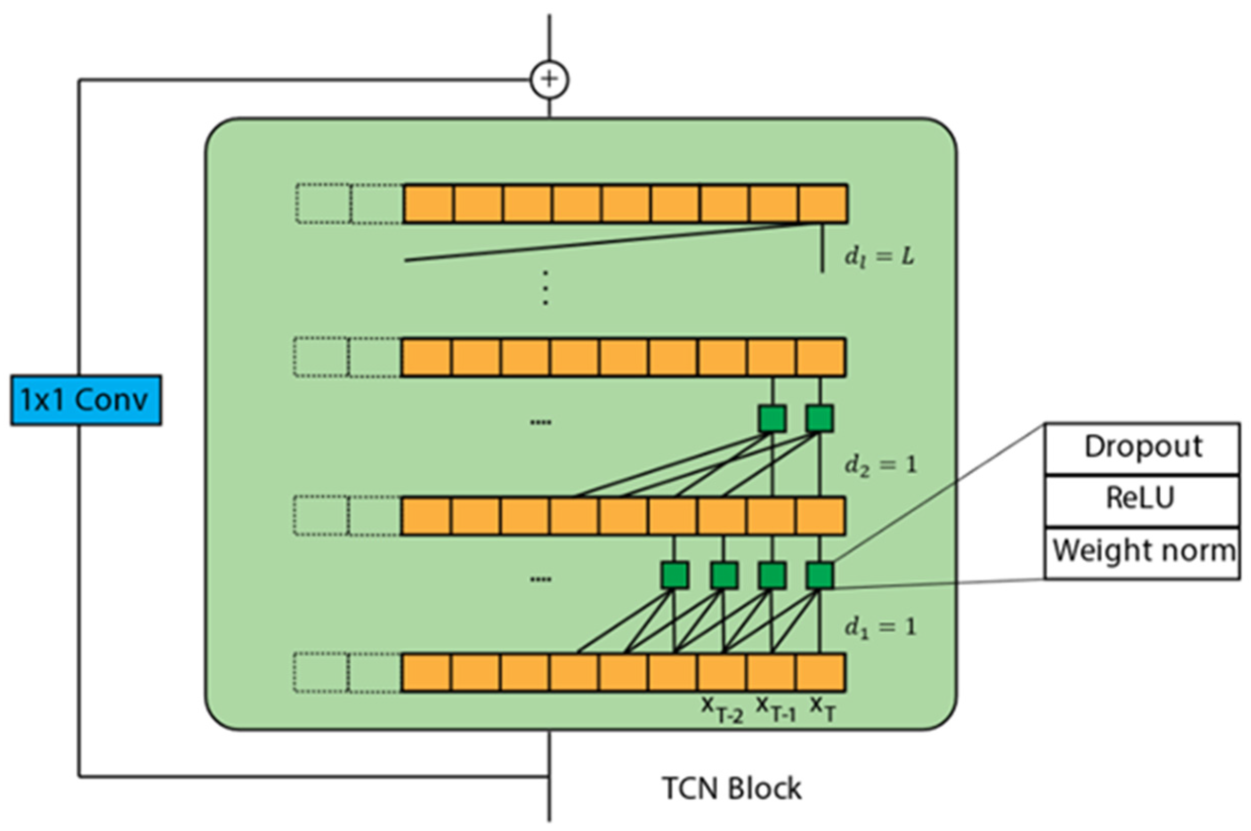
3.2. TCN Architecture
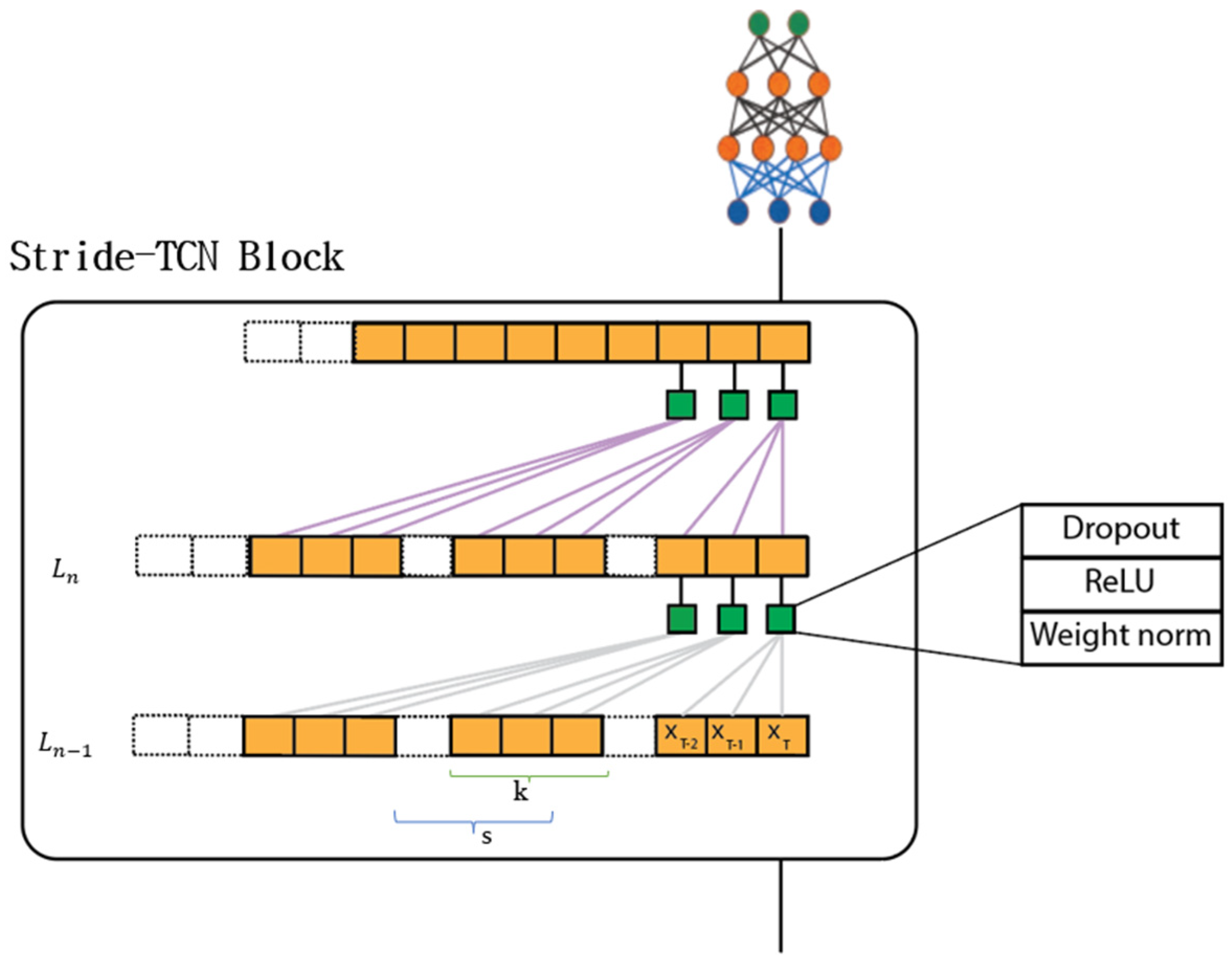
3.3. Stride-TCN
3.4. Bayesian Optimization
| Algorithm 1 Bayesian Optimization (BO) |
| Input: Search space , black-box function F, acquisition function , maximal number of function evaluations 1. = initialize() 2. for n = 1 to do 3. = fit predictive model on ; 4. select by optimizing 5. end for 6. Query 7. Add observation to data ; 8. return Best |
3.5. Training Procedure
| Algorithm 2 Training procedure |
| Input: Search space epoch = 100; 1. Algorithm 1 () 2. Initialize W with 3. for n = 1 to epoch do 4. Update W based on Huber loss (W) 5. end for |
4. Experiments
4.1. Setup
4.1.1. Datasets
4.1.2. Model variants
4.1.3. Evaluation Metrics
4.2. Experimental Results and Comparison
4.2.1. Baselines and Configurations
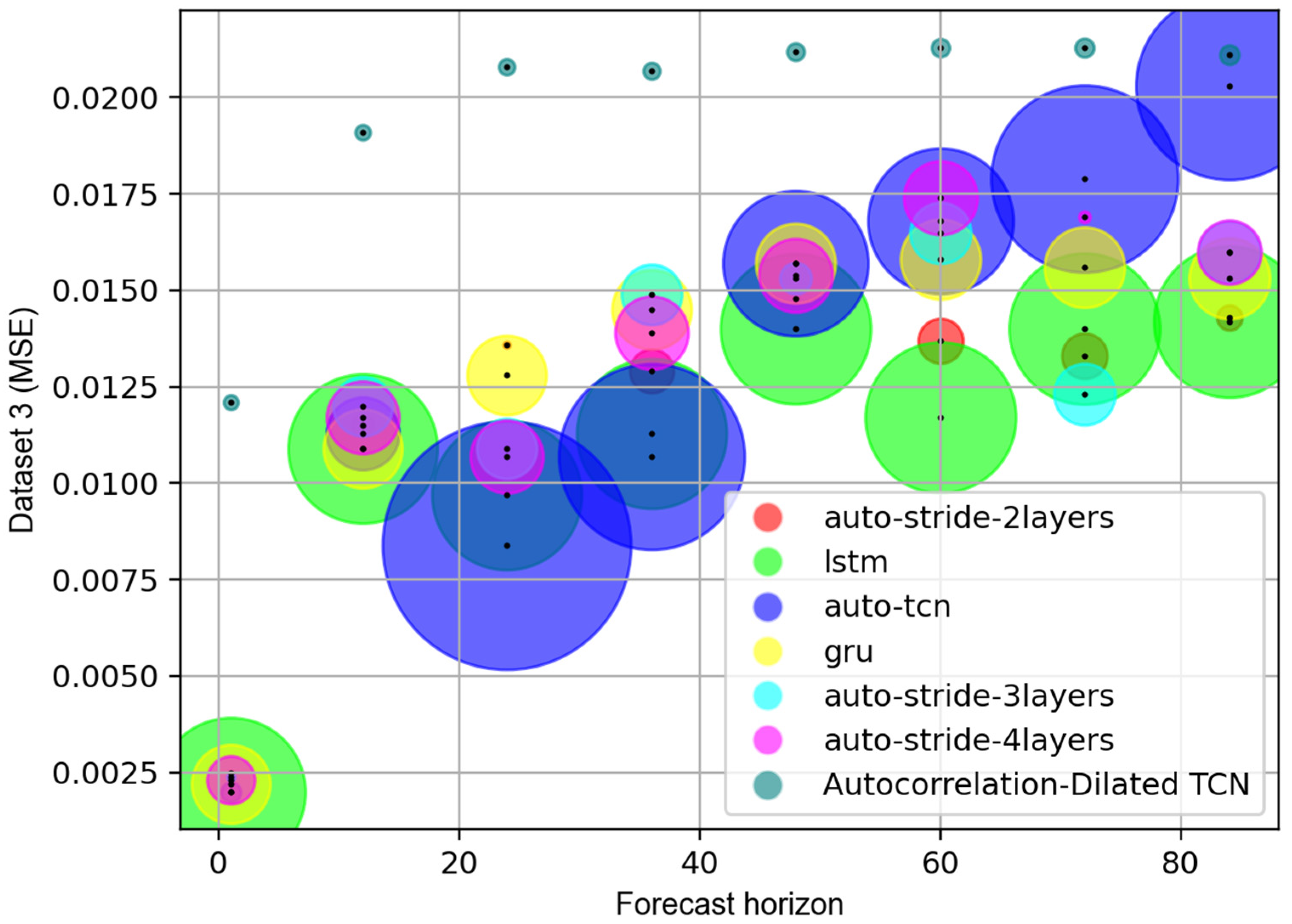
4.2.2. Results and Analysis
5. Conclusions
Author Contributions
Funding
Institutional Review Board Statement
Informed Consent Statement
Data Availability Statement
Conflicts of Interest
References
- Akaike, H. Fitting autoregressive models for prediction. Ann. Inst. Stat. Math. 1969, 21, 243–247. [Google Scholar] [CrossRef]
- Frigola, F.; Rasmussen, C.E. Integrated pre-processing for Bayesian nonlinear system identification with Gaussian processes. In Proceedings of the 52nd IEEE Conference on Decision and Control, Firenze, Italy, 10–13 December 2013; pp. 552–560. [Google Scholar]
- Shi, J.; Jain, M.; Narasimhan, G. Time Series Forecasting (TSF) Using Various Deep Learning Models. arXiv 2022, arXiv:2204.11115. [Google Scholar]
- Jadon, S.; Milczek, J.K.; Patankar, A. Challenges and approaches to time-series forecasting in data center telemetry: A Survey. arXiv 2021, arXiv:2101.04224. [Google Scholar]
- Nelson, B.K. Time series analysis using autoregressive integrated moving average (ARIMA) models. Acad. Emerg. Med. 1998, 5, 739–744. [Google Scholar] [CrossRef] [PubMed]
- Rousseeuw, P.J.; Hampel, F.R.; Ronchetti, E.M.; Stahel, W.A. Robust Statistics: The Approach Based on Influence Functions; John Wiley & Sons: Hoboken, NJ, USA, 2011. [Google Scholar]
- Bai, S.; Kolter, J.Z.; Koltun, V. An empirical evaluation of generic convolutional and recurrent networks for sequence modeling. arXiv 2018, arXiv:1803.01271. [Google Scholar]
- Gan, Z.; Li, C.; Zhou, J.; Tang, G. Temporal convolutional networks interval prediction model for wind speed forecasting. Electr. Power Syst. Res. 2021, 191, 106865. [Google Scholar] [CrossRef]
- Li, D.; Jiang, F.; Chen, M.; Qian, T. Multi-step-ahead wind speed forecasting based on a hybrid decomposition method and temporal convolutional networks. Energy 2022, 238, 121981. [Google Scholar] [CrossRef]
- Cao, Y.; Ding, Y.; Jia, M.; Tian, R. A novel temporal convolutional network with residual self-attention mechanism for remaining useful life prediction of rolling bearings. Reliab. Eng. Syst. Saf. 2021, 215, 107813. [Google Scholar] [CrossRef]
- Singhania, D.; Rahaman, R.; Yao, A. Coarse to Fine Multi-Resolution Temporal Convolutional Network. arXiv 2021, arXiv:2105.10859. [Google Scholar]
- Pingchuan, M.; Yujiang, W.; Jie, S.; Stavros, P.; Maja, P. Lip-Reading With Densely Connected Temporal Convolutional Networks. In Proceedings of the IEEE/CVF Winter Conference on Applications of Computer Vision (WACV); 2021. Available online: https://openaccess.thecvf.com/content/WACV2021/html/Ma_Lip-Reading_With_Densely_Connected_Temporal_Convolutional_Networks_WACV_2021_paper.html (accessed on 4 August 2022).
- Oord, A.; Dieleman, S.; Zen, H.; Simonyan, K.; Vinyals, O.; Graves, A.; Kalchbrenner, N.; Senior, A.; Kavukcuoglu, K. Wavenet: A generative model for raw audio. arXiv 2016, arXiv:1609.03499. [Google Scholar]
- Churchill, R.M.; Tobias, B.; Zhu, Y.; DIII-D Team. Deep convolutional neural networks for multi-scale time-series classification and application to tokamak disruption prediction using raw, high temporal resolution diagnostic data. Phys. Plasmas 2020, 27, 062510. [Google Scholar] [CrossRef]
- Broersen, P.M. Automatic Autocorrelation and Spectral Analysis; Springer Science & Business Media: New York, NY, USA, 2006. [Google Scholar]
- Dewancker, I.; McCourt, M.; Clark, S. Bayesian Optimization Primer; 2015. Available online: https://app.sigopt.com/static/pdf/SigOpt_Bayesian_Optimization_Primer.pdf (accessed on 15 September 2022).
- Jones, D.R.; Schonlau, M.; Welch, W.J. Efficient global optimization of expensive black-box functions. J. Glob. Optim. 1998, 13, 455–492. [Google Scholar] [CrossRef]
- Lindauer, M.; Feurer, M.; Eggensperger, K.; Biedenkapp, A.; Hutter, F. Towards Assessing the Impact of Bayesian Optimization’s Own Hyperparameters. In Proceedings of the IJCAI 2019 DSO Workshop, Macao, China, 10–16 August 2019. [Google Scholar]
- Parate, A.; Bholte, S. Individual household electric power consumption forecasting using machine learning algorithms. Int. J. Comput. Appl. Technol. Res. 2019. Available online: https://www.researchgate.net/publication/335911657_Individual_Household_Electric_Power_Consumption_Forecasting_using_Machine_Learning_Algorithms- (accessed on 7 July 2022). [CrossRef]


| Hyperparameters | Symbol | Choices |
|---|---|---|
| 1D convolutional window size | 1, 3, 5, 7, 9 | |
| Number of filters in each convolution layer | 8, 16, 32, 64, 128, 256, 512 | |
| Number of TCN layers | ||
| Dilation factor | ||
| Skip connection | Yes, No | |
| Batch Normalization | Yes, No |
| Hyperparameters | Symbol | Choices |
|---|---|---|
| Kernal size | 1, 3, 5, 7, 9 | |
| Number of filters | 8, 16, 32, 64, 128, 256, 512 | |
| Stride | ||
| Dropout rate | 0, 0.1,…0.5 |
| Datasets | Length of Time Series | Total Number of Variables | Attributions |
|---|---|---|---|
| Dataset 1 | 2,075,259 | 7 | Global active power |
| Global reactive power | |||
| Voltage | |||
| Global intensity | |||
| Submetering 1 | |||
| Submetering 2 | |||
| Submetering 3 | |||
| Dataset 2 | 8760 | 2 | Energy consumption |
| Outside temperature | |||
| Dataset 3 | 11,232 | 1 | Energy consumption |
| Hyperparameters | Dataset 1 | Dataset 2 | Dataset 3 |
|---|---|---|---|
| 1D convolutional window size | 3 | 3 | 3 |
| Number of filters in each convolution layer | 32 | 32 | 32 |
| Stride 1 | 12 | 24 | 24 |
| Stride 2 | 7 | 7 | 7 |
| Method | Time Prediction | |||||||||||||||
|---|---|---|---|---|---|---|---|---|---|---|---|---|---|---|---|---|
| 1 h | 12 h | 24 h | 36 h | 48 h | 60 h | 72 h | 84 h | |||||||||
| MSE | MAE | MSE | MAE | MSE | MAE | MSE | MAE | MSE | MAE | MSE | MAE | MSE | MAE | MSE | MAE | |
| LSTM | 0.0020 | 0.0297 | 0.0109 | 0.0687 | 0.0097 | 0.0670 | 0.0113 | 0.0741 | 0.0140 | 0.0813 | 0.014 | 0.083 | 0.0140 | 0.0830 | 0.0145 | 0.0861 |
| GRU | 0.0022 | 0.0309 | 0.0109 | 0.0702 | 0.0128 | 0.0764 | 0.0145 | 0.0818 | 0.0157 | 0.0853 | 0.0156 | 0.0866 | 0.0156 | 0.0866 | 0.0153 | 0.0871 |
| TCN | 0.0020 | 0.0298 | 0.0113 | 0.0718 | 0.0084 | 0.0639 | 0.0107 | 0.0714 | 0.0157 | 0.0852 | 0.0168 | 0.0886 | 0.0179 | 0.0927 | 0.0203 | 0.0980 |
| Heuristic–stride–TCN | 0.0121 | 0.0799 | 0.0191 | 0.1012 | 0.0208 | 0.1049 | 0.0207 | 0.1044 | 0.0212 | 0.105 | 0.0213 | 0.1053 | 0.0213 | 0.1053 | 0.0211 | 0.1047 |
| Stride–TCN | ||||||||||||||||
| 2 layers | 0.0025 | 0.034 | 0.0115 | 0.0763 | 0.0136 | 0.0795 | 0.0129 | 0.0793 | 0.0148 | 0.0843 | 0.0137 | 0.0823 | 0.0133 | 0.0793 | 0.0142 | 0.0849 |
| 3 layers | 0.0024 | 0.0331 | 0.012 | 0.0725 | 0.0109 | 0.071 | 0.0149 | 0.0837 | 0.0153 | 0.0841 | 0.0165 | 0.0865 | 0.0123 | 0.0771 | 0.016 | 0.0868 |
| 4 layers | 0.0023 | 0.0322 | 0.0117 | 0.0765 | 0.0107 | 0.0727 | 0.0139 | 0.0833 | 0.0154 | 0.0828 | 0.0174 | 0.0922 | 0.0169 | 0.0888 | 0.016 | 0.0865 |
| Method | Time Prediction | |||||||||||||||
|---|---|---|---|---|---|---|---|---|---|---|---|---|---|---|---|---|
| 1 h | 12 h | 24 h | 36 h | 48 h | 60 h | 72 h | 84 h | |||||||||
| MSE | MAE | MSE | MAE | MSE | MAE | MSE | MAE | MSE | MAE | MSE | MAE | MSE | MAE | MSE | MAE | |
| LSTM | 0.0081 | 0.0677 | 0.0169 | 0.0971 | 0.0165 | 0.096 | 0.0169 | 0.0974 | 0.016 | 0.0949 | 0.0173 | 0.0982 | 0.0158 | 0.0949 | 0.0163 | 0.0957 |
| GRU | 0.0095 | 0.0723 | 0.0161 | 0.0937 | 0.0167 | 0.0955 | 0.0188 | 0.1015 | 0.0197 | 0.1037 | 0.02 | 0.1044 | 0.0198 | 0.104 | 0.0205 | 0.1061 |
| TCN | 0.008 | 0.0672 | 0.0149 | 0.0894 | 0.0156 | 0.0921 | 0.0166 | 0.096 | 0.0173 | 0.0981 | 0.0187 | 0.1015 | 0.0182 | 0.1 | 0.0182 | 0.1005 |
| Heuristic–stride–TCN | 0.0247 | 0.1166 | 0.0403 | 0.1562 | 0.0424 | 0.1607 | 0.0421 | 0.1604 | 0.0426 | 0.1615 | 0.0426 | 0.1613 | 0.0428 | 0.1621 | 0.0432 | 0.1626 |
| Stride-TCN | ||||||||||||||||
| 2 layers | 0.0116 | 0.0792 | 0.0175 | 0.0989 | 0.0209 | 0.1071 | 0.0192 | 0.1036 | 0.0215 | 0.1083 | 0.0199 | 0.106 | 0.02 | 0.1046 | 0.0202 | 0.107 |
| 3 layers | 0.0179 | 0.0989 | 0.018 | 0.1004 | 0.0223 | 0.1104 | 0.0181 | 0.1006 | 0.0202 | 0.1079 | 0.0203 | 0.1047 | 0.0203 | 0.1047 | 0.0213 | 0.109 |
| 4 layers | 0.0085 | 0.0717 | 0.0178 | 0.0998 | 0.0205 | 0.1089 | 0.0199 | 0.1043 | 0.0204 | 0.1102 | 0.02 | 0.1049 | 0.0202 | 0.1064 | 0.0184 | 0.1001 |
| Method | Time Prediction | |||||||||||||||
|---|---|---|---|---|---|---|---|---|---|---|---|---|---|---|---|---|
| 1 h | 12 h | 24 h | 36 h | 48 h | 60 h | 72 h | 84 h | |||||||||
| MSE | MAE | MSE | MAE | MSE | MAE | MSE | MAE | MSE | MAE | MSE | MAE | MSE | MAE | MSE | MAE | |
| LSTM | 0.0056 | 0.0517 | 0.0081 | 0.0656 | 0.0083 | 0.066 | 0.0085 | 0.0673 | 0.0086 | 0.0679 | 0.0091 | 0.0714 | 0.0089 | 0.0694 | 0.009 | 0.0711 |
| GRU | 0.0065 | 0.0569 | 0.0079 | 0.0657 | 0.0082 | 0.068 | 0.0083 | 0.0687 | 0.0085 | 0.0693 | 0.0085 | 0.0696 | 0.0086 | 0.0704 | 0.009 | 0.0732 |
| TCN | 0.0052 | 0.0496 | 0.0082 | 0.0658 | 0.0085 | 0.0671 | 0.0087 | 0.0689 | 0.0089 | 0.0693 | 0.0095 | 0.0724 | 0.0091 | 0.0712 | 0.009 | 0.0715 |
| Heuristic–stride–TCN | 0.0104 | 0.0798 | 0.0115 | 0.0863 | 0.0116 | 0.0871 | 0.0116 | 0.0873 | 0.0116 | 0.0874 | 0.0116 | 0.087 | 0.0116 | 0.0871 | 0.0117 | 0.0874 |
| Stride-TCN | ||||||||||||||||
| 2 layers | 0.0063 | 0.0598 | 0.0088 | 0.0687 | 0.0089 | 0.0725 | 0.0088 | 0.0707 | 0.009 | 0.0727 | 0.0093 | 0.0741 | 0.0093 | 0.0726 | 0.0093 | 0.0743 |
| 3 layers | 0.0055 | 0.0503 | 0.0086 | 0.0707 | 0.0088 | 0.072 | 0.009 | 0.0736 | 0.009 | 0.0726 | 0.009 | 0.0732 | 0.0093 | 0.0757 | 0.0096 | 0.078 |
| 4 layers | 0.0054 | 0.0508 | 0.0101 | 0.0808 | 0.0104 | 0.0789 | 0.0094 | 0.073 | 0.0096 | 0.0751 | 0.0093 | 0.0754 | 0.0101 | 0.0808 | 0.0097 | 0.0777 |
| Model | Time Prediction | |||||||
|---|---|---|---|---|---|---|---|---|
| 1 h | 12 h | 24 h | 36 h | 48 h | 60 h | 72 h | 84 h | |
| LSTM | 372,351 | 374,012 | 375,824 | 377,636 | 379,448 | 381,260 | 383,072 | 384,884 |
| GRU | 103,747 | 104,462 | 105,242 | 106,022 | 106,802 | 107,582 | 108,362 | 109,142 |
| TCN | 23,681 | 1,495,436 | 269,144 | 646,052 | 647,600 | 1,501,628 | 650,696 | 11,716 |
| Heuristic–stride–TCN | 3521 | 3884 | 4280 | 4676 | 5072 | 5468 | 5864 | 6260 |
| Stride-TCN | ||||||||
| 2 layers | 2081 | 30,540 | 31,320 | 32,100 | 32,880 | 9692 | 34,440 | 3492 |
| 3 layers | 58,817 | 59,532 | 60,312 | 61,092 | 61,872 | 62,652 | 63,432 | 64,212 |
| 4 layers | 87,809 | 1268 | 89,304 | 23,556 | 1992 | 91,644 | 1808 | 2316 |
| Model | Time Prediction | |||||||
|---|---|---|---|---|---|---|---|---|
| 1 h | 12 h | 24 h | 36 h | 48 h | 60 h | 72 h | 84 h | |
| LSTM | 372,351 | 374,012 | 375,824 | 377,636 | 379,448 | 381,260 | 383,072 | 384,884 |
| GRU | 103,747 | 104,462 | 105,242 | 106,022 | 106,802 | 107,582 | 108,362 | 109,142 |
| TCN | 6433 | 88,652 | 1,037,720 | 580,004 | 353,968 | 355,516 | 587,720 | 589,268 |
| Heuristic–stride–TCN | 3521 | 3884 | 4280 | 4676 | 5072 | 5468 | 5864 | 6260 |
| Stride-TCN | ||||||||
| 2 layers | 593 | 8108 | 800 | 32,100 | 1016 | 33,660 | 34,440 | 10,484 |
| 3 layers | 1081 | 59,532 | 60,312 | 61,092 | 16,624 | 62,652 | 63,432 | 64,212 |
| 4 layers | 38,401 | 88,524 | 89,304 | 90,084 | 90,864 | 91,644 | 2208 | 68,500 |
| Model | Time Prediction | |||||||
|---|---|---|---|---|---|---|---|---|
| 1 h | 12 h | 24 h | 36 h | 48 h | 60 h | 72 h | 84 h | |
| LSTM | 372,351 | 374,012 | 375,824 | 377,636 | 379,448 | 381,260 | 383,072 | 384,884 |
| GRU | 103,747 | 104,462 | 105,242 | 106,022 | 106,802 | 107,582 | 108,362 | 109,142 |
| TCN | 345,857 | 374,988 | 260,824 | 319,076 | 188,528 | 52,700 | 814,280 | 1,504,724 |
| Heuristic–stride–TCN | 3521 | 3884 | 4280 | 4676 | 5072 | 5468 | 5864 | 6260 |
| Stride-TCN | ||||||||
| 2 layers | 7745 | 692 | 31,320 | 2676 | 9296 | 3084 | 34,440 | 10,484 |
| 3 layers | 58,817 | 5,9532 | 60,312 | 4548 | 1504 | 62,652 | 1720 | 17,812 |
| 4 layers | 22,401 | 6012 | 89,304 | 90,084 | 90,864 | 91,644 | 92,424 | 93,204 |
Publisher’s Note: MDPI stays neutral with regard to jurisdictional claims in published maps and institutional affiliations. |
© 2022 by the authors. Licensee MDPI, Basel, Switzerland. This article is an open access article distributed under the terms and conditions of the Creative Commons Attribution (CC BY) license (https://creativecommons.org/licenses/by/4.0/).
Share and Cite
Anh, L.H.; Yu, G.H.; Vu, D.T.; Kim, J.S.; Lee, J.I.; Yoon, J.C.; Kim, J.Y. Stride-TCN for Energy Consumption Forecasting and Its Optimization. Appl. Sci. 2022, 12, 9422. https://doi.org/10.3390/app12199422
Anh LH, Yu GH, Vu DT, Kim JS, Lee JI, Yoon JC, Kim JY. Stride-TCN for Energy Consumption Forecasting and Its Optimization. Applied Sciences. 2022; 12(19):9422. https://doi.org/10.3390/app12199422
Chicago/Turabian StyleAnh, Le Hoang, Gwang Hyun Yu, Dang Thanh Vu, Jin Sul Kim, Jung Il Lee, Jun Churl Yoon, and Jin Young Kim. 2022. "Stride-TCN for Energy Consumption Forecasting and Its Optimization" Applied Sciences 12, no. 19: 9422. https://doi.org/10.3390/app12199422
APA StyleAnh, L. H., Yu, G. H., Vu, D. T., Kim, J. S., Lee, J. I., Yoon, J. C., & Kim, J. Y. (2022). Stride-TCN for Energy Consumption Forecasting and Its Optimization. Applied Sciences, 12(19), 9422. https://doi.org/10.3390/app12199422