Article

A Modified Gorilla Troops Optimizer for Global Optimization Problem

1
School of Education and Music, Sanming University, Sanming 365004, China
2
School of Information Engineering, Sanming University, Sanming 365004, China
3
Department of Computer Engineering, Computer and Information Systems College, Umm Al-Qura University, Makkah 21955, Saudi Arabia
4
School of Computer Science and Technology, Hainan University, Haikou 570228, China
5
Hourani Center for Applied Scientific Research, Al-Ahliyya Amman University, Amman 19328, Jordan
6
Faculty of Information Technology, Middle East University, Amman 11831, Jordan
*
Author to whom correspondence should be addressed.
Appl. Sci. 2022, 12(19), 10144; https://doi.org/10.3390/app121910144
Submission received: 14 August 2022 / Revised: 24 September 2022 / Accepted: 3 October 2022 / Published: 9 October 2022
(This article belongs to the Special Issue Evolutionary Algorithms and Large-Scale Real-World Applications)

Abstract

:
The Gorilla Troops Optimizer (GTO) is a novel Metaheuristic Algorithm that was proposed in 2021. Its design was inspired by the lifestyle characteristics of gorillas, including migration to a known position, migration to an undiscovered position, moving toward the other gorillas, following silverback gorillas and competing with silverback gorillas for females. However, like other Metaheuristic Algorithms, the GTO still suffers from local optimum, low diversity, imbalanced utilization, etc. In order to improve the performance of the GTO, this paper proposes a modified Gorilla Troops Optimizer (MGTO). The improvement strategies include three parts: Beetle-Antennae Search Based on Quadratic Interpolation (QIBAS), Teaching–Learning-Based Optimization (TLBO) and Quasi-Reflection-Based Learning (QRBL). Firstly, QIBAS is utilized to enhance the diversity of the position of the silverback. Secondly, the teacher phase of TLBO is introduced to the update the behavior of following the silverback with 50% probability. Finally, the quasi-reflection position of the silverback is generated by QRBL. The optimal solution can be updated by comparing these fitness values. The performance of the proposed MGTO is comprehensively evaluated by 23 classical benchmark functions, 30 CEC2014 benchmark functions, 10 CEC2020 benchmark functions and 7 engineering problems. The experimental results show that MGTO has competitive performance and promising prospects in real-world optimization tasks.

1. Introduction

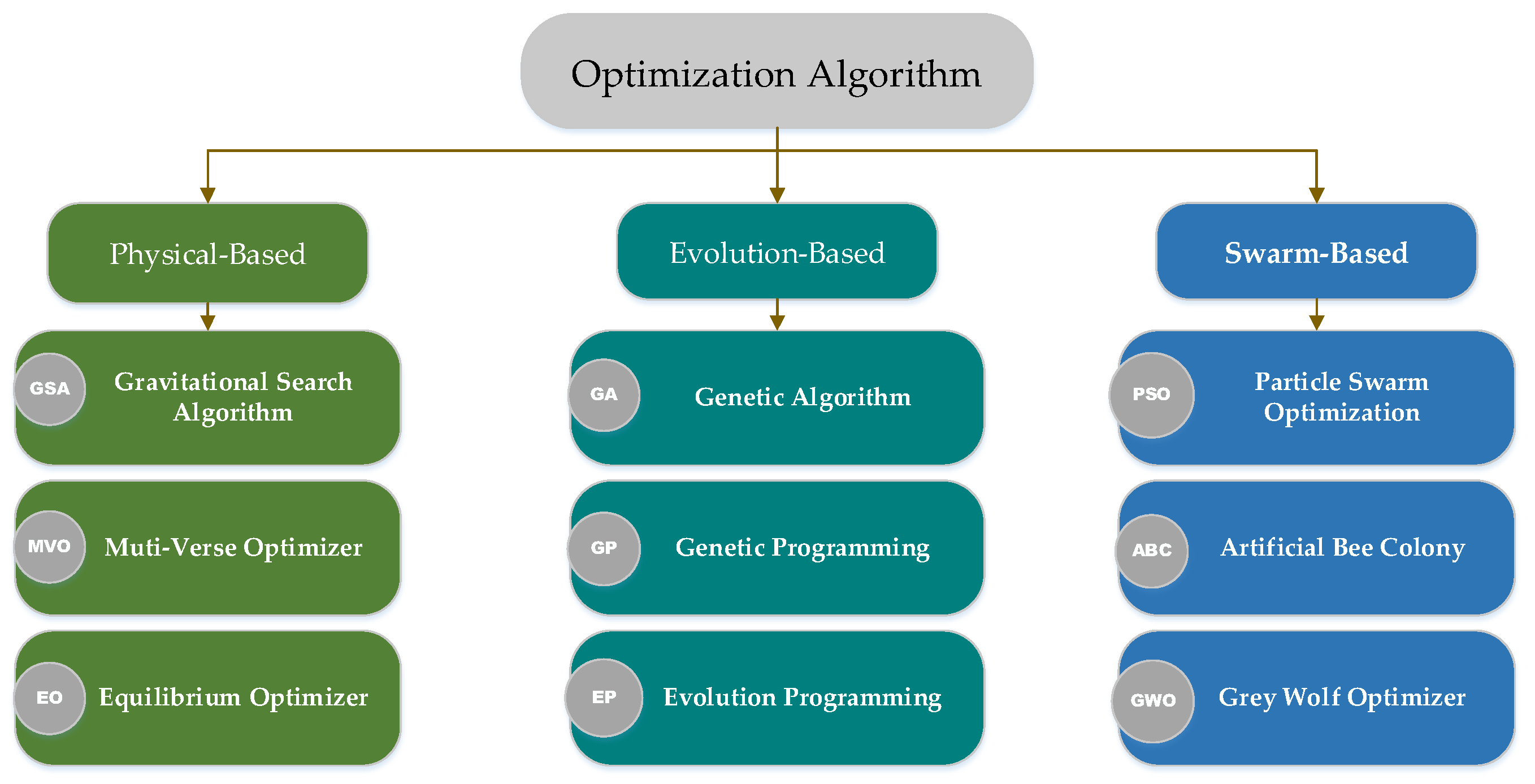
Optimization is a vibrant field with diverse applications in optimal control, disease treatment and engineering design [1,2,3,4,5]. In the past few years, modeling and implementing Metaheuristic Algorithms (MAs) have proved their worth [6,7,8,9]. Compared with other conventional optimization algorithms, MAs are widely used in engineering applications for the following reasons: first and foremost, the concepts of MAs are accessible and easy to implement; second, MAs are better than local search algorithms; and finally, they do not need derivative-function information. Nature-inspired Metaheuristic Algorithms deal with optimization problems by mimicking biological or physical phenomena. MAs can be generally divided into three categories: the physical-based, the evolution-based and the swarm-based [10] algorithms, as shown in Figure 1. Although these MAs have some differences, they all benefit from the above advantages.
A variety of MAs are introduced in this paper. To be specific, the physical-based algorithm originates from the physical, chemical phenomenon and the human intelligence. In the literature [11], the Gravitational Search Algorithm (GSA), which works on gravity and mass interactions, is discussed. The search agent is a set of interacting masses based on the Newtonian gravitation. Furthermore, GSA is wildly used in the field of machine learning. Other typical representatives are the Muti-Verse Optimizer (MVO) [12], Simulated Annealing algorithm (SA) [13], Equilibrium Optimizer (EO) [14], etc. In the following, one of the types which is affected by the biological evolution is introduced. In 1992, the genetic algorithm (GA) [15] was the first and the most popular algorithm to solve optimization problems, and it was established by Holland. The GA is derived from the laws of Darwinian evolution. This algorithm is regarded as one of the most effective algorithms, and it has been commonly utilized to solve substantial optimization problems with two recombination and mutation operators. This algorithm has been proposed with various modified and recombination versions [16]. Differential Evolution (DE) [17], Evolutionary Deduction (ED) [18] and Genetic Programming (GP) [19] are some well-known algorithms in this category. It is well-known that the swarm-based algorithm is a common approach, which derives from the survival habits of animal groups. Particle Swarm Optimization (PSO) [20] is an outstanding instance of the swarm-based algorithm, which was inspired by the swarm behavior of natural animals, such as birds and fish, in 1995. Since then, PSO has attracted humans’ core attention and formed a desirable research subject called swarm intelligence. Another typical algorithm was the Artificial Bee Colony (ABC) [21], which was proposed by Karaboga in 2005; it originated from the collective behavior of bees. Like other Metaheuristic Algorithms, this algorithm also has some shortcomings. Therefore, a modified version was introduced later. Yang introduced a novel algorithm based on the luminosity of fireflies in 2010 [22]. The brightness or light of each firefly is compared to that of other fireflies. Of course, fireflies sometimes fly randomly, which improves the modified version of this algorithm. In addition, another swarm-based algorithm called Bat Algorithm (BA) [23] was proposed by Yang et al. in 2010; it was derived from the echolocation of bats. The Grey Wolf Optimizer (GWO) [6] is a well-established swarm intelligence algorithm that was developed by Mirjalili et al. in 2016. Moreover, the GWO was inspired by the social life and hunting activities of wolves. In 2019, Heidari et al. proposed the Harris Hawks Optimization (HHO) [24], which simulated the unique cooperative hunting of Harris hawks. Inspired by the biological behaviors of prey and predators, Faramarzi et al. established the swarm-based Marine Predators Algorithm (MPA) in 2020 [25].
In 2018, Lin et al. proposed a hybrid optimization method of the Beetle-Antenna Search Algorithm and Particle Swarm Optimization (PSO) [26]. The BAS has good optimizing speed and accuracy in low-dimensional optimization problems, but it is easy to fall into local optimization in high-dimensional problems. Combining the PSO algorithm with the BAS can improve the BAS’s optimization ability. Moreover, the BAS [27] can be applied to other Metaheuristic Algorithms to overcome the shortcomings of a single algorithm. For instance, Zhou et al. proposed a Flower-Pollination Algorithm (FPA) based on the Beetle-Antennae Search Algorithm to overcome the slow convergence problem of the original FPA algorithm [28]. The experimental results show that the improved optimization algorithm has a faster convergence rate. An improved Artificial-Bee-Colony Algorithm (ABC) [29] based on the Beetle-Antenna Search (BAS–ABC) was proposed by Cheng et al. in 2019 [30]. This algorithm makes use of the position-update ability of BAS to avoid the randomness of searching, so that the original algorithm can converge to the optimal solution more quickly. The Beetle-Antennae Search Based on Quadratic Interpolation (QIBAS) is an effective swarm intelligence optimization algorithm. QIBAS has been applied to the Inverse Kinematics Solution Algorithm of Electric Climbing Robot Based on the Improved Beetle-Antennae Search [31]. It is universally believed that this improved algorithm improves the convergence accuracy. The teaching–Learning-Based Optimization (TLBO) [32] is a very mature swarm intelligence optimization algorithm, which has been used in the improvement and hybrid of many MAs. Tuo et al. proposed a hybrid algorithm based on Harmonious Search (HS) and Teaching–Learning-Based Optimization for complex high-dimensional problems [33]. HS has a strong global search capability, but its convergence speed is slow. TLBO can make up for this deficiency to increase the convergence rate. Keesari et al. used the TLBO algorithm to solve the job-shop-scheduling problem [34] and compared with other optimization algorithms. The experimental results show that TLBO algorithm is more efficient in the job-shop-scheduling problem. In order to solve the problem that the TLBO algorithm is prone to local convergence in complex problems, Chen et al. designed the local learning and self-learning methods to improve the original TLBO algorithm [35]. It is proved that the improved TLBO has a better global search ability than other algorithms by testing on a few functions. Quasi-Reflection-Based Learning (QRBL) [36] is a variant of Opposition-Based Learning (OBL) [37], and it is an effective intelligent optimization technique. QRBL can be applied to Biogeography-Based Optimization (BBO) [38], Ion Motion Optimization (IMO) [39] and Symbiotic Organisms Search (SOS) [40]. The modified algorithm with QRBL has better convergence speed and the better ability to avoid the local optimal than the basic algorithm.
The Gorilla Troops Optimizer (GTO) [41] is a new swarm intelligence optimization algorithm that was established by Abdollahzadeh et al. in 2021. The inspiration of GTO is the migration, competition for adult females and following behavior of the gorilla colony. Currently, it has been applied to several subject-design and engineering-optimization problems. However, like other swarm intelligence optimization algorithms, GTO is difficult to obtain a balance between exploration and exploitation due to the randomness of the optimization process. Therefore, the algorithm still has some problems, such as low accuracy, slow convergence and ease of falling into local optimal. It is worth mentioning that the No Free Lunch (NFL) [42] theorem indicates that no algorithm can solve all optimization problems perfectly. Therefore, this theorem and the defects of GTO prompt us to improve and develop the modified swarm-based algorithm to deal with more engineering problems:
(1)
A modified GTO, which is called MGTO, is proposed in this paper. The modified algorithm introduces three improvement strategies. Firstly, the Quadratic Interpolated Beetle-Antennae Search (QIBAS) [31] is embedded into the GTO that can get the diversity of the silverback’s position. In addition, Teaching–Learning-Based Optimization (TLBO) [32] is hybridized with GTO to stabilize the performance between the silverback and other gorillas. Finally, the Quasi-Reflection-Based Learning (QRBL) [36] mechanism is used to enhance the quality of the optimal position.
(2)
To verify the effectiveness of the MGTO, 23 classical benchmark functions, 30 CEC2014 benchmark functions and 10 CEC2020 benchmark functions are adopted to conduct a simulation experiment. The performance of the MGTO is evaluated through a variety of comparisons with the basic GTO and eight state-of-the-art optimization algorithms.
(3)
Furthermore, the MGTO is applied to solve the welded-beam-design problem, pressure-vessel-design problem, reducer problem, compression/tension-spring problem, three-bar-truss-design problem, crash-worthiness-design problem and string-design problem. The experimental results indicate that MGTO has a strong convergence ability and global search ability.
The rest of this paper is organized as follows: Section 2 introduces the basic GTO. In Section 3, three strategies and the modified GTO named MGTO are proposed. The experimental results and the discussion of this work are presented in Section 4. In Section 5, the MGTO is tested to solve seven kinds of real-world engineering problems. Finally, the conclusion and future work are given in Section 6.

2. Gorilla Troops Optimizer (GTO)

The Gorilla Troops Optimizer is a swarm-inspired algorithm that simulates the social life of gorillas. The gorilla is a social animal, and it is the largest primate on earth at present. Because of the white hair on its back, the adult male is also known as a silverback.
A gorilla group always consists of an adult male gorilla, several adult female gorillas and their offspring. Among them, the adult male gorilla is the leader, whose responsibilities are to defend the territory, make decisions, direct other gorillas to find abundant food and so on. The research shows that the male and female gorillas deviate from their birth with high probability. Generally, the male gorillas incline to abandon their quondam groups for appealing female gorillas, and then they will form a new group. Nevertheless, the male gorillas sometimes prefer to stay in the group in which they were born, with the hope that they will have the chance to dominate the whole group one day. The fierce competition for females between male gorillas is inevitable. Male gorillas can expand their territory by competition. The relationship between male and female gorillas is close and stable, while the relationship among female gorillas is cold relatively.
This algorithm includes two stages: Exploration and exploitation. Five different operators emulate the optimization operation for the behavior of gorillas in this algorithm. There are three operators in the exploration stage: moving to an undiscovered position, moving toward the other gorillas, moving to a known position. In the exploitation stage, two different operators of tracking the silverback and competing for adult females are adopted to improve the search performance.

2.1. Exploration

The operation procedures of the exploration stage are described in this subsection. It is commonly known that a gorilla group is governed by a silverback who has the capacity to conduct all actions. Sometimes gorillas will go to other places which they have visited before or that are new to them in nature. At each optimization operation stage, the optimal candidate solution is regarded as a silverback solution. Furthermore, three mechanisms at this stage are introduced.
Equation (1) is used to denote three mechanisms in the exploration stage. In the equation, p is a parameter ranging from 0 to 1 which is utilized to choose the mechanism of migration for an unknown position. For the sake of clarity, the mechanism for migration to an unknown position will be chosen when rand < p. Then, if rand ≥ 0.5, the second mechanism, that of movement toward the other gorillas, will be selected. If rand < 0.5, the mechanism for migration to a known position will be selected.
G X t + 1 = U B L B × r 1 + L B r a n d < p r 2 C × X r t + L × H r a n d 0.5 X i L × L × X t G X r t + r 3 × X t G X r t r a n d < 0.5
where GX(t+1) indicates the candidate position vector of the gorilla at the next iteration, and X(t) is the current position vector of the gorilla. Moreover, r1, r2, r3 and rand are the random values between 0 and 1. UB and LB indicate the upper and lower bounds of the variables, respectively. Xr and GXr are the candidate position vectors of gorillas that are selected randomly.
The equations that are used to calculate C, L and H are as follows:
C = F × 1 I t M a x I t
where It indicates the current iteration value, and MaxIt is the maximum iteration value. At the initial stage, the variation values are generated in a large interval, and then the changed interval of variation values will decrease in the final optimization stage. F can be calculated by the following equation:
F = cos 2 × r 4 + 1
where r4 is a random value that is in between [−1,1].
L is a parameter for which the calculation equation is as follows:
L = C × l
where l is a random value from 0 to 1. Moreover, the Equation (4) is utilized to simulate the silverback leadership. Because of inexperience, silverback gorillas always hard to make the correct decisions to find food or manage the group. However, they can obtain adequate experience and extreme stability in the leadership process. Additionally, H in Equation (1) is calculated by Equation (5). Z in Equation (5) is calculated by Equation (6), where Z is a random value in the range of [−C, C]:
H = Z × X t
Z = C , C
At the end of the exploration, a group operation is performed to calculate the cost of all GX solutions. If the cost is identified as GX(t) < X(t), the X(t) solution will be substituted by GX(t) solution. Therefore, the best solution at this stage is regarded as the silverback, as well.

2.2. Exploitation

In the exploitation stage of the GTO algorithm, the two behaviors of following the silverback and competing for adult females are adopted. The silverback leads all the gorillas in the group, and it is responsible for various activities in the group. Competing for adult females is another behavior. The C value indicates that the adult males can choose to follow the silverback or compete with other males. W is a parameter which should be set before the optimization operation. If C satisfies different conditions, the above mechanism will be selected.

2.2.1. Following the Silverback

When the silverback and other gorillas are young, they can perform their duties well. For instance, male gorillas follow the silverback easily. Moreover, each member can influence other members. That is to say, if CW, the strategy will be performed. By mimicking this behavior, Equation (7) is used to illustrate this mechanism, as follows:
G X t + 1 = L × M × X t X s i l v e r b a c k + X t
where Xsilverback is the vector of the silverback, which presents the optimal solution. M can be expressed as follows:
M = 1 N i = 1 N G X i t g 1 g
where GXi(t) refers to the vector position of each candidate gorilla at iteration, t; N indicates the sum of gorillas; and g is estimated by Equation (9) as follows:
g = 2 L

2.2.2. Competition for Adult Females

Competing for females with other male gorillas is a main stage of puberty for young gorillas. This competition is always fierce, which will persist for days and affect other members. Equation (10) is used to emulate this behavior:
G X i = X s i l v e r b a c k X s i l v e r b a c k × Q X t × Q × A
Q = 2 × r 5 1
A = β × E
E = N 1 , r a n d 0.5 N 2 , r a n d < 0.5
where Q is adopted to simulate the impact, which is calculated by Equation (11). Moreover, r5 is a random value between 0 and 1. Equation (12) is used to calculate the coefficient vector of the violence degree in conflict, where β is the parameter that needs to be given before the optimization operation. E is used to simulate the effect of violence on the solution’s dimensions. If rand ≥ 0.5, E will be equal to a random value in the normal distribution and the problem’s dimensions. However, if rand < 0.5, E will be equal to a random value in the normal distribution; rand is a random value between 0 and 1.

3. Modified Algorithm Implementation

3.1. Beetle-Antennae Search Based on Quadratic Interpolation (QIBAS)

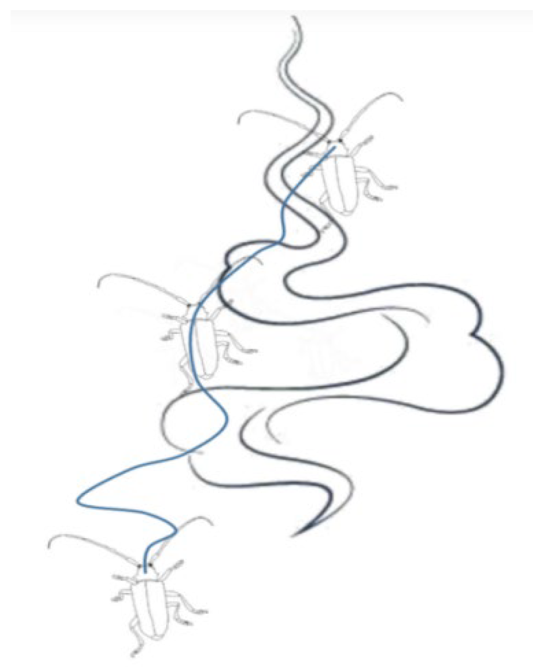
The beetle hunts through two antennae. Inspired by this, the Beetle-Antennae Search (BAS) algorithm was proposed by Jiang et al. in 2017 [27]. Different odors in the space correspond to different function values. The beetle can detect odor values on both sides of itself and search for the position with the highest odor. The position with the highest odor is the specific position of food. The habits of the beetle are shown in Figure 2, where the black line represents the propagation of odor, and the blue line denotes the trajectory of the beetle.

3.1.1. Searching Behavior of Beetles

To model the searching behavior, the random direction of the beetle’s searching is represented as follows:
b = r a n d s k , 1 r a n d s k , 1
where b is the unit vector, rands is a random value and k is the dimension of the position.
In addition, the searching behavior of the left and right sides of the beetle are given, respectively, as follows:
x l = x t + d × b x r = x t d × b
where xr indicates the right side of searching area, xl denotes the left side of searching area and d represents the length of the antennae.

3.1.2. Detecting Behavior of Beetles

To simulate the detecting behavior, the iterative model corresponding to the odor detection is as shown below:
x t + 1 = x t s × b × s i g n f x l f x r
where x represents the position of the beetle, and f(x) represents the strength of the odor at position x . The maximum value of f(x) donates the source point of the odor, and s is the step length of the searching. The function, sign(x); the antennae length, d; and the step length, s, are represented as follows:
s i g n x = 1 i f x > 0 0 i f x = 0 1 o t h e r w i s e
d t + 1 = 0.95 d t + 0.01
s t + 1 = 0.95 s t

3.1.3. Quadratic Interpolation Based on Beetle-Antennae Search (QIBAS)

The BAS algorithm has the advantages of accessible principle and high convergence speed. In order to further improve its ability to solve optimization problems, the quadratic interpolation operator is introduced, which can be presented as follows:
x i = 1 2 x l k 2 x b k 2 f x r + x b k 2 x r k 2 f x l + x r k 2 x l k 2 f x b x l k x b k f x r + x b k x r k f x l + x r k x l k f x b
where k is the dimension of the position, and xb denotes the global optimal solution.
The quadratic interpolation is adopted to obtain a new solution, xi, which varies from the existing solution, xt. The fitness values of the two positions are compared to determine whether xt is preserved or replaced.

3.2. Teaching–Learning-Based Optimization

The Teaching–Learning-Based Optimization (TLBO) was proposed in 2012; it was inspired by the influence of the teacher on the output of learners [32]. The output is evaluated by results and grades. Generally, a teacher is considered to be a knowledgeable person who trains and shares knowledge with students. Learners earn better grades with the help of a well-qualified teacher. Moreover, learners can learn interactively, as well, to improve their own knowledge. The result of learners can be considered as the “fitness”, and the teacher can be considered as the optimal solution currently.

3.2.1. Teacher Phase

As mentioned above, a knowledgeable teacher can increase the mean level of a class. However, it is difficult for the teacher to bring learners up to the same level as him/her. In fact, a teacher can only improve the mean of the class to a certain degree according to the capability of this class. It is a random process that relies on some factors. Mi represents the mean at iteration, i. Ti is the teacher who strives to bring Mi up to his/her level. Hence, the new mean can be designated as Mnew. The updated solution based on the difference between the current mean and new mean is given as follows:
D i f f e r e n c e _ M e a n i = r i M n e w T F M i
where TF is the teaching factor to change the mean, and ri is a random value ranging from 0 to 1. The value of TF can be represented as follows:
T F = r o u n d 1 + r a n d 0 , 1
To reduce the difference, the existing solution is modified according to the following equation:
X n e w , i = X o l d , i + D i f f e r e n c e _ M e a n i

3.2.2. Learner Phase

Learners increase their knowledge in two different patterns: one is the input of the teacher, and the other is the interaction among themselves. Learners interact randomly with other learners through group cooperation, presentations, debates, etc. Learners learn from others who have more knowledge. The modified learner can be expressed as follows:
X n e w , i = X o l d , i + r i X i X j ; i f   f X j < f X i
X n e w , i = X o l d , i + r i X j X i ; i f   f X i < f X j

3.3. Quasi-Reflection-Based Learning

A new Quasi-Reflection-Based Learning (QRBL) mechanism was established based on Opposition-Based Learning (OBL) and Quasi-Opposition-Based Learning (QOBL) by Ewees et al. in 2018. The quasi-reflection number, xqr, of the solution, x, is obtained as follows:
x q r = r a n d l b + u b 2 ,   x
where rand((lb+ub/2),x) is a random number which distributes uniformly between (lb+ub/2) and x. The quasi-reflection value can be extended into D-dimensional space, which is expressed as follows:
x i q r = r a n d l b i + u b i 2 ,   x i

3.4. The Proposed MGTO

Like other swarm intelligence algorithms, GTO still falls into local optimum and suffers from slow convergence easily. To overcome these shortcomings and further enhance the performance of the GTO, a modified MGTO is proposed that introduces QIBAS, TLBO and QRBL into the GTO. First, the QIBAS algorithm is employed to enrich the initial position of the silverback. Then TLBO is hybridized with the stage involving following the silverback into the exploitation phase. In this stage, the silverback can be considered as a teacher, and other gorillas learn from the silverback. Through this operation, the search ability of gorillas is enhanced, and the differences between the silverback and gorillas are reduced. Thirdly, QRBL is adopted to update the position of the silverback at the end of the stage, thus facilitating the quality of the optimal position.
In the initialization phase, the MGTO generates the random population, Xi, and initializes the position of the silverback. Then the QIBAS algorithm is used to calculate the search positions on both sides of the silverback. The NewPosition can be calculated by Equation (28). The quadratic interpolation function is employed to generate NewPosition1. NewPosition1 can be expressed by Equation (29). To choose an optimal position, the fitness values of these two positions are compared, and then, if the fitness value of the “new position” is better than the previous one, it will replace the previous position:
N e w p o s i t i o n = x t s × b × s i g n f x l f x r
N e w p o s i t i o n 1 = 1 2 x l k 2 S i l v e r b a c k 2 f x r + S i l v e r b a c k 2 x r k 2 f x l + x r k 2 x l k 2 f S i l v e r b a c k x l k S i l v e r b a c k f x r + S i l v e r b a c k x r k f x l + x r k x l k f S i l v e r b a c k
In the exploitation phase, the TLBO algorithm is adopted to update the behavior of following the silverback with 50% probability. The first step is calculating the mean, M, of the population. Secondly, the teach factor, F, and the difference, Difference, between gorillas and the silverback are calculated. In addition, the third step is to update the position, as shown below:
G X i = X o l d , i + D i f f e r e n c e _ M e a n i
In the final phase, in order to get a new position of the silverback, QRBL is used to generate the quasi-reflection position XSilverbackqr. By comparing the fitness values of XSilverback and XSilverbackqr, the position is selected from two positions as the final optimal position:
P o s i t i o n s _ R O L = r a n d l b i + u b i 2 ,   x i
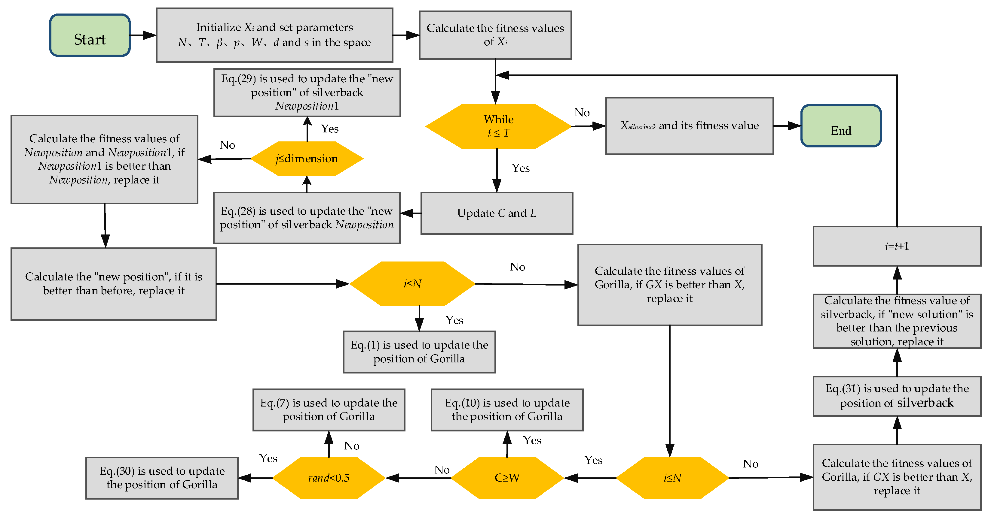
Eventually, repeating the steps mentioned until the maximum value of iterations is reached. The pseudo-code is represented below. And the flowchart of MGTO is shown in Figure 3.
Algorithm 1. The pseudo-code of MGTO
% MGTO setting
Inputs: the size of population, N; the maximum number of iterations, T; and parameters β, p, W, d and s.
Outputs: Xsilverback and its fitness value
% Initialization
Initialize the random population Xi (I = 1,2,…,N)
Calculate the fitness values of Xi
% Main Loop
while (stopping condition is not met) do
 Equation (2) is used to update C
 Equation (4) is used to update L
 Equation (28) is used to update the “new position” of silverback Newposition
for (j ≤ variables_no) do
  Equation (29) is used to update the “new position” of silverback Newposition1
end for
 Calculate the fitness values of Newposition and Newposition1
 if Newposition1 is better than Newposition, replace it
 if “new position” is better than the previous position, replace it
 % Exploration phase
for (each Gorilla (Xi)) do
  Equation (1) is used to update the position of Gorilla
end for
 % Establish group
 Calculate the fitness values of Gorilla
 if GX is better than X, replace it
 % Exploitation phase
for (each Gorilla (Xi)) do
  if (|C| ≥ 1) then
   if rand>0.5 then
    Update the position of Gorilla by using Equation (30)
   else
    Update the position of Gorilla by using Equation (7)
   end if
  else
  Update the position of Gorilla by using Equation (10)
  end if
end for
 % Establish group
 Calculate the fitness values of Gorilla
 if GX is better than X, replace it
 Equation (31) is used to update the position of silverback
 Calculate the fitness value of silverback
 if “new solution” is better than the previous solution, replace it
end while
Return Xsilverback and its fitness value

4. The Results and Discussion of Experiment

In this section, 23 classical benchmark functions are used to evaluate the performance of the proposed algorithm. Furthermore, nine optimization algorithms are selected for comparison, namely the Gorilla Troops Optimization (GTO) [41], Arithmetic Optimization Algorithm (AOA) [43], Salp Swarm Algorithm (SSA) [2], Whale Optimization Algorithm (WOA) [44], Grey Wolf Optimizer (GWO) [6], Particle Swarm Optimization (PSO) [20], Random-Opposition-Based Learning Grey Wolf Optimizer (ROLGWO) [45], Dynamic Sine–Cosine Algorithm (DSCA) [46] and Hybridizing Sine–Cosine Algorithm with Harmony Search (HSCAHS) [47]. For the sake of fairness, the maximum iteration and population size of all algorithms are set to 500 and 30, respectively.
The 23 classical benchmark functions can be divided into three categories: unimodal functions (UM), multimodal functions (MM) and composite functions (CM). The unimodal functions (F1~F7) have only one optimal solution that is fluently used to evaluate the exploration ability of the algorithm. The multimodal functions (F8~F13) are characterized by multiple optimal solutions. These functions can be utilized to evaluate the ability of jumping out from the local optimal solution in complex situations. The composite functions (F14~F23) are usually adopted to evaluate the stability of algorithms [48].
In addition, the benchmark functions (F1~F30) provided in CEC2014 and the benchmark functions (F1~F10) provided in CEC2020 are used in the other experiments [49]. These benchmarks are applied in many papers to evaluate the performance for the ability of solving problems. The standard to evaluate the performance of the optimization algorithm is whether it can keep the balance between exploration and development and avoid the local optimum.

4.1. The Experiments on Classical Benchmark

4.1.1. The Convergence Analysis

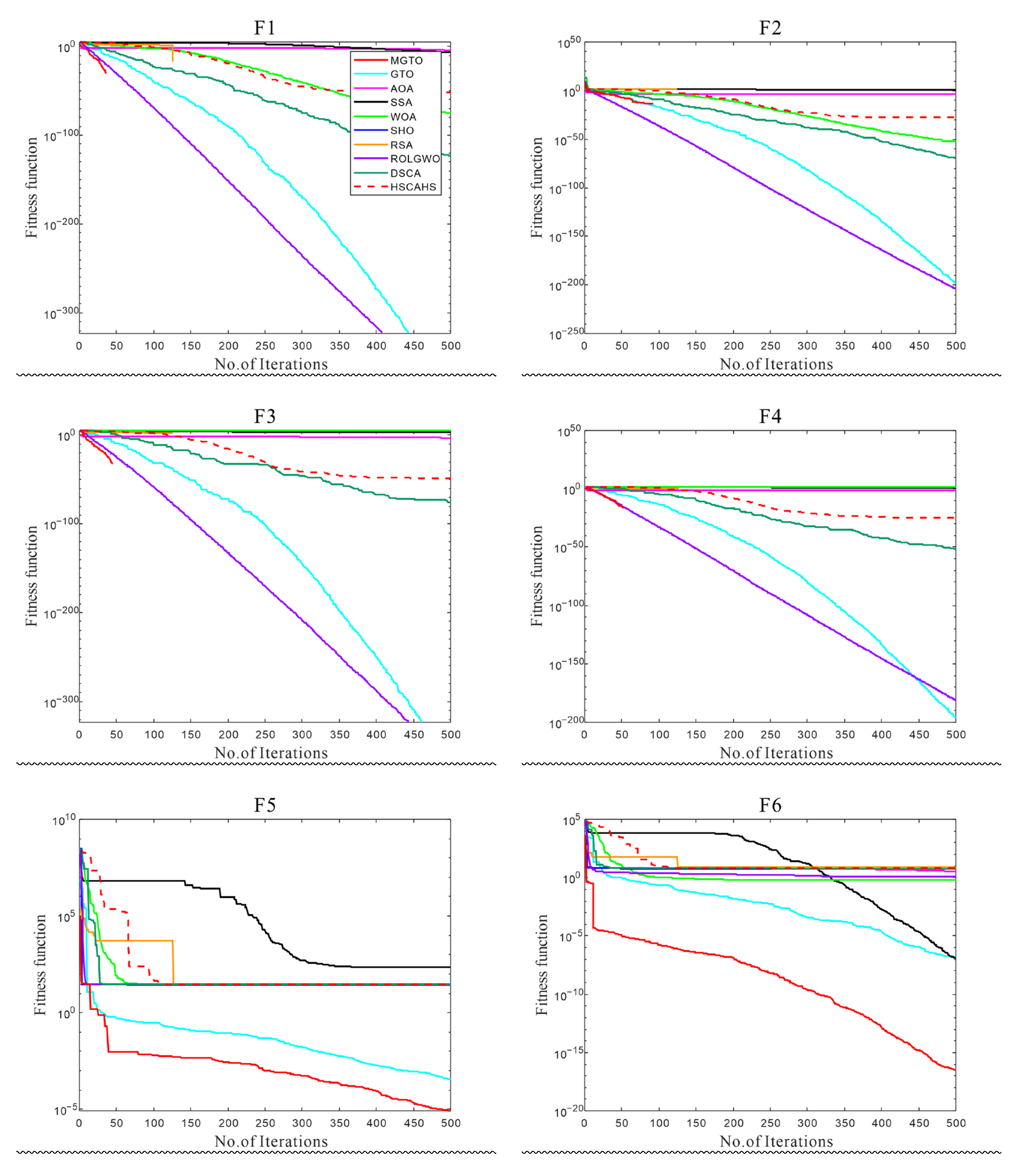
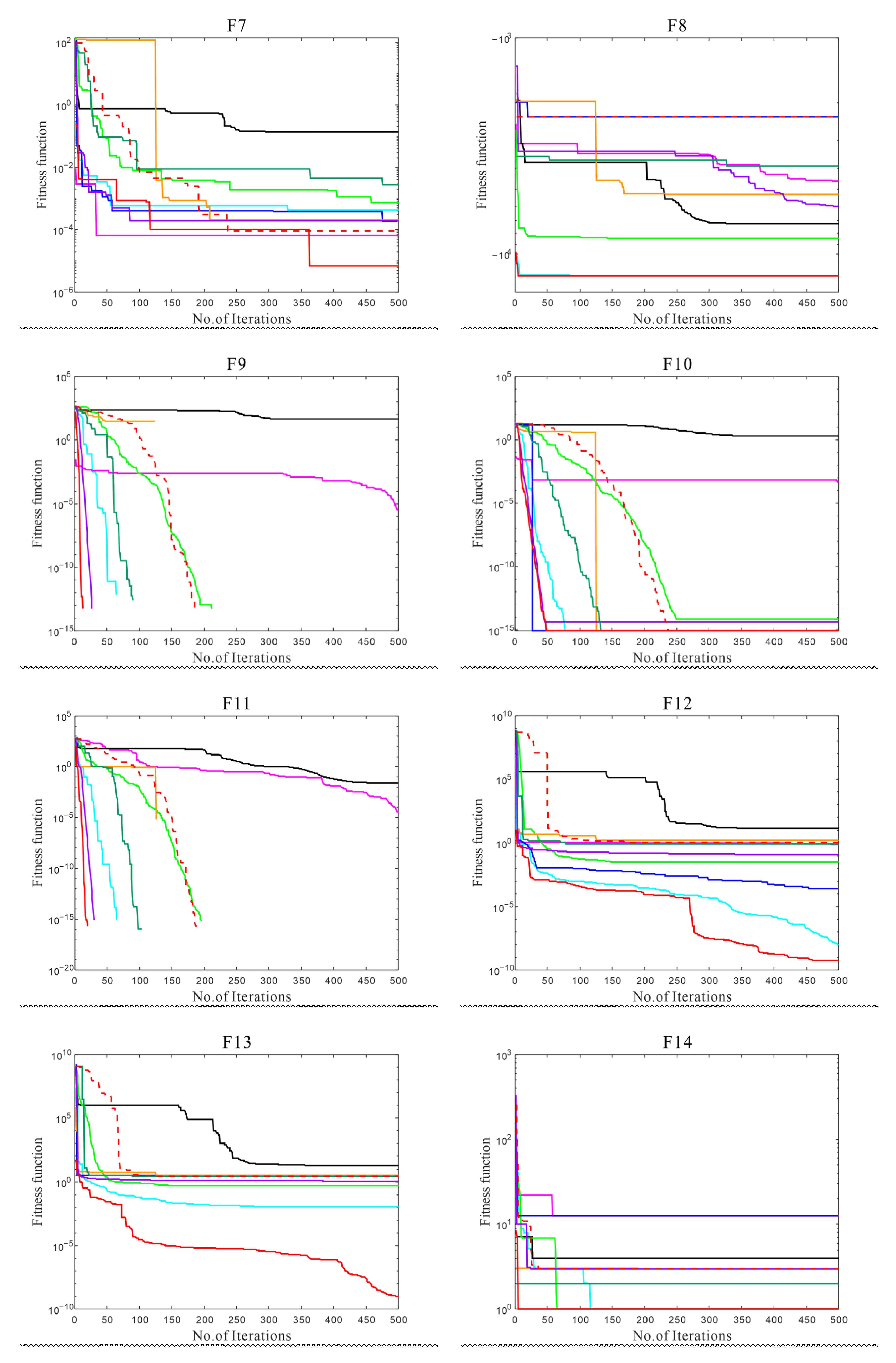
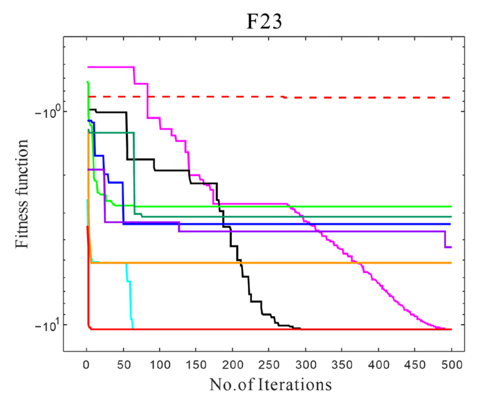
In order to evaluate the advantages of the MGTO algorithm on the benchmark functions, the MGTO is compared with traditional GTO, AOA, SSA, WOA, GWO, PSO, ROLGWO, DSCA and HSCAHS algorithms. The results in Figure 4 show that the proposed MGTO can achieve more efficient and better results compared with other optimization algorithms. Furthermore, this paper selects “semi-logarithms” to draw the convergence curve with the purpose of making the difference of curve convergence obviously. Because “0” has no logarithms, the iterative curve is interrupted in the figure. As shown in F1~F4, F9 and F11, the modified algorithm does not display curves in the subsequent process, just because it converges to 0, which reflects the high convergence accuracy of this algorithm. In addition, the proposed algorithm is superior to other algorithms in the benchmark-functions (F1~F13) experiments. It is obvious that the MGTO has the excellent property of keeping balance between exploration and exploitation when solving complicated problems. In the benchmark functions (F14~F23), the MGTO can obtain great superiority, thus indicating that the proposed algorithm is competitive in solving composite functions. However, the results of the benchmark functions (F17~F18) and the DSCA and PSO algorithms demonstrate that these algorithms give an excellent performance to obtain high-quality results. In summary, the MGTO performs well in benchmark functions (F14~F23). What is more, the MGTO can find excellent solutions compared with other algorithms in most cases. Thus, in the comparative experiment, the MGTO has certain advantages over the other algorithms. The effectiveness of the MGTO can be proved by the experiment results.

4.1.2. The Results of the Classical Benchmark

The results of 23 classical functions are listed in Table 1. All results are expressed by average value (Avg) and standard deviation (Std): The average value represents better convergence performance, and the standard deviation indicates the better stability. According to Table 1, it is obvious that the MGTO performs better in major tests. In particular, the optimal value of most functions is precisely calculated by MGTO, whereas other algorithms cannot find the optimal solution. Compared with the GTO, the proposed mechanism can improve the performance of obtaining the best solution.
Therefore, as far as numerous unimodal functions are concerned, the MGTO still remains the excellent searching performance, thus clearly proving the superiority of the exploitative ability in the MGTO. In contrast to unimodal functions, multimodal functions have multiple optimal solutions, which have many local optimal solutions. These multimodal functions are usually adopted to evaluate the convergence ability of algorithms. As Table 1 shows, the results can indicate that the proposed model has slight advantages in getting out of the local solutions. The primary cause is that the basic GTO has already provided competitive results. The functions F14~F23 can be used to test the stability and searching capability of algorithms. From Table 1, it can be seen that the performance of MGTO surpasses the traditional GTO, and the solution results of multiple functions are extremely close to the true value. Evidently, it can be concluded that the MGTO maintains high stability and exploitative ability consistently in the test.

4.2. The Experiments on CEC2014 and CEC2020

In this section, the CEC2014 tests are utilized to prove the performance of the MGTO. The results of the MGTO in complicated CEC2014 functions are compared with nine Metaheuristic Algorithms which are frequently quoted in the literature. The comparison results of CEC2014 benchmark functions are represented in Table 2. It can be seen from Table 2 that the MGTO provides the best results in 12 out of 30 cases for Avg and 15 out for 30 cases for Std. For other cases, it can be summarized as follows: SSA provides the best results in F24 and F25 for Avg; ROLGWO provides the best results in F6, F9 and F11 for Avg and F13 for Std; GTO provides the best results in F12 for Std; AOA provides the best results in F5 for Std; DSCA provides the best results in F6 for Std; and HSCAHS provides the best results in F9, F10, F11 and F16 for Std. In these cases, other algorithms are better than the MGTO, with a slightly different result. It can be proved that the MGTO has better efficiency and stability in solving global optimization problems. The MGTO can search the whole space consistently through subsequent iterations, and this can improve the convergence.
For CEC2020 benchmark functions, the functions (F1~F4) are as follows: translational rotation function, translational rotation schwefel function, translational rotation lunacek bi-rastrigin function and expansion rosenbrock’s plus griewangk function. F5~F7 functions are mixed functions. F8~F10 functions are composite functions. The results of CEC2020 calculated by MGTO, GTO, AOA, SSA, WOA, GWO, PSO, ROLGWO, DSCA and HACAHA are displayed in Table 3. According to Table 3, MGTO provides the best results in 6 out of 10 cases for Avg and 7 out for 10 cases for Std. For other cases, it can be summarized as follows: ROLGWO provides the best results in F3 for Avg, RSA provides the best results in F3 for Std and SSA provides the best results in F9 for Std. In function F4, all algorithms achieve the same Avg of 1.90E+03. Therefore, it can be concluded that the proposed algorithm can enhance the performance of GTO and solve CEC2020 functions better. Generally speaking, the MGTO has a better performance in solving optimization problems.

4.3. The Non-Parametric Statistic Test

Although the superiority of the MGTO was confirmed by the above benchmark functions, in order to further demonstrate the advantages of the MGTO, the Wilcoxon’s rank-sum test [50,51] with 5% accuracy is used to evaluate and research the difference between the proposed algorithm and other algorithms. The p-values of Wilcoxon’s rank-sum test are shown in Table 4, Table 5 and Table 6. The p-value less than 0.05 decides the significant differences between two algorithms. According to Table 4, Table 5 and Table 6, the superiority of the MGTO is statistically significant in most of the benchmark functions since most of the p-values are less than 0.05. Thus, the MGTO is considered to have significant advantages compared with other algorithms.

5. MGTO for Solving Engineering-Optimization Problems

In this section, seven engineering problems are used to evaluate the superiority of the MGTO, namely the welded-beam-design problem, pressure-vessel-design problem, speed-reducer-design problem, compression/tension-spring-design problem, three-bar-truss-design problem, car-crashworthiness-design problem and the tubular-column-design problem. The MGTO runs independently 30 times for each issue, with the maximum iterations setting at 500 and the population size at 30. In addition, the MGTO is compared to other algorithms in regard to dealing with engineering problems, as represented in the following tables; the corresponding conclusions are also discussed.

5.1. Welded-Beam Design

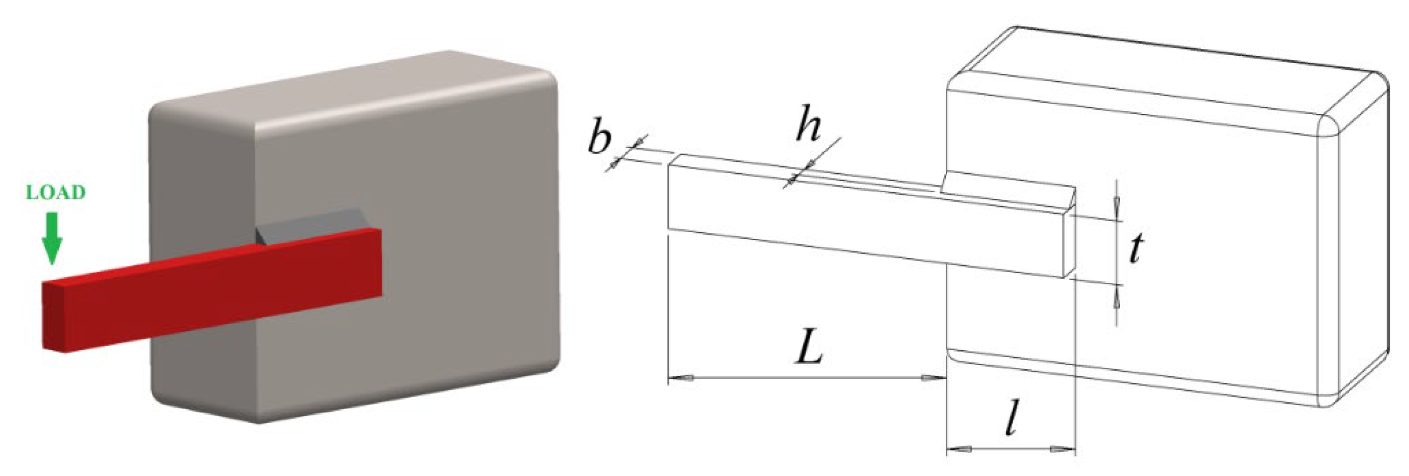
The welded-beam-design problem is a common engineering-optimization problem that was developed by Rao et al. [52]. Figure 5 offers a schematic diagram of a welded beam. In this problem, the constraints may be divided into four categories: shear stress, bending stress, buckling load and deflection of beam. The cost of welding materials is minimized as much as possible under the four constraints. Furthermore, there are four variables in the welded-beam-design problem: The thickness of the weld (h), the length of the weld (l), the height of the welded beam (t) and the thickness of the bar (b).
The mathematical model of the above problem is presented as follows:
Consider:
x = x 1 ,   x 2 ,   x 3 ,   x 4 = h ,   l ,   t ,   b
Minimize:
f ( x ) = 1.10471 x 1 2 x 2 + 0.04811 x 3 x 4 14.0 + x 2
Constraints:
g 1 ( x ) = τ ( x ) τ m a x g 2 ( x ) = σ ( x ) σ m a x g 3 ( x ) = δ ( x ) δ m a x g 4 ( x ) = x 1 x 4 0 g 5 ( x ) = P P C ( x ) 0 g 6 ( x ) = 0.125 x 1 0 g 7 ( x ) = 1.10471 x 1 2 + 0.04811 x 3 x 4 14.0 + x 2 5 0  
where we have the following:
τ ( x ) = ( τ ) 2 + 2 τ τ x 2 2 R + ( τ ) 2
τ = P 2 x 1 x 2 ,   τ = M R J ,   M = P L + x 2 2
R = x 2 2 4 + ( x 1 + x 3 2 ) 2
J = 2 2 x 1 x 2 x 2 2 4 + ( x 1 + x 3 2 ) 2
σ ( x ) = 6 P L x 3 2 x 4 ,   δ ( x ) = 6 P L 3 E x 3 3 x 4
P C ( x ) = 4.013 E x 3 2 x 4 6 36 L 2 1 x 3 2 L E 4 G
τ ( x ) = ( τ ) 2 + 2 τ τ x 2 2 R + ( τ ) 2
Variable range:
P = 6000   lb ,   L = 14   in ,   E = 30 × 10 6   psi ,   G = 12 × 10 6   psi
τ max = 13600   psi ,   σ max = 30000   psi ,   δ max = 0 . 25   in
The results of the MGTO and other comparative optimization algorithms are listed in Table 7. According to Table 7, it can be concluded that the MGTO was able to obtain the effective solution for welded-beam-design problems compared with other algorithms.

5.2. The Pressure-Vessel Problem

The pressure-vessel problem proposed by Kannan and Kramer [53] aims to reduce the cost of the pressure vessel under the pressure requirements. Figure 6 is a schematic diagram of the pressure vessel. The parameters include the following details: the thickness of the shell (Ts), the thickness of the head (Th), the inner radius of the vessel (R) and the length of the cylindrical shape (L).
Consider:
x = x 1   x 2   x 3   x 4 = T s   T h   R   L
Minimize:
f ( x ) = 0.6224 x 1 x 3 x 4 + 1.7781 x 2 x 3 2 + 3.1661 x 1 2 x 4 + 19.84 x 1 2 x 3
Constraints:
g 1 ( x ) = x 1 + 0.0193 x 3 0
g 2 ( x ) = x 3 + 0.00954 x 3 0
g 3 ( x ) = π x 3 2 x 4 4 3 π x 3 3 + 1296000 0
g 4 ( x ) = x 4 240 0
Variable range:
0 x 1 99 0 x 2 99 10 x 3 200 10 x 4 200
From Table 8, we can see that the optimal solution of the function obtained by the MGTO is 5734.9131, while x is equal to 0.7424, 0.3702, 40.3196 and 200. The lowest cost calculated by the MGTO is superior to other optimization algorithms, including the GTO [41], HHO [24], SMA [54], WOA [44], GWO [6], MVO [12] and GA [15], indicating that the proposed model has the merits in solving the pressure-vessel problem.

5.3. Speed-Reducer Design

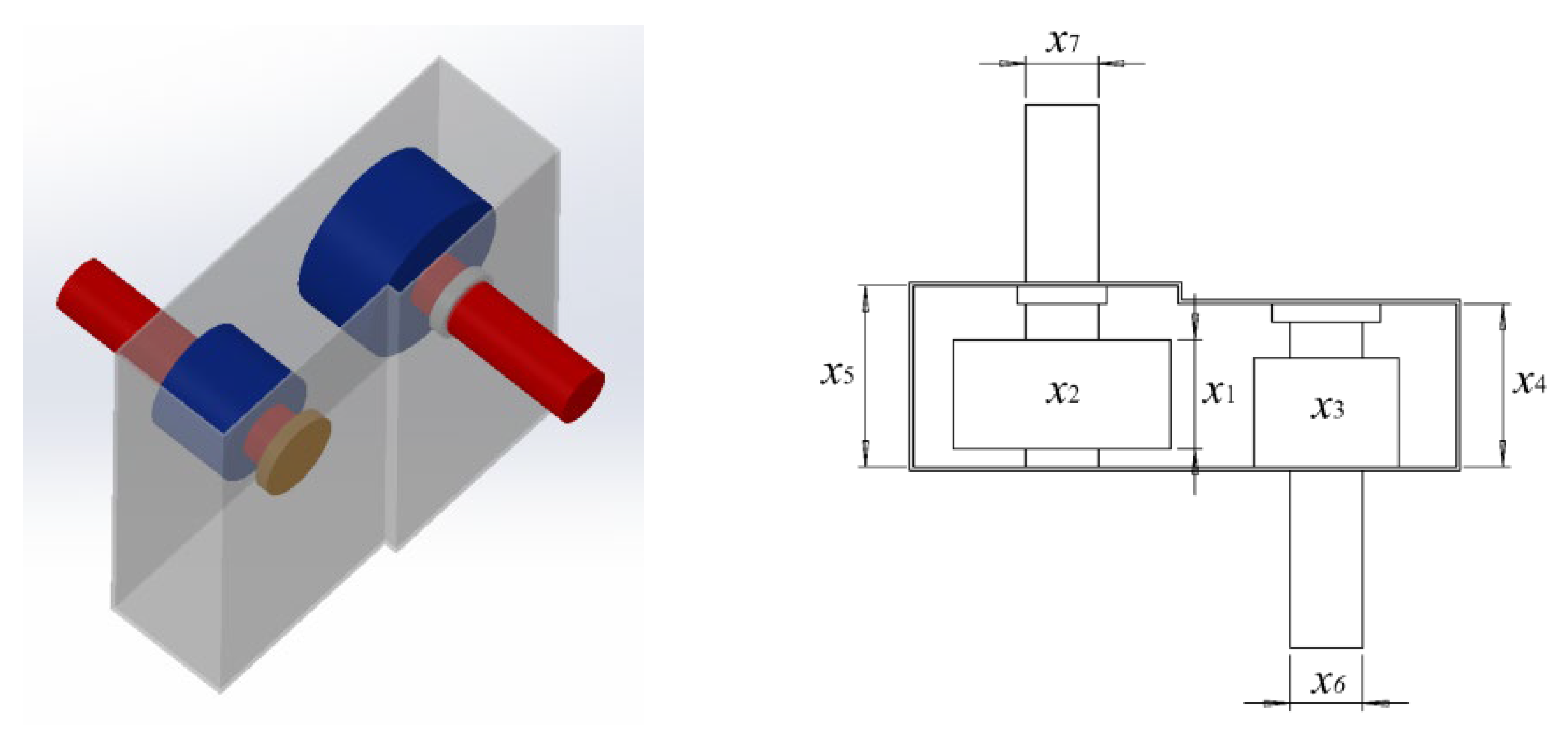
The main intention of this problem is to minimize the weights of the speed reducer, which can be limited by seven variables, namely the face width (x1), the teeth module (x2), the discrete design variables representing the teeth in the pinion (x3), the length of the first shaft between the bearings (x4), the length of the second shaft between the bearings (x5), the diameters of the first shaft (x6) and diameters of the second shaft (x7) [55]. In this case, there are four constraints that should be satisfied: covered stress, bending stress of the gear teeth, stresses in shafts and transverse deflection of the shafts, which are shown in Figure 7.
In addition, the formulas of this problem are expressed as follows:
Minimize:
f ( x ) = 0.7854 x 1 x 2 2   3.3333 x 3 2 + 14.9334 x 3 43.0934 1.508 x 1 x 6 2 + x 7 2 + 7.4777 x 6 3 + x 7 3
Constraints:
g 1 ( x ) = 27 x 1 x 2 2 x 3 1 0
g 2 ( x ) = 397.5 x 1 x 2 2 x 3 2 1 0
g 3 ( x ) = 1.93 x 4 3 x 2 x 3 x 6 4 1 0
g 4 ( x ) = 1.93 x 5 3 x 2 x 3 x 7 4 1 0
g 5 ( x ) = ( 745 x 4 x 2 x 3 ) 2 + 16.9 × 10 6 110.0 x 6 3 1 0
g 6 ( x ) = ( 745 x 4 x 2 x 3 ) 2 + 157.5 × 10 6 85.0 x 6 3 1 0
g 7 ( x ) = x 2 x 3 40 1 0
g 8 ( x ) = 5 x 2 x 1 1 0
g 9 ( x ) = x 1 12 x 2 1 0
g 10 ( x ) = 1.5 x 6 + 1.9 x 4 1 0
g 11 ( x ) = 1.1 x 7 + 1.9 x 5 1 0
Variable range:
2.6 x 1 3.6 0.7 x 2 0.8 17 x 3 28 7.3 x 4 8.3 7.8 x 5 8.3 2.9 x 6 3.9 5.0 x 7 5.5
The comparative optimization results of the speed-reducer-design problem are shown in Table 9.
Compared with the AO [56], PSO [20], AOA [43], MFO [57], GA [15], SCA [58] and MDA [59], it can be observed that the MGTO achieves 2995.4373, which is the best optimum weight. Thus, it can be certified that the MGTO has an obvious advantage in solving the speed-reducer-design problem.

5.4. Compression/Tension-Spring Design

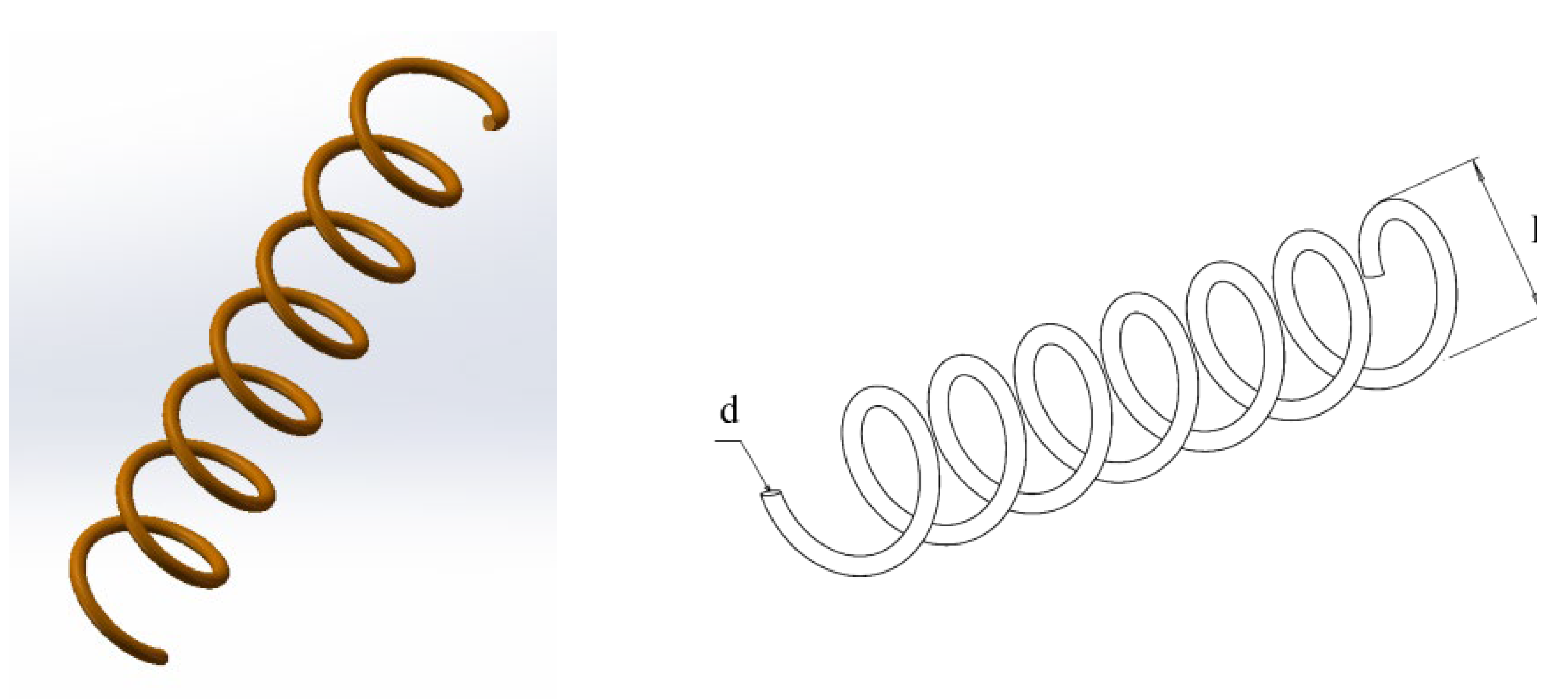
Compression/tension-spring-design problems minimize the weight of the spring (shown in Figure 8) [60]. The three constraints impacting frequency, shear stress and deflection should be satisfied in the optimization design. There are three variables displayed in Figure 8, namely the wire diameter (d), mean coil diameter (D) and the number of active coils (N).
The mathematical model is as follows:
Consider:
  x = [ x 1   x 2   x 3   x 4 = d   D   N ]
Minimize:
f ( x ) = x 3 + 2 x 2 x 1 2
Constraints:
g 1 ( x ) = 1 x 2 3 x 3 71785 x 1 4 0
g 2 ( x ) = 4 x 2 2 x 1 x 2 12566 x 2 x 1 3 x 1 4 + 1 5108 x 1 2 0
g 3 ( x ) = 1 140.45 x 1 x 2 2 x 3 0
g 4 ( x ) = x 1 + x 2 1.5 1 0
Variable range:
0.05 x 1 2.00 0.25 x 2 1.30 2.00 x 3 15.00
As Table 10 shows, the optimal solution calculated by MGTO is 0.0099, when variable x is equal to 0.05000, 0.3744 and 8.5465. According to the results, it is clear that the MGTO is capable of obtaining the best solution in comparison with other optimization algorithms.

5.5. Three-Bar-Truss Design

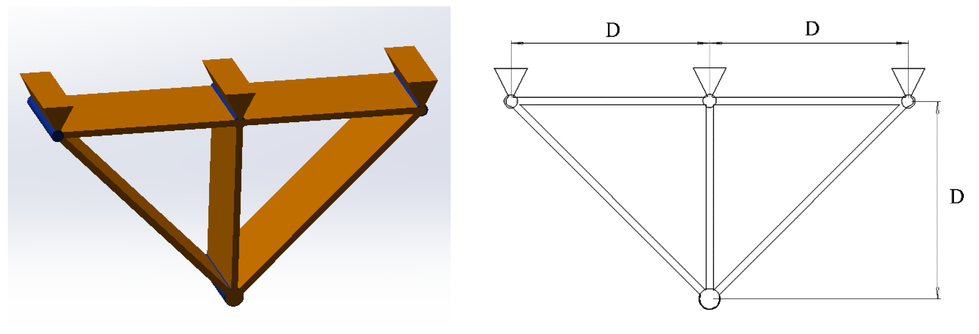
The three-bar-truss-design problem [61] is a typical engineering problem which can be utilized to evaluate the performance of algorithms. The main intention is to minimize the weight, which is subject to deflection, stress and buckling constraints on each of the truss members, by adjusting the cross-sectional areas A1, A2 and A3. It is illustrated in Figure 9.
The problem considers a non-linear function with three constraints and two decision variables. The mathematical model is given as follows:
Consider:
x = x 1   x 2 = A 1   A 2
Minimize:
f ( x ) = 2 2 x 1 + x 2 l
Constraints:
g 1 ( x ) = 2 x 1 + x 2 2 x 1 2 + 2 x 1 x 2 P σ 0
g 2 ( x ) = x 2 2 x 1 2 + 2 x 1 x 2 P σ 0
g 3 ( x ) = 1 2 x 2 + x 1 P σ 0
Variable range:
0 x 1 , x 2 1
where we have the following:
l = 100   cm ,   P = 2 K N / cm 2 ,   σ = 2 K N / cm 2
The results of the three-bar-truss-design problem are shown in Table 11, and it can be seen that the MGTO has significant superiority compared with other optimization algorithms in solving this problem. The proposed model can obtain the lowest optimum weight when x is equal to 0.7884 and 0.4081.

5.6. Car-Crashworthiness Design

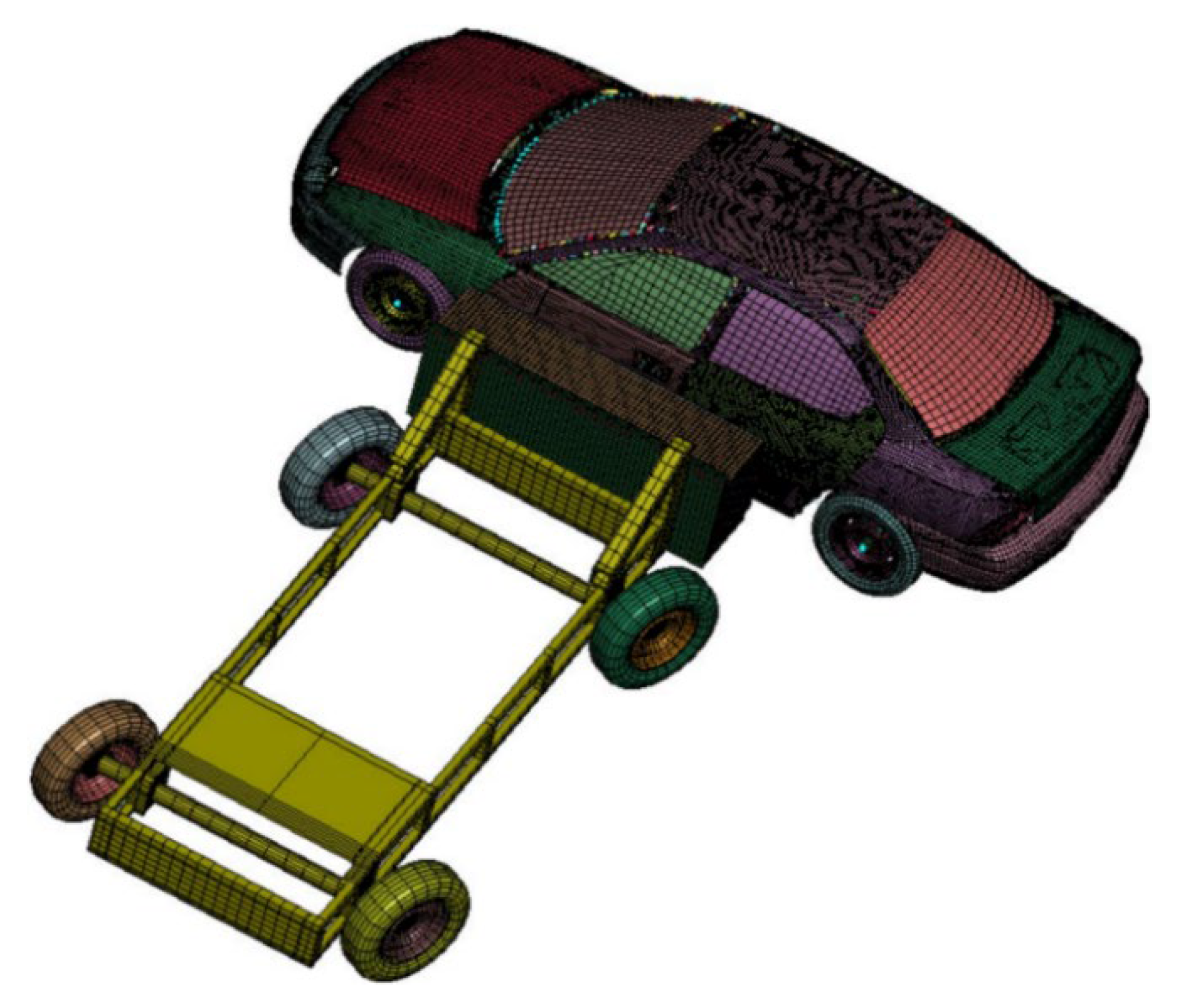
The car-crashworthiness-design problem proposed by Gu et al. aims to improve the safety of the vehicle and reduce casualties. The details are shown in Figure 10 [62].
In this case, eleven parameters are adopted to reduce the weight, namely the inside of the B-pillar, reinforcement of the B-pillar, the inside of the floor side, the crossbeam, the door beam, the door-strip-line reinforcement, the roof rail of the car (x1x7), the materials of inside of B-pillar and reinforcement of B-pillar (x8, x9), the thickness of barrier height and the impact position (x10, x11). The mathematical formula is represented as follows:
Minimize:
f ( x ) = 1.98 + 4.90 x 1 + 6.67 x 2 + 6.98 x 3 + 4.01 x 4 + 1.78 x 5 + 2.73 x 7
Constraints:
g 1 ( x ) = 1.16 0.3717 x 2 x 4 0.00931 x 2 x 10 0.484 x 3 x 9 + 0.01343 x 6 x 10 1
g 2 ( x ) = 0.261 0.0159 x 1 x 2 0.188 x 1 x 8 0.019 x 2 x 7 + 0.0144 x 3 x 5 + 0.0008757 x 5 x 10 + 0.080405 x 6 x 9 + 0.00139 x 8 x 11 + 0.00001575 x 10 x 11 0.32
g 3 ( x ) = 0.214 + 0.00817 x 5 0.131 x 1 x 8 0.0704 x 1 x 9 + 0.03099 x 2 x 6 0.018 x 2 x 7 + 0.0208 x 3 x 8 + 0.121 x 3 x 9 0.00364 x 5 x 6 + 0.0007715 x 5 x 10 0.0005354 x 6 x 10 + 0.00121 x 8 x 11 0.32
g 4 ( x ) = 0.074 0.061 x 2 0.163 x 3 x 8 + 0.001232 x 3 x 10 0.166 x 7 x 9 + 0.227 x 2 2 0.32
g 5 ( x ) = 28.98 + 3.818 x 3 4.2 x 1 x 2 + 0.0207 x 5 x 10 + 6.63 x 6 x 9 7.7 x 7 x 8 + 0.32 x 9 x 10 32
g 6 ( x ) = 33.86 + 2.95 x 3 + 0.1792 x 10 5.057 x 1 x 2 11.0 x 2 x 8 0.0215 x 5 x 10 9.98 x 7 x 8 + 22.0 x 8 x 9 32
g 7 ( x ) = 46.36 9.9 x 2 12.9 x 1 x 8 + 0.1107 x 3 x 10 32
g 8 ( x ) = 4.72 0.5 x 4 0.19 x 2 x 3 0.0122 x 4 x 10 + 0.009325 x 6 x 10 + 0.000191 x 11 2 4
g 9 ( x ) = 10.58 0.674 x 1 x 2 1.95 x 2 x 8 + 0.02054 x 3 x 10 0.0198 x 4 x 10 + 0.028 x 6 x 10 9.9
g 10 ( x ) = 16.45 0.489 x 3 x 7 0.843 x 5 x 6 + 0.0432 x 9 x 10 0.0556 x 9 x 11 0.000786 x 11 2 15.7
Variable range:
0.5 x 1 x 7 1.5 x 8 ,   x 9 0.192 ,   0.345 30 x 10 ,   x 11 30
The results of the car-crashworthiness-design problem are listed in Table 12. From the contents, we can see that the optimal weight obtained by the MGTO is 23.1894. Furthermore, it is certain that the MGTO is an efficient algorithm in solving the car-crashworthiness-design problem.

5.7. Tubular-Column Design

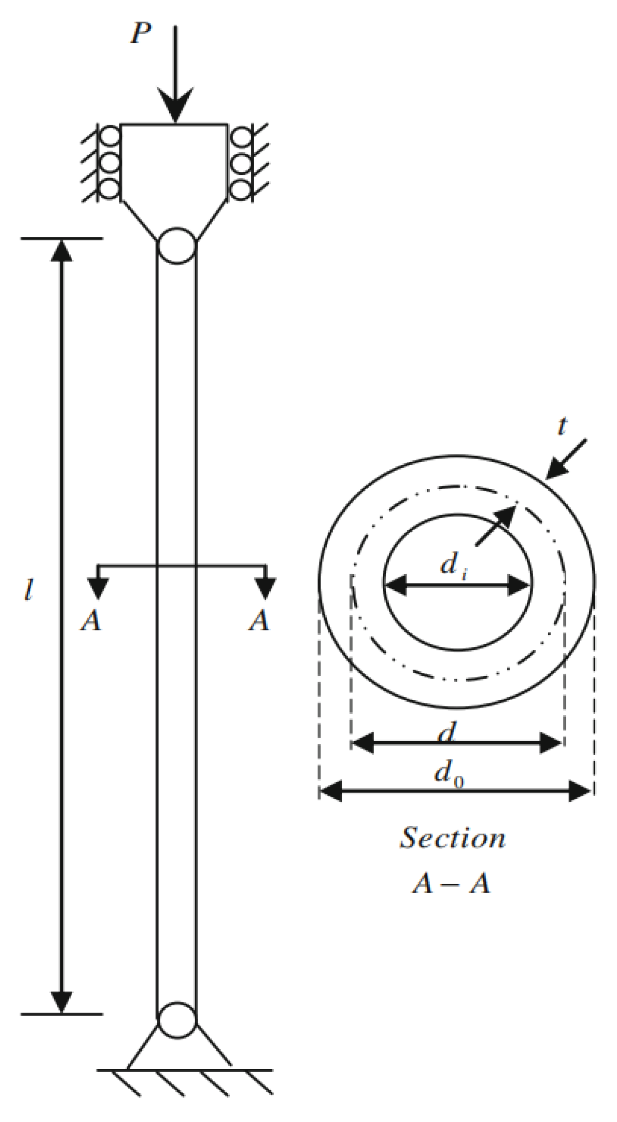
According to Figure 11, a tubular column is given to decrease the cost of supporting the compressive load, p = 2500 kgf, and it consists of the yield stress, elastic modulus and density.
The functions, including the material and manufacturing costs, are considered. The formulas can be expressed as follows:
Minimize:
f d ,   t = 9.8 d t + 2 d
Constraints:
g 1 = P π d t σ y 1 0
g 2 = 8 P L 2 π 3 E d t d 2 + t 2 1 0
g 3 = 2.0 d 1 0
g 4 = d 14 1 0
g 5 = 0.2 t 1 0
Variable range:
0.01 d ,   T 100
The comparative optimization results of the tubular-column-design problem are shown in Table 13.
The optimal solution obtained by the MGTO is 26.5313 when the variable x is 5.4511 and 0.2919. It is obvious that the proposed algorithm has advantages in solving the tubular-column-design problem.
In summary, the advantages of the proposed algorithm are shown in this section. Because the MGTO has great exploration and exploitation ability, it is superior to the traditional GTO and other existing algorithms in regard to performance. Therefore, the MGTO can be applied in practical engineering problems.

6. Conclusions and Future Work

The MGTO was proposed to modify the performance of GTO in this paper. Three strategies were used to modify the basic GTO. Firstly, the QIBAS algorithm was utilized to increase the diversity of the position of the silverback. Secondly, TLBO was introduced to the exploitation phase to reduce the difference of the silverback and gorillas. Thirdly, the QRBL generates the quasi-refraction position of the silverback to enhance the quality of the optimal position.
For the comprehensive evaluation, the proposed MGTO was compared to the basic GTO and eight other state-of-the-art optimization algorithms, namely AOA, SSA, WOA, GWO, PSO, ROLGWO, DSCA and HSCAHS, on 23 classical benchmark functions, 30 CEC2014 benchmark functions, and 10 CEC2020 benchmark functions. The statistical analysis results disclosed that MGTO is a very competitive algorithm and outperforms other algorithms in regard to exploitation, exploration, escaping local optimum, and convergence behavior. In order to further investigate the superior capability of the MGTO in solving real-word engineering problems, the proposed algorithm was compared with other algorithms, using seven constrained, complex and challenging problems. The obtained results confirmed the high competency of MGTO to optimize real-word problems with complicated and unknown search domains.
In future works, we hope that the MGTO will perform particularly well on more real-world problems, such as image segmentation, feature selection and so on. Moreover, the NFL theorem has also prompted researchers to improve more algorithms.
Author Contributions

Conceptualization, T.W. and D.W.; methodology, T.W. and D.W.; software, T.W. and H.J.; validation, T.W. and N.Z; formal analysis, T.W. and D.W.; investigation, T.W. and D.W; resources, D.W. and H.J.; data curation, T.W. and N.Z.; writing—original draft preparation, T.W. and D.W.; writing—review and editing, Q.L., K.H.A., L.A. and H.J.; visualization, T.W. and D.W.; supervision, D.W. and H.J.; funding acquisition, D.W., K.H.A. and H.J. All authors have read and agreed to the published version of the manuscript.

Funding

This work was funded by National Education Science Planning Key Topics of the Ministry of Education—“Research on the core quality of applied undergraduate teachers in the intelligent age”(DIA220374).

Institutional Review Board Statement

Not applicable.

Informed Consent Statement

Not applicable.

Data Availability Statement

Not applicable.

Acknowledgments

The authors would like to thank the Deanship of Scientific Research at Umm AI-Qura University for supporting this work thought grant (22UQU4320277DSR14). The authors would like to thank the anonymous reviewers and the editor for their careful reviews and constructive suggestions to help us improve the quality of this paper.

Conflicts of Interest

The authors declare that they have no conflict of interest.

References

  1. Khajehzadeh, M.; Iraji, A.; Majdi, A.; Keawsawasvong, S.; Nehdi, M.L. Adaptive Salp Swarm Algorithm for Optimization of Geotechnical Structures. Appl. Sci. 2022, 12, 6749. [Google Scholar] [CrossRef]
  2. Mirjalili, S.; Gandomi, A.H.; Mirjalili, S.Z.; Saremi, S.; Faris, H.; Mirjalili, S.M. Salp Swarm Algorithm: A Bio-Inspired Optimizer for Engineering Design Problems. Adv. Eng. Softw. 2017, 114, 163–191. [Google Scholar] [CrossRef]
  3. Das, S.; Das, P.; Das, P. Chemical and Biological Control of Parasite-Borne Disease Schistosomiasis: An Impulsive Optimal Control Approach. Nonlinear Dyn. 2021, 104, 603–628. [Google Scholar] [CrossRef]
  4. Das, P.; Upadhyay, R.K.; Misra, A.K.; Rihan, F.A.; Das, P.; Ghosh, D. Mathematical Model of COVID-19 with Comorbidity and Controlling Using Non-Pharmaceutical Interventions and Vaccination. Nonlinear Dyn. 2021, 106, 1213–1227. [Google Scholar] [CrossRef]
  5. Das, P.; Das, S.; Upadhyay, R.K.; Das, P. Optimal Treatment Strategies for Delayed Cancer-Immune System with Multiple Therapeutic Approach. Chaos Solitons Fractal. 2020, 136, 109806. [Google Scholar] [CrossRef]
  6. Mirjalili, S.; Mirjalili, S.M.; Lewis, A. Grey Wolf Optimizer. Adv. Eng. Softw. 2014, 69, 46–61. [Google Scholar] [CrossRef] [Green Version]
  7. Liu, Q.; Li, N.; Jia, H.; Qi, Q.; Abualigah, L. Modified Remora Optimization Algorithm for Global Optimization and Multilevel Thresholding Image Segmentation. Mathematics 2022, 10, 1014. [Google Scholar] [CrossRef]
  8. Das, P.; Upadhyay, R.K.; Das, P.; Ghosh, D. Exploring Dynamical Complexity in a Time-Delayed Tumor-Immune Model. Chaos 2020, 30, 123118. [Google Scholar] [CrossRef]
  9. Das, P.; Das, S.; Das, P.; Rihan, F.A.; Uzuntarla, M.; Ghosh, D. Optimal Control Strategy for Cancer Remission Using Combinatorial Therapy: A Mathematical Model-Based Approach. Chaos Solitons Fractals 2021, 145, 110789. [Google Scholar] [CrossRef]
  10. Wang, S.; Jia, H.; Laith, A.; Liu, Q.; Zheng, R. An Improved Hybrid Aquila Optimizer and Harris Hawks Algorithm for Solving Industrial Engineering Optimization Problems. Processes 2021, 9, 1551. [Google Scholar] [CrossRef]
  11. Rashedi, E.; Nezamabadi-Pour, H.; Saryazdi, S. GSA: A Gravitational Search Algorithm. Inf. Sci. 2009, 179, 2232–2248. [Google Scholar] [CrossRef]
  12. Mirjalili, S.; Mirjalili, S.M.; Hatamlou, A. Multi-Verse Optimizer: A Nature-Inspired Algorithm for Global Optimization. Neural Comput. Appl. 2016, 27, 495–513. [Google Scholar] [CrossRef]
  13. Kirkpatrick, S.; Gelatt, C.D.; Vecchi, M.P. Optimization by Simulated Annealing. Science 1983, 220, 671–680. [Google Scholar] [CrossRef] [PubMed]
  14. Faramarzi, A.; Heidarinejad, M.; Stephens, B.; Mirjalili, S. Equilibrium Optimizer: A Novel Optimization Algorithm. Knowl.-Based Syst. 2020, 191, 105190. [Google Scholar] [CrossRef]
  15. Holland, J.H. Genetic Algorithms. Sci. Am. 1992, 267, 66–73. [Google Scholar] [CrossRef]
  16. Hussain, S.F.; Iqbal, S. Genetic ACCGA: Co-Similarity Based Co-Clustering Using Genetic Algorithm. Appl. Soft Comput. 2018, 72, 30–42. [Google Scholar] [CrossRef]
  17. Storn, R.; Price, K. Differential Evolution–A Simple and Efficient Heuristic for Global Optimization Over Continuous Spaces. J. Glob. Optim. 1997, 11, 341–359. [Google Scholar] [CrossRef]
  18. Yao, X.; Liu, Y.; Lin, G. Evolutionary Programming Made Faster. IEEE Trans. Evol. Comput. 1999, 3, 82–102. [Google Scholar]
  19. Koza, J.R. Genetic Programming: On the Programming of Computers by Means of Natural Selection; MIT Press: Cambridge, MA, USA, 1922. [Google Scholar]
  20. Kennedy, J.; Eberhart, R. Particle swarm optimization. In Proceedings of the ICNN95—International Conference on Neural Networks, Perth, WA, Australia, 27 November 1995–1 December 1995; pp. 1942–1948. [Google Scholar]
  21. Kiran, M.S.; Gunduz, M. A Novel Artificial Bee Colony-based Algorithm for Solving the Numerical Optimization Problems. Int. J. Innov. Comput. I 2012, 8, 6107–6121. [Google Scholar]
  22. Yang, X.S. Firefly algorithm. In Nature-Inspired Metaheuristic Algorithms; Luniver Press: Bristol, UK, 2010; Volume 2, pp. 1–148. [Google Scholar]
  23. Yang, X.S.; Gandomi, A.H. Bat Algorithm: A Novel Approach for Global Engineering Optimization. Eng. Comput. 2012, 29, 464–483. [Google Scholar] [CrossRef] [Green Version]
  24. Heidari, A.A.; Mirjalili, S.; Faris, H.; Aljarah, I.; Mafarja, M.; Chen, H. Harris Hawks Optimization: Algorithm and Applications. Future Gener. Comput. Systems. 2019, 97, 849–872. [Google Scholar] [CrossRef]
  25. Faramarzi, A.; Heidarinejad, M.; Mirjalili, S.; Gandomi, A.H. Marine Predators Algorithm: A Nature-Inspired Metaheuristic. Expert Syst. Appl. 2020, 152, 11337. [Google Scholar] [CrossRef]
  26. Lin, M.; Li, Q. A Hybrid Optimization Method of Beetle Antennae Search Algorithm and Particle Swarm Optimization. DEStech Trans. Eng. Technol. Res. 2018, 1, 396–401. [Google Scholar] [CrossRef] [Green Version]
  27. Jiang, X.; Li, S. BAS: Beetle Antennae Search Algorithm for Optimization Problems. Int. J. Robot. Control 2017. [Google Scholar] [CrossRef]
  28. Zhou, J.; Qian, Q.; Fu, Y.; Feng, Y. Flower pollination algorithm based on beetle antennae search method. In Smart Innovation, Systems and Technologies; Springer: Berlin/Heidelberg, Germany, 2022; pp. 181–189. [Google Scholar]
  29. Karaboga, D.; Akay, B. A Comparative Study of Artificial Bee Colony Algorithm. Appl. Math. Comput. 2009, 214, 108–132. [Google Scholar] [CrossRef]
  30. Cheng, L.; Yu, M.; Yang, J.; Wang, Y. An improved artificial bee colony algorithm based on beetle antennae search. In Proceedings of the 2019 Chinese Control Conference (CCC), Guangzhou, China, 27–30 July 2019; p. 23122316. [Google Scholar]
  31. Li, Z.; Li, S.; Luo, X. A novel quadratic interpolated beetle antennae search for manipulator calibration. arXiv 2022, arXiv:2204.06218. [Google Scholar]
  32. Rao, R.V.; Savsani, V.J.; Vakharia, D. Teaching-Learning-Based Optimization: A Novel Method for Constrained Mechanical Design Optimization Problems. Comput. Aided Des. 2011, 43, 303–315. [Google Scholar] [CrossRef]
  33. Tuo, S.; Yong, L.; Deng, F.; Li, Y.; Lin, Y.; Lu, Q. HSTLBO: A hybrid algorithm based on Harmony Search and Teaching-Learning-Based Optimization for Complex High-Dimensional Optimization Problems. PLoS ONE. 2017, 12, e0175114. [Google Scholar] [CrossRef] [Green Version]
  34. Keesari, H.S.; Rao, R.V. Optimization of Job Shop Scheduling Problems Using Teaching-Learning-Based Optimization Algorithm. Opsearch 2014, 51, 545–561. [Google Scholar] [CrossRef]
  35. Chen, D.; Zou, F.; Li, Z.; Wang, J.; Li, S. An Improved Teaching-Learning-Based Optimization Algorithm for Solving Global Optimization Problem. Inf. Sci. 2015, 297, 171–190. [Google Scholar] [CrossRef]
  36. Fan, Q.; Chen, Z.; Xia, Z. A Novel Quasi-Reflected Harris Hawks Optimization Algorithm for Global Optimization Problems. Soft Comput. 2020, 24, 14825–14843. [Google Scholar] [CrossRef]
  37. Ahandani, M.A.; Alavi-Rad, H. Opposition-Based Learning in the Shuffled Bidirectional Differential Evolution Algorithm. Soft Comput. 2016, 16, 1303–1337. [Google Scholar] [CrossRef]
  38. Simon, D. Biogeography-Based Optimization. IEEE Trans. Evol. Comput. 2008, 12, 702–713. [Google Scholar] [CrossRef]
  39. Wang, Y.J.; Ma, C.L. Opposition-Based Learning Differential Ion Motion Algorithm. J. Inf. Hid. Multimed. Signal Process. 2018, 9, 987–996. [Google Scholar]
  40. Abedinia, O.; Naslian, M.D.; Bekravi, M. A New Stochastic Search Algorithm Bundled Honeybee Mating for Solving Optimization Problems. Neural Comput. Appl. 2014, 25, 1921–1939. [Google Scholar] [CrossRef]
  41. Abdollahzadeh, B.; Soleimanian Gharehchopogh, F.; Mirjalili, S. Artificial Gorilla Troops Optimizer: A New Nature-Inspired Metaheuristic Algorithm for Global Optimization Problems. Int. J Intell. Syst. 2021, 36, 5887–5958. [Google Scholar] [CrossRef]
  42. Wolpert, D.H.; Macready, W.G. No Free Lunch Theorems for Optimization. IEEE Trans. Evol. Comput. 1997, 1, 67–82. [Google Scholar] [CrossRef] [Green Version]
  43. Abualigah, L.; Diabat, A.; Mirjalili, S.; Abd Elaziz, M.; Gandomi, A.H. The Arithmetic Optimization Algorithm. Comput Meth. Appl. Mat. 2021, 376, 113609. [Google Scholar] [CrossRef]
  44. Mirjalili, S.; Lewis, A. The Whale Optimization Algorithm. Adv. Eng. Softw. 2016, 95, 51–67. [Google Scholar] [CrossRef]
  45. Long, W.; Jiao, J.; Liang, X.; Cai, S.; Xu, M. A Random Opposition-Based Learning Grey Wolf Optimizer. IEEE Access 2019, 7, 113810–113825. [Google Scholar] [CrossRef]
  46. Li, Y.; Zhao, Y.; Liu, J. Dynamic Sine Cosine Algorithm for Large-Scale Global Optimization Problems. Expert Syst. Appl. 2021, 177, 114950. [Google Scholar] [CrossRef]
  47. Singh, N.; Kaur, J. Hybridizing Sine-Cosine Algorithm with Harmony Search Strategy for Optimization Design Problems. Soft Comput. 2021, 25, 11053–11075. [Google Scholar] [CrossRef]
  48. Sun, K.; Jia, H.; Li, Y.; Jiang, Z. Hybrid Improved Slime Mould Algorithm with Adaptive Β Hill Climbing for Numerical Optimization. J. Intell. Fuzzy Syst. 2021, 40, 1667–1679. [Google Scholar] [CrossRef]
  49. Wen, C.; Jia, H.; Wu, D.; Rao, H.; Li, S.; Liu, Q.; Abualigah, L. Modified Remora Optimization Algorithm with Multistrategies for Global Optimization Problem. Mathematics 2022, 10, 3604. [Google Scholar]
  50. García, S.; Fernández, A.; Luengo, J.; Herrera, F. Advanced Nonparametric Tests for Multiple Comparisons in the Design of Experiments in Computational Intelligence and Data Mining: Experimental Analysis of Power. Inf. Sci. 2010, 180, 2044–2064. [Google Scholar] [CrossRef]
  51. Demsar, J. Statistical Comparisons of Classifiers Over Multiple Data Sets. J. Mach. Learn. Res. 2006, 7, 1–30. [Google Scholar]
  52. Jia, H.; Peng, X.; Lang, C. Remora Optimization Algorithm. Expert Syst. Appl. 2021, 185, 115665. [Google Scholar] [CrossRef]
  53. Kannan, B.; Kramer, S. An Augmented Lagrange Multiplier Based Method for Mixed Integer Discrete Continuous Optimization and Its Applications to Mechanical Design. J. Mech. Des. 1994, 116, 405–411. [Google Scholar] [CrossRef]
  54. Li, S.; Che, H.; Wang, M.; Heidari, A.A.; Mirjalili, S. Slime Mould Algorithm: A New Method for Stochastic Optimization. Future Gener. Comp. Sy. 2020, 111, 300–323. [Google Scholar] [CrossRef]
  55. Jia, H.; Sun, K.; Zhang, W.; Leng, X. An Enhanced Chimp Optimization Algorithm for Continuous Optimization Domains. Complex Intell. Syst. 2022, 8, 65–82. [Google Scholar] [CrossRef]
  56. Abualigah, L.; Yousri, D.; Abd Elaziz, M.; Ewees, A.A.; Al-qaness, M.A.A.; Gandomi, A.H. Aquila Optimizer: A Novel Meta-Heuristic Optimization Algorithm. Comput. Ind. Eng. 2021, 157, 107250. [Google Scholar] [CrossRef]
  57. Mirjalili, S. Moth–Flame Optimization Algorithm: A Novel Nature-Inspired Heuristic Paradigm. Knowl.–Based Syst. 2015, 89, 228–249. [Google Scholar] [CrossRef]
  58. Mirjalili, S. SCA: A Sine Cosine Algorithm for Solving Optimization Problems. Knowl.–Based Syst. 2016, 96, 120–133. [Google Scholar] [CrossRef]
  59. Lu, S.; Kim, H.M. A Regularized Inexact Penalty Decomposition Algorithm for Multidisciplinary Design Optimization Problems with Complementarity Constraints. J. Mech. Des. 2010, 132, 041005. [Google Scholar] [CrossRef] [Green Version]
  60. Liu, Q.; Li, N.; Jia, H.; Qi, Q.; Abualigah, L.; Liu, Y. A Hybrid Arithmetic Optimization and Golden Sine Algorithm for Solving Industrial Engineering Design Problems. Mathematics 2022, 10, 1567. [Google Scholar] [CrossRef]
  61. Ray, T.; Saini, P. Engineering Design Optimization Using a Swarm with an Intelligent Information Sharing Among Individuals. Eng. Optim. 2001, 33, 735–748. [Google Scholar] [CrossRef]
  62. Gu, L.; Yang, R.; Tho, C.H.; Makowskit, M.; Faruquet, O.; Li, Y.L. Optimisation and Robustness for Crashworthiness of Side Impact. Int. J. Veh. Des. 2001, 26, 348–360. [Google Scholar] [CrossRef]
Figure 1. The category of Metaheuristic Algorithms.
Applsci 12 10144 g001
Figure 2. The habits of the beetle.
Applsci 12 10144 g002
Figure 3. The flowchart of MGTO.
Applsci 12 10144 g003
Figure 4. Diagram of the convergence curve.
Applsci 12 10144 g004aApplsci 12 10144 g004bApplsci 12 10144 g004cApplsci 12 10144 g004d
Figure 5. Welded-beam-design problem: three-dimensional model diagram (left) and the structural parament (right).
Applsci 12 10144 g005
Figure 6. Pressure-vessel-design problem.
Applsci 12 10144 g006
Figure 7. Speed-reducer-design problem.
Applsci 12 10144 g007
Figure 8. The compression/tension-spring-design problem.
Applsci 12 10144 g008
Figure 9. Three-bar-truss-design problem.
Applsci 12 10144 g009
Figure 10. Three-dimensional model diagram of car’s side crash.
Applsci 12 10144 g010
Figure 11. The schematic diagram of the tubular column.
Applsci 12 10144 g011
Table 1. The results of the classical test.
MGTOGTOAOASSAWOASHORSAROLGWODSCAHSCAHS
F1Avg004.72 × 10−61.49 × 10−73.26 × 10−690002.89 × 10−1111.33 × 10−50
Std001.97 × 10−61.17 × 10−71.78 × 10−680001.58 × 10−1105.89 × 10−50
F2Avg03.69 × 10−1892.14 × 10−31.938.20 × 10−51008.09 × 10−2046.39 × 10−591.06 × 10⁻²⁷
Std002.06 × 10−31.402.24 × 10−500003.49 × 10−581.24 × 10⁻²⁷
F3Avg001.07 × 10−31.35 × 1034.45 × 1040007.60 × 10−621.92 × 10−48
Std007.62× 10−45.88 × 1021.54 × 1040004.16 × 10−617.43 × 10−48
F4Avg08.19 × 10−1921.98 × 10−21.31 × 1015.01 × 101003.78 × 10−1836.09 × 10−391.26 × 10⁻²⁵
Std001.19 × 10−24.832.94 × 1010003.34 × 10−382.55 × 10⁻²⁵
F5Avg2.54 × 10−54.812.80 × 1015.26 × 1022.80 × 1012.88 × 1011.55 × 1012.74 × 1012.86 × 1012.88 × 101
Std3.94 × 10−59.772.74 × 10−11.15 × 1034.71 × 10−11.12 × 10−11.47 × 1018.20 × 10−13.05 × 10−15.19 × 10−2
F6Avg3.37 × 10−142.06 × 10−73.111.73 × 10−74.70 × 10−13.557.249.06 × 10−15.536.71
Std3.76 × 10−142.68 × 10−72.19 × 10−12.69 × 10−72.78 × 10−12.474.48 × 10−15.21 × 10−12.78 × 10−11.90 × 10⁻¹
F7Avg7.67 × 10−58.68 × 10−59.64 × 10−51.77 × 10−13.16 × 10−31.13 × 10−41.69 × 10−48.21 × 10−51.61 × 10−39.55 × 10⁻⁵
Std4.50 × 10−55.90 × 10−59.89 × 10−57.77 × 10−23.97 × 10−31.81 × 10−41.17 × 10−46.62 × 10−51.75 × 10−31.70 × 10⁻⁴
F8Avg−1.26 × 10⁴−1.26 × 10⁴−5.44 × 10³−7.32 × 10³−1.01 × 10⁴−2.45 × 10³−5.35 × 10³−5.17 × 10³−4.48 × 10³−2.53 × 10³
Std1.03 × 10−66.74 × 10−53.23 × 1026.74 × 1021.77 × 1034.12 × 1024.01 × 1021.50 × 1033.50 × 1022.93 × 102
F9Avg001.35 × 10−66.17 × 1011.89 × 10−1500000
Std001.14 × 10−61.96 × 1011.04 × 10−1400000
F10Avg8.88 × 10−168.88 × 10−164.51 × 10−42.495.03 × 10−158.88 × 10−168.88 × 10−162.07 × 10−158.88 × 10−168.88 × 10⁻¹⁶
Std001.81 × 10−47.86 × 10−13.11 × 10−15001.70 × 10−1500
F11Avg002.41 × 10−31.87 × 10−28.13× 10−300000
Std006.04 × 10−31.25 × 10−24.45 × 10−200000
F12Avg1.64 × 10−84.27 × 10−87.42 × 10−17.172.96 × 10−22.09 × 10−41.335.64 × 10−27.75 × 10−11.06
Std3.12 × 10−89.20 × 10−82.43 × 10−24.313.44 × 10−22.39 × 10−54.55 × 10−12.52 × 10−28.18 × 10−21.10 × 10⁻¹
F13Avg1.00 × 10−71.77 × 10−32.961.19 × 1014.94 × 10−12.941.191.092.842.84
Std1.43 × 10−75.61 × 10−32.90 × 10−21.25 × 1012.41 × 10−12.41 × 10−21.414.99 × 10−14.52 × 10−23.26 × 10−2
F14Avg9.98 × 10−19.98 × 10−11.11 × 1011.334.049.473.575.301.652.91
Std4.12 × 10−177.14 × 10−173.499.49 × 10−13.734.182.234.448.33 × 10−12.70 × 10⁻¹
F15Avg3.07 × 10−43.99 × 10−44.55 × 10−31.59 × 10−37.20 × 10−43.19 × 10−42.72 × 10−33.62 × 10−41.28 × 10−32.70 × 10⁻³
Std3.29 × 10−192.79 × 10−47.95 × 10−33.56 × 10−33.78 × 10−47.46 × 10−61.55 × 10−37.11 × 10−53.48 × 10−41.69 × 10⁻³
F16Avg−1.03−1.03−1.03−1.03−1.03−9.27 × 10⁻¹−1.03−1.03−1.03−1.02
Std5.45 × 10−166.58 × 10−162.19 × 10−112.99 × 10−142.51 × 10−92.01 × 10−11.66 × 10−36.88 × 10−51.54 × 10−47.55 × 10−3
F17Avg3.98 × 10−13.98 × 10−13.99 × 10−13.98 × 10−13.98 × 10−16.37 × 10−14.23 × 10−13.98 × 10−14.02 × 10−17.16 × 10⁻¹
Std003.58 × 10−39.58 × 10−151.50 × 10−56.71 × 10−12.04 × 10−21.19 × 10−63.22 × 10−33.91 × 10−1
F18Avg3.003.002.15 × 1013.003.002.83 × 1017.683.003.013.01
Std1.28 × 10−151.29 × 10−153.02 × 1012.10 × 10−132.62 × 10−45.09 × 1011.68 × 1013.53 × 10−55.91 × 10−31.56 × 10−2
F19Avg−3.86−3.86−3.86−3.86−3.86−3.56−3.79−3.86−3.83−3.43
Std2.60 × 10−152.67 × 10−156.28 × 10−61.31 × 10−124.40 × 10−33.82 × 10−15.65 × 10−21.29 × 10−41.98 × 10−22.62 × 10−1
F20Avg−3.30−3.27−3.27−3.25−3.24−2.57−2.66−3.26−3.01−1.64
Std4.51 × 10−26.03 × 10−25.93 × 10−26.67 × 10−21.25 × 10−13.51 × 10−12.86 × 10−18.43 × 10−29.72 × 10−25.62 × 10⁻¹
F21Avg−1.02 × 101−1.02 × 101−7.38−6.81−8.01−4.08−5.06−5.10−4.19−5.78 × 10⁻¹
Std5.83 × 10−156.08 × 10−152.913.502.661.113.09 × 10−79.97 × 10−11.291.62 × 10−1
F22Avg−1.04 × 101−1.04 × 101−7.61−8.48−7.30−3.65−5.09−5.78−4.27−7.20 × 10⁻¹
Std6.60 × 10−169.33 × 10−163.113.283.201.127.75 × 10−72.28E4.48 × 10−11.79 × 10⁻¹
F23Avg−1.05 × 101−1.05 × 101−7.10−8.56−7.17−4.09−5.13−6.83−4.10−8.79 × 10⁻¹
Std1.23 × 10−151.51 × 10−153.393.373.061.211.97 × 10−62.815.89 × 10−12.92 × 10⁻¹
Table 2. The results of the CEC2014 test.
MGTOGTOAOASSAWOASHORSAROLGWODSCAHSCAHS
F1Avg6.14 × 1031.89 × 1042.45 × 1082.37 × 1061.52 × 1072.07 × 1091.10 × 1098.34 × 1063.34 × 1071.04 × 108
Std5.43 × 1032.30 × 1042.19 × 1082.25 × 1061.04 × 1072.44 × 1082.67 × 1084.68 × 1061.45 × 1074.35 × 107
F2Avg2.00 × 1021.96 × 1031.01 × 10103.81 × 1034.09 × 1078.61 × 10107.38 × 10101.02 × 1081.54 × 1097.22 × 109
Std1.91 × 10−12.38 × 1032.64 × 1093.73 × 1033.33 × 1077.49 × 1094.16 × 1093.24 × 1084.83 × 1089.48 × 108
F3Avg3.07 × 1023.93 × 1021.90 × 1041.52 × 1046.58 × 1049.36 × 1058.10 × 1046.69 × 1031.82 × 1041.66 × 104
Std1.65 × 1011.54 × 1024.76 × 1038.05 × 1033.62 × 1041.53 × 1061.01 × 1043.98 × 1035.62 × 1032.41 × 103
F4Avg4.16 × 1024.24 × 1022.67 × 1034.32 × 1024.55 × 1021.94 × 1041.00 × 1044.37 × 1025.51 × 1021.55 × 103
Std1.68 × 1011.79 × 1011.43 × 1031.73 × 1013.67 × 1013.33 × 1032.91 × 1032.48 × 1014.59 × 1014.77 × 102
F5Avg5.20 × 1025.20 × 1025.20 × 1025.20 × 1025.20 × 1025.21 × 1025.21 × 1025.20 × 1025.20 × 1025.21 × 102
Std5.29 × 1026.87 × 1023.95 × 10−31.05 × 10−11.44 × 10−15.63 × 10−26.15 × 10−21.86 × 10−19.02 × 10−21.11 × 10⁻¹
F6Avg6.04 × 1026.06 × 1026.11 × 1026.05 × 1026.09 × 1026.47 × 1026.40 × 1026.03 × 1026.10 × 1026.10 × 102
Std1.671.809.21 × 10−12.061.692.102.201.844.79 × 10−17.12 × 10⁻¹
F7Avg7.00 × 1027.00 × 1029.03 × 1027.00 × 1027.02 × 1021.57 × 1031.35 × 1037.02 × 1027.27 × 1028.47 × 102
Std7.14 × 10−22.84 × 10−16.65 × 1011.19 × 10−17.09 × 10−19.37 × 1011.10 × 1022.397.943.10 × 101
F8Avg8.07 × 1028.24 × 1028.65 × 1028.28 × 1028.40 × 1021.22 × 1031.16 × 1038.15 × 1028.59 × 1028.96 × 102
Std5.311.01 × 1011.45 × 1011.06 × 1011.30 × 1013.38 × 1011.96 × 1016.407.348.65
F9Avg9.29 × 1029.31 × 1029.53 × 1029.34 × 1029.52 × 1021.31 × 1031.24 × 1039.28 × 1029.61 × 1029.70 × 102
Std1.01 × 1011.03 × 1015.491.85 × 1012.00 × 1012.21 × 1012.15 × 1011.40 × 1017.875.19
F10Avg1.25 × 1031.49 × 1031.75 × 1031.72 × 1031.69 × 1039.94 × 1038.00 × 1031.55 × 1032.39 × 1032.44 × 103
Std1.50 × 1022.60 × 1021.95 × 1023.27 × 1022.81 × 1026.23 × 1024.68× 1022.20× 1021.54× 1021.48× 102
F11Avg1.88 × 1031.93 × 1032.25 × 1032.07 × 1032.31 × 1033.48 × 1032.69 × 1031.86 × 1032.81 × 1032.88 × 103
Std3.06 × 1022.61 × 1022.40 × 1023.48 × 1023.51 × 1022.70 × 1022.12 × 1023.39 × 1021.86 × 1021.38 × 102
F12Avg1.20 × 1031.20 × 1031.20 × 1031.20 × 1031.20 × 1031.20 × 1031.20 × 1031.20 × 1031.20 × 1031.20 × 103
Std2.19 × 10−12.12 × 10−15.82 × 10−12.31 × 10−13.83 × 10−19.75 × 10−13.40 × 10−16.99 × 10−13.63 × 10−14.35 × 10⁻¹
F13Avg1.30 × 1031.30 × 1031.30 × 1031.30 × 1031.30 × 1031.30 × 1031.30 × 1031.30 × 1031.30 × 1031.30 × 103
Std9.91 × 10−21.26 × 10−17.31 × 10−11.75 × 10−11.62 × 10−17.51 × 10−17.51 × 10−16.86 × 10−22.14 × 10−15.47 × 10⁻¹
F14Avg1.40 × 1031.40 × 1031.44 × 1031.40 × 1031.40 × 1031.45 × 1031.42 × 1031.40 × 1031.40 × 1031.42 × 103
Std7.90 × 10−21.85 × 10−11.20 × 1012.68 × 10−12.00 × 10−17.938.112.09 × 10−11.404.30
F15Avg1.50 × 1031.50 × 1032.16 × 1041.50 × 1031.50 × 1031.86 × 1045.83 × 1031.50 × 1031.54 × 1032.61 × 103
Std4.31 × 10−12.301.14 × 1041.014.801.98 × 1044.32 × 1037.88 × 10−13.84 × 1016.20 × 102
F16Avg1.60 × 1031.60 × 1031.60 × 1031.60 × 1031.60 × 1031.60 × 1031.60 × 1031.60 × 1031.60 × 1031.60 × 103
Std3.92 × 10−13.28 × 10−12.32 × 10−13.26 × 10−12.93 × 10−12.41 × 10−11.32 × 10−13.24 × 10−11.82 × 10−19.54 × 10⁻²
F17Avg2.23 × 1032.68 × 1034.73 × 1052.78 × 1044.02 × 1054.92 × 1064.59 × 1053.11 × 1041.70 × 1054.89 × 105
Std2.40 × 1021.18 × 1039.71 × 1043.72 × 1047.54 × 1054.15 × 1061.27 × 1059.63 × 1041.19 × 1059.53 × 104
F18Avg1.87 × 1031.92 × 1031.09 × 1041.01 × 1041.41 × 1043.18 × 1073.04 × 1051.17 × 1044.11 × 1046.66 × 104
Std4.04 × 1018.19 × 1013.89 × 1038.38 × 1031.20 × 1043.29 × 1077.20 × 1053.36 × 1033.35 × 1042.38 × 104
F19Avg1.90 × 1031.90 × 1031.95 × 1031.90 × 1031.91 × 1031.97 × 1031.93 × 1031.90 × 1031.91 × 1031.92 × 103
Std9.81 × 10−11.343.06 × 1011.241.864.13 × 1011.37 × 1011.151.028.40
F20Avg2.05 × 1032.08 × 1031.26 × 1047.78 × 1031.08 × 1045.54× 1062.19 × 1047.86 × 1033.39 × 1042.06 × 104
Std3.90 × 1016.52 × 1013.80 × 1036.77 × 1037.51 × 1039.13 × 1063.30 × 1043.72 × 1032.41 × 1048.97 × 103
F21Avg2.38 × 1032.48 × 1031.95 × 1067.03 × 1036.03 × 1053.97 × 1069.29 × 1051.11 × 1045.15 × 1042.00 × 105
Std2.38 × 1023.13× 1022.72 × 1066.91 × 1031.99 × 1065.03 × 1061.66 × 1066.76 × 1033.60 × 1049.92 × 104
F22Avg2.22 × 1032.24 × 1032.43 × 1032.30 × 1032.32 × 1032.76 × 1032.42 × 1032.30 × 1032.31 × 1032.48 × 103
Std6.653.90× 1011.29 × 1027.42× 1018.59× 1011.87 × 1027.55× 1016.25× 1014.01× 1015.16× 101
F23Avg2.50 × 1032.50 × 1032.50 × 1032.63 × 1032.64 × 1032.50 × 1032.50 × 1032.58 × 1032.52 × 1032.50 × 103
Std0.000.003.81 × 1048.832.83 × 1010.000.006.56 × 1016.02 × 1010.00
F24Avg2.59 × 1032.57 × 1032.60 × 1032.54 × 1032.58 × 1032.60 × 1032.60 × 1032.57 × 1032.57 × 1032.60 × 103
Std2.53 × 1013.34 × 1018.142.35 × 1012.57 × 1010.006.37 × 10−13.80 × 1019.066.25
F25Avg2.69 × 1032.70 × 1032.70 × 1032.68 × 1032.70 × 1032.70 × 1032.70 × 1032.70 × 1032.70 × 1032.70 × 103
Std1.03 × 1011.37 × 1010.002.60 × 1013.740.008.21 × 10−21.19 × 10−14.701.48 × 10−1
F26Avg2.70 × 1032.70 × 1032.71 × 1032.70 × 1032.70 × 1032.71 × 1032.71 × 1032.70 × 1032.70 × 1032.70 × 103
Std6.83 × 10−29.84 × 10−22.43 × 1011.24 × 10−11.82 × 1012.43 × 1012.44 × 1011.01 × 10−11.83 × 10−15.51 × 10−1
F27Avg2.83 × 1032.84 × 1033.18 × 1033.03 × 1033.16 × 1032.90 × 1032.90 × 1033.04 × 1033.07 × 1032.90 × 103
Std9.37 × 1019.08 × 1011.90 × 1021.51 × 1021.13 × 1020.000.001.16 × 1021.07 × 1023.08
F28Avg3.00 × 1033.00 × 1033.37 × 1033.21 × 1033.42 × 1033.00 × 1033.00 × 1033.24 × 1033.24 × 1033.00 × 103
Std0.000.005.04 × 1026.65× 1011.26 × 1020.000.006.45 × 1011.10 × 1010.00
F29Avg3.22 × 1032.01 × 1052.39 × 1071.93 × 1053.06 × 1053.10 × 1033.10 × 1031.72 × 1051.85 × 1042.45 × 106
Std1.02 × 1027.74 × 1051.95 × 1075.76 × 1059.66 × 1050.000.005.40 × 1051.25 × 1042.55 × 106
F30Avg3.93 × 1033.96 × 1031.52 × 1054.68 × 1036.29 × 1033.20 × 1033.20 × 1034.39 × 1036.54 × 1034.03 × 104
Std3.99 × 1023.55 × 1023.73 × 1057.67 × 1021.86 × 1030.000.006.23 × 1021.48 × 1033.56 × 104
Table 3. The results of the CEC2020 test.
MGTOGTOAOASSAWOASHORSAROLGWODSCAHSCAHS
F1Avg1.51 × 1022.39 × 1031.62 × 10103.39 × 1036.69 × 1071.65 × 10101.18 × 10107.85 × 1074.52 × 1091.08 × 1010
Std1.76 × 1022.62 × 1035.21 × 1093.42 × 1038.73 × 1074.17 × 1093.77 × 1091.61 × 1081.68 × 1092.05 × 109
F2Avg1.80 × 1031.92 × 1032.32 × 1032.01 × 1032.24 × 1033.55 × 1032.82 × 1031.98 × 1032.59 × 1032.98 × 103
Std1.82 × 1022.81 × 1022.40 × 1023.22 × 1023.68 × 1022.70 × 1021.98 × 1022.98 × 1022.16 × 1021.90 × 102
F3Avg7.46 × 1027.53 × 1028.01 × 1027.47 × 1027.86 × 1028.70 × 1028.10 × 1027.44 × 1028.20 × 1028.38 × 102
Std1.26 × 1011.54 × 1011.24 × 1011.54 × 1012.45 × 1012.47 × 1011.18 × 1011.35 × 1011.20 × 1011.20 × 101
F4Avg1.90 × 1031.90 × 1031.90 × 1031.90 × 1031.90 × 1031.90 × 1031.90 × 1031.90 × 1031.90 × 1031.90 × 103
Std0.000.000.001.064.23 × 10−10.000.000.000.000.00
F5Avg2.15 × 1032.57 × 1034.81 × 1052.80 × 1043.80 × 1053.21 × 1064.43 × 1054.32 × 1043.82 × 1054.91 × 105
Std2.15 × 1027.72 × 1021.34 × 1054.05 × 1046.12 × 1053.02 × 1061.48 × 1051.42 × 1051.64 × 1058.70 × 104
F6Avg1.68 × 1031.77 × 1032.22 × 1031.77 × 1031.90 × 1032.65 × 1032.22 × 1031.76 × 1031.90 × 1032.26 × 103
Std6.65 × 1011.25 × 1021.76 × 1021.22 × 1021.25 × 1022.82 × 1021.68 × 1028.14 × 1011.15 × 1021.46 × 102
F7Avg2.40 × 1032.50 × 1033.11 × 1069.57 × 1039.69 × 1054.70 × 1061.47 × 1069.38 × 1035.47 × 1041.67 × 105
Std1.83 × 1022.40 × 1024.14 × 1069.09 × 1031.58 × 1065.60 × 1062.63 × 1065.34 × 1035.64 × 1047.36 × 104
F8Avg2.30 × 1032.30 × 1033.48 × 1032.38 × 1032.48 × 1033.70 × 1033.37 × 1032.32 × 1032.64 × 1033.03 × 103
Std1.161.60 × 1013.78 × 1022.79 × 1024.36 × 1025.55 × 1023.61 × 1022.31 × 1011.14 × 1021.32 × 102
F9Avg2.66 × 1032.71 × 1032.96 × 1032.74 × 1032.79 × 1032.96 × 1032.91 × 1032.73 × 1032.76 × 1032.86 × 103
Std9.75 × 1011.06× 1021.23 × 1024.72 × 1014.91 × 1018.53 × 1016.60 × 1017.69 × 1011.18 × 1026.37 × 101
F10Avg2.93 × 1032.94 × 1033.86 × 1032.93 × 1032.97 × 1033.90 × 1033.46 × 1032.94 × 1033.18 × 1033.53 × 103
Std2.15 × 1012.79 × 1013.67 × 1022.37 × 1016.41 × 1012.85 × 1022.01 × 1022.46 × 1017.61 × 1015.98 × 101
Table 4. Wilcoxon’s rank-sum test of classical function.
GTOAOASSAWOASHORSAROLGWODSCAHSCAHS
F11.0000006.10 × 10−56.10 × 10−56.10 × 10−51.0000001.0000001.0000006.10 × 10−56.10 × 10⁻⁵
F26.10 × 10−56.10 × 10−56.10 × 10−56.10 × 10−51.0000001.0000006.10 × 10−56.10 × 10−56.10 × 10−5
F31.0000006.10 × 10−56.10 × 10−56.10 × 10−51.0000001.0000001.0000006.10 × 10−56.10 × 10⁻⁵
F46.10 × 10−56.10 × 10−56.10 × 10−56.10 × 10−51.0000001.0000006.10 × 10−56.10 × 10−56.10 × 10−5
F50.0412606.10 × 10−56.10 × 10−56.10 × 10−56.10 × 10−50.0026256.10 × 10−56.10 × 10−56.10 × 10−5
F66.10 × 10−56.10 × 10−56.10 × 10−56.10 × 10−56.10 × 10−56.10 × 10−56.10 × 10−56.10 × 10−56.10 × 10−5
F70.0067140.0102546.10 × 10−50.0001220.0150760.0020140.0412606.10 × 10−50.018066
F80.0180666.10 × 10−56.10 × 10−56.10 × 10−56.10 × 10−56.10 × 10−56.10 × 10−56.10 × 10−56.10 × 10⁻⁵
F91.0000006.10 × 10−56.10 × 10−50.2500001.0000001.0000001.0000001.0000001.000000
F101.0000006.10 × 10−56.10 × 10−50.0009770.5000001.0000000.0156251.0000001.000000
F111.0000006.10 × 10−56.10 × 10−50.1250001.0000001.0000001.0000001.0000001.000000
F120.0020146.10 × 10−56.10 × 10−56.10 × 10−56.10 × 10−56.10 × 10−56.10 × 10−56.10 × 10−56.10 × 10⁻⁵
F130.0479136.10 × 10−56.10 × 10−56.10 × 10−56.10 × 10−56.10 × 10−56.10 × 10−56.10 × 10−56.10 × 10⁻⁵
F140.5000006.10 × 10−50.0156256.10 × 10−56.10 × 10−56.10 × 10−56.10 × 10−56.10 × 10−56.10 × 10⁻⁵
F150.0056156.10 × 10−56.10 × 10−56.10 × 10−56.10 × 10−56.10 × 10−56.10 × 10−56.10 × 10−56.10 × 10⁻⁵
F161.0000006.10 × 10−56.10 × 10−56.10 × 10−56.10 × 10−56.10 × 10−56.10 × 10−56.10 × 10−56.10 × 10⁻⁵
F171.0000006.10 × 10−50.0009776.10 × 10−56.10 × 10−56.10 × 10−56.10 × 10−56.10 × 10−56.10 × 10⁻⁵
F180.0019536.10 × 10−56.10 × 10−56.10 × 10−56.10 × 10−56.10 × 10−56.10 × 10−56.10 × 10−56.10 × 10⁻⁵
F191.0000006.10 × 10−56.10 × 10−56.10 × 10−56.10 × 10−56.10 × 10−56.10 × 10−56.10 × 10−56.10 × 10⁻⁵
F200.0312506.10 × 10−50.0006100.0053716.10 × 10−56.10 × 10−56.10 × 10−56.10 × 10−56.10 × 10−5
F211.0000006.10 × 10−56.10 × 10−56.10 × 10−56.10 × 10−56.10 × 10−56.10 × 10−56.10 × 10−56.10 × 10⁻⁵
F221.0000006.10 × 10−56.10 × 10−56.10 × 10−56.10 × 10−56.10 × 10−56.10 × 10−56.10 × 10−56.10 × 10⁻⁵
F231.0000006.10 × 10−56.10 × 10−56.10 × 10−56.10 × 10−56.10 × 10−56.10 × 10−56.10 × 10−56.10 × 10⁻⁵
Table 5. Wilcoxon’s rank-sum test of CEC2014.
GTOAOASSAWOASHORSAROLGWODSCAHSCAHS
F10.0067146.10 × 10−56.10 × 10−56.10 × 10−56.10 × 10−56.10 × 10−56.10 × 10−56.10 × 10−56.10 × 10⁻⁵
F26.10 × 10−56.10 × 10−56.10 × 10−56.10 × 10−56.10 × 10−56.10 × 10−56.10 × 10−56.10 × 10−56.10 × 10−5
F36.10 × 10−56.10 × 10−56.10 × 10−56.10 × 10−56.10 × 10−56.10 × 10−56.10 × 10−56.10 × 10−56.10 × 10−5
F40.0134286.10 × 10−50.0150760.0020146.10 × 10−56.10 × 10−50.0026256.10 × 10−56.10 × 10⁻⁵
F50.0008540.0020140.0124510.0026250.0001226.10 × 10−56.10 × 10−56.10 × 10−56.10 × 10⁻⁵
F60.0006106.10 × 10−50.0301516.10 × 10−56.10 × 10−56.10 × 10−50.0042726.10 × 10−56.10 × 10⁻⁵
F70.0042726.10 × 10−50.0479136.10 × 10−56.10 × 10−56.10 × 10−56.10 × 10−56.10 × 10−56.10 × 10⁻⁵
F80.0001836.10 × 10−50.0001836.10 × 10−56.10 × 10−56.10 × 10−50.0215456.10 × 10−56.10 × 10⁻⁵
F90.0412606.10 × 10−50.0412600.0003056.10 × 10−56.10 × 10−50.0124516.10 × 10−56.10 × 10⁻⁵
F100.0102540.0003050.0033570.0004276.10 × 10−56.10 × 10−50.0015266.10 × 10−56.10 × 10⁻⁵
F110.0008540.0001220.0180660.0053716.10 × 10−56.10 × 10−50.0020146.10 × 10−56.10 × 10⁻⁵
F120.0255740.0124510.0215450.0006106.10 × 10−56.10 × 10−50.0301516.10 × 10−56.10 × 10⁻⁵
F130.0412606.10 × 10−50.0020140.0003056.10 × 10−56.10 × 10−50.0301516.10 × 10−56.10 × 10⁻⁵
F140.0215456.10 × 10−50.0215450.0215456.10 × 10−56.10 × 10−50.0067146.10 × 10−56.10 × 10⁻⁵
F156.10 × 10−56.10 × 10−50.0020146.10 × 10−56.10 × 10−56.10 × 10−50.0479136.10 × 10−56.10 × 10⁻⁵
F160.0479136.10 × 10−50.0083626.10 × 10−56.10 × 10−56.10 × 10−50.0124516.10 × 10−56.10 × 10⁻⁵
F170.0479136.10 × 10−56.10 × 10−56.10 × 10−56.10 × 10−56.10 × 10−56.10 × 10−56.10 × 10−56.10 × 10⁻⁵
F180.0215456.10 × 10−56.10 × 10−56.10 × 10−56.10 × 10−56.10 × 10−56.10 × 10−56.10 × 10−56.10 × 10⁻⁵
F190.0042726.10 × 10−50.0180666.10 × 10−56.10 × 10−56.10 × 10−50.0011606.10 × 10−56.10 × 10⁻⁵
F200.0180666.10 × 10−56.10 × 10−56.10 × 10−56.10 × 10−56.10 × 10−56.10 × 10−56.10 × 10−56.10 × 10⁻⁵
F210.0412606.10 × 10−56.10 × 10−56.10 × 10−56.10 × 10−56.10 × 10−56.10 × 10−56.10 × 10−56.10 × 10⁻⁵
F220.0301516.10 × 10−56.10 × 10−50.0004276.10 × 10−56.10 × 10−56.10 × 10−56.10 × 10−56.10 × 10−5
F231.0000001.0000006.10 × 10−50.0001221.0000001.0000000.0009770.0039061.000000
F240.0352780.0312500.0008540.0412600.0312500.0312500.0161130.0042720.015625
F250.0468750.0312500.0353390.0214840.0312500.0312500.0312500.0312500.031250
F260.0479136.10 × 10−50.0353390.0053716.10 × 10−56.10 × 10−50.0001226.10 × 10−56.10 × 10⁻⁵
F270.0371096.10 × 10−50.0006100.0001220.0312500.0312500.0033570.0150760.031250
F281.0000000.0009776.10 × 10−56.10 × 10−51.0000001.0000006.10 × 10−56.10 × 10−51.000000
F290.0124516.10 × 10−56.10 × 10−56.10 × 10−50.0004880.0004886.10 × 10−56.10 × 10−50.000305
F300.0479136.10 × 10−50.0067140.0006100.0001220.0001220.0215456.10 × 10−56.10 × 10⁻⁵
Table 6. Wilcoxon’s rank-sum test of CEC2020.
GTOAOASSAWOASHORSAROLGWODSCAHSCAHS
F10.0001226.10 × 10−56.10 × 10−56.10 × 10−56.10 × 10−56.10 × 10−56.10 × 10−56.10 × 10−56.10 × 10⁻⁵
F20.0102540.0004270.0124510.0033576.10 × 10−56.10 × 10−50.0412606.10 × 10−56.10 × 10⁻⁵
F30.0215456.10 × 10−50.0255740.0003056.10 × 10−56.10 × 10−50.0215456.10 × 10−56.10 × 10⁻⁵
F41.0000001.0000006.10 × 10−50.0312501.0000001.0000001.0000001.0000001.000000
F50.0255746.10 × 10−56.10 × 10−56.10 × 10−56.10 × 10−56.10 × 10−56.10 × 10−56.10 × 10−56.10 × 10⁻⁵
F60.0479136.10 × 10−50.0412600.0011606.10 × 10−56.10 × 10−50.0006106.10 × 10−56.10 × 10⁻⁵
F70.0353396.10 × 10−56.10 × 10−56.10 × 10−56.10 × 10−56.10 × 10−56.10 × 10−56.10 × 10−56.10 × 10⁻⁵
F80.0026256.10 × 10−50.0150760.0026256.10 × 10−56.10 × 10−50.0412606.10 × 10−56.10 × 10⁻⁵
F90.0067140.0001220.0033570.0003056.10 × 10−56.10 × 10−50.0412600.0001836.10 × 10−5
F100.0215456.10 × 10−50.0412606.10 × 10−56.10 × 10−56.10 × 10−50.0412606.10 × 10−56.10 × 10⁻⁵
Table 7. The comparative optimization results for the welded-beam design.
AlgorithmOptimal Values for VariablesOptimal Cost
hLtB
MGTO0.20573.25319.03660.20571.6952
GTO0.20593.25109.03310.20591.6958
HS0.24426.22318.29150.24002.3807
WOA0.2053953.5284679.0042330.2072411.735344
GSA0.1821293.85697910.0000.2023761.87995
MVO0.2054633.4731939.0445020.2056951.72645
OBSCA0.2308243.0691528.9884790.2087951.722315
PHSSA0.2023693.5442149.048210.2057231.72802
Table 8. The comparative optimization results for pressure-vessel-design problem.
AlgorithmOptimum VariablesOptimum Cost
TsThRL
MGTO0.74240.370240.31962005734.9131
GTO1.24040.584465.2252107141.3611
HHO0.81758380.407292742.09174576176.71966000.46259
SMA0.79310.393240.6711196.21785994.1857
WOA0.81250.437542.0982699176.63896059.7410
GWO0.81250.434542.0892176.75876051.5639
MVO0.81250.437542.090738176.73866060.8066
GA0.81250.437542.097398176.65406059.94634
Table 9. The comparative optimization results of the speed-reducer-design problem.
AlgorithmOptimum VariablesOptimum Weight
x1x2x3x4x5x6x7
MGTO3.49750.7177.30007.80003.35005.28552995.4373
AO3.50210.7177.30997.74763.36415.29943007.7328
PSO3.50010.717.00027.51777.78323.35085.28673145.922
AOA3.503840.7177.37.729333.356495.28672997.9157
MFO3.497450.7177.827757.712453.351785.286352998.9408
GA3.510250.7178.357.83.362205.287723067.561
SCA3.508750.7177.37.83.461025.289213030.563
MDA3.50.7177.37.670393.542425.245813019.5833
Table 10. The comparative optimization results of the compression/tension-spring problem.
AlgorithmOptimum VariablesOptimum Weight
DDN
MGTO0.050000.37448.54650.0099
AO0.05024390.3526210.54250.011165
HHO0.0517963930.35930535511.1388590.012665443
SSA0.0512070.34521512.0040320.0126763
WOA0.0512070.34521512.0040320.0126763
GWO0.051690.35673711.288850.012666
PSO0.0517280.35764411.2445430.0126747
HS0.0511540.34987112.0764320.0126706
Table 11. The comparative optimization results of the three-bar-truss-design problem.
AlgorithmOptimum VariablesOptimum Weight
x1x2
MGTO0.78840.4081263.8523464
AO0.79260.3966263.8684
HHO0.7886628160.408283133832900263.8958434
SSA0.788665410.408275784263.89584
AOA0.793690.39426263.9154
MVO0.788602760.408453070000000263.8958499
MFO0.7882447710.409466905784741263.8959797
GOA0.7888975555789730.407619570115153263.895881496069
Table 12. The comparative optimization results of the car-crashworthiness problem.
AlgorithmMGTOGTOAOASSAWOAROLGWOPSO
x10.50001.32490.500000.67701.10790.50080.5000
x21.22940.88191.28271.16951.12021.24391.2222
x30.50000.50000.63640.50000.69650.50001.5000
x41.20061.23221.36361.18051.15351.19210.7412
x50.50000.50000.500000.95490.68400.50370.5000
x61.09171.09851.500000.98090.80711.29171.5000
x70.50000.50000.500000.50000.98050.50120.5000
x80.34500.343850.34500.34130.27480.34490.34500
x90.34500.192000.30840.22290.25870.25360.34500
x100.64364.47820.57953.59088.48363.1707−0.20845
x110.31622.6609−9.62291−1.2204117.82553.31773.2759
Optimal weight23.189423.204625.867823.312128.958023.252723.1902
Table 13. The comparative optimization results of the tubular-column-design problem.
AlgorithmOptimal Values for VariablesOptimal Cost
dT
MGTO5.45110.291926.5313
HSCAHS5.41700.312827.4745
AOA7.53130.222331.5088
WOA5.75620.276427.1415
GWO5.45130.291926.5333
ROLGWO5.45100.291926.5326
DSCA5.51790.289926.7494
Publisher’s Note: MDPI stays neutral with regard to jurisdictional claims in published maps and institutional affiliations.