Abstract
This work addresses an evolutionary algorithmic approach to reduce the surplus pieces in selective assembly to increase success rates. A novel equal area amidst unequal bin numbers (EAUB) method is proposed for classifying the parts of the ball bearing assembly by considering the various tolerance ranges of parts. The L16 orthogonal array is used for identifying the effectiveness of the proposed EAUB method through varying the number of bins of the parts of an assembly. Because of qualities such as minimal setting parameters, ease of understanding and implementation, and rapid convergence, the moth–flame optimization (MFO) algorithm is put forward in this work for identifying the optimal combination of bins of the parts of an assembly toward maximizing the percentage of the success rate of making assemblies. Computational results showed a 5.78% improvement in the success rate through the proposed approach compared with the past literature. The usage of the MFO algorithm is justified by comparing the computational results with the harmony search algorithm.
1. Introduction
Any manufacturing process revolves around product quality. In general, an assembly is made up of two or more parts. The functionality of the end product is influenced by the quality of the parts used in the assembly. Tolerance is critical to part quality because it determines the fit between pairing parts. The precise assembly is more suitable for functional requirements because the parts are built with tighter tolerances. The manufacturing companies are still facing difficulty in producing precise assemblies because of differences in part dimensions. The rejection of surplus parts that is due to dimensional variations will increase assembly costs. Despite this, selective assembly is one of the effective strategies for producing precise assemblies at a cheaper cost of production. Cheaper production costs are due to the total elimination or decrease in the usage of secondary operations by creating wide-tolerance parts. In general, the parts are organized into bins in selective assembly using methods such as the uniform grouping method, equal probability approach, or uniform tolerance method. The precise assemblies are built by randomly selecting parts from the respective bins and pairing them according to the optimal requirement. Most of the previous literature is focusing on the minimization of the objectives such as clearance variation and/or surplus parts while making assemblies through the above-said parts’ pairing methods. Research works focusing on the usage of the equal area method in association with different bin numbers while creating linear and/or nonlinear assembly is seldom found. This challenging environment can be viewed as an NP-hard problem because different combinations of bins are possible. The relevant works of literature are reviewed in the “Related Research” section to help readers comprehend the past works. In addition, the “Related Research” section addresses the evolutionary algorithmic approaches used by many researchers at different times for solving selective assembly problems. The proposed work’s outline is explained in the “Work Outline” section. The “Case Study” section contains information on the sample case, namely ball bearing assembly. The section “Solution Methodology” discusses the EADB method selected for sorting out selective assembly problems employing the ABC algorithm. In the section “Results and Discussion”, the computational results are presented and discussed. The “Conclusion” section contains the final remarks.
2. Related Research
During the product and process design phase, Kern (2003) [] analyzed the problems and obstacles to manufacturing variability management and forecasting. He also provided guidance by suggesting the tools and ways for overcoming these barriers. He also devised closed-form statements to reduce clearance variations for a wide variety of selective assembly approaches. Kannan et al. (2005) [] put forward a de novo selective assembly technique. By combining parts from various combinations of selective groups, the minimal clearance variation was attained. This is accomplished through employing a genetic algorithm. To examine and find the ideal combination, a radial assembly was used. Kumar et al. (2007) [] suggested using a genetic algorithm to find the ideal grouping of parts in an assembly to cut down on surplus parts. An example situation with a gearbox shaft assembly was presented to show how effective the suggested method is.
Asha et al. (2008) [] originated a fresh selective assembly strategy to minimize clearance variation and excess parts during the construction of complicated assemblies employing the piston and piston ring components. The optimal combination of the proposed strategy was discovered using a nondominated sorting genetic algorithm. Kannan et al. (2009a) [] introduced a particle swarm optimization approach for determining selective group combinations for mating part assembly. This strategy was found to reduce assembly variance by nearly 80%. Kannan et al. (2009b) [] proposed a new approach for selective assembly based on the quality features of parts with skewness. This strategy’s main objective was to get rid of surplus parts while reducing clearance variation. A genetic algorithm was used to find out the number of components in the combinations of the selective group for a defined clearance variation.
Wang et al. (2011) [] proposed a novel method for selective assembly using a genetic algorithm to minimize part clearance variations in a gear assembly with no surplus parts. To optimize the number of excess components, Matsuura and Shinozaki (2011) [] developed optimal manufacturing mean design. The identical width method was used to separate the parts with lower variance in dimensions in this manner. Raj et al. (2011) [] developed a genetic algorithm-based technique for determining the best grouping of all parts to reduce dimensional variations. The length of chromosomes was determined by the number of parts in this method.
Yue et al. (2014) [] used a genetic algorithm to find the best combination of selective groups for producing a hole and shaft assembly with the least amount of clearance variation. When compared to earlier approaches, the clearance variation value of interchangeable assembly using this method was just 30 µm. To find the best combination of selective groups with the least amount of assembly tolerance variation and the lowest loss value within the specification range, Babu and Asha (2014) [] devised an artificial immune system method. Taguchi’s loss function method was used to calculate the deviation from the mean. They also looked into how to select the number of groups for selective assembly.
There is a lot of research work on selective assembly using reliable machines with infinite buffer capacity. In practice, however, unreliable machines and finite buffers are common in many assembly systems. Ju and Li (2014) [] investigated a two-part assembly system that included unreliable Bernoulli machines and finite buffers. A two-level decomposition approach was used to examine the system’s performance. Using the method described above, high accuracy in performance evaluation was observed. Xu et al. (2014) [] developed a new selective assembly technique to increase profit by reducing part variation in hard disc drive construction. To remove inferior parts before assembly and pick matching pairs of parts, theories of discarding and binning were developed.
Lu and Fei (2015) [] devised a selective assembly strategy based on a genetic algorithm to increase assembly success rates by minimizing surplus parts. The goal was achieved using a genetic algorithm and a specially built 2D chromosomal structure. The proposed approach was better suited to assemblies using various dimension chains. Babu and Asha (2015) [] put forward a symmetrical interval-based Taguchi loss function to analyze the assembly loss in this approach. An improved sheep flock heredity algorithm was employed to determine a favorable mix of the selection group because of assembly loss value and clearance variation. Ju et al. (2016) [] considered unreliable machines and finite buffers while producing the assemblies using a selective assembly method. The powertrain production lines and battery pack assemblies from the automotive sector were employed in this study. The Bernoulli machine reliability models were assumed. To assess the system’s performance, a two-level decomposition approach was devised. Liu and Liu (2017) [] investigated selective assembly for engine re-manufacturing. In the proposed study, the number of groups and the range of each group were both dynamic.
Chu et al. (2018) [] developed a technique for selective assembly to satisfy the RV reducer’s backlash specifications. A genetic algorithm was used to find a solution to this issue. Asha and Babu (2017) [] suggested a meta-heuristic method-based selected assembly strategy for a ball bearing complex assembly to lessen clearance variation and surplus parts. To reduce clearance variance, Aderiani et al. (2018) [] created a multistage technique for selective assembly with no extra pieces. The three-part linear assembly and the two-part hole and shaft assembly were employed in this experiment. The entire dimensional distribution of parts was taken into account. A genetic algorithm was used to find the best combination of selective groups. When compared to earlier approaches, a 20% improvement in variation was realized. Hui et al. (2020) [] employed a data-driven modeling approach to assess the machine tool’s linear axis assembly quality. A synthetic minority over-sampling technique and genetic algorithm were used to create a model for evaluating assembly quality. The proposed data-driven modeling strategy was found to be effective.
From the inferences obtained from the literature survey, the success rate of selective assembly mainly depends on factors such as the method of classification of the number of bins for each part, the number of parts allotted to each bin either equally or unequally, the tolerance range of each part, the assembly clearance variations, and surplus parts. These factors are critically analyzed and discussed in the proposed work. Different authors had solved the selective assembly problems using different approaches at different points of time. However, the new problem environment is identified based on this detailed review of related research works and the same is explained in the next section.
3. Problem Environment
The exact number of assemblies cannot be made by the manufacturing industries by assembling the same number of individual parts because of the presence of surplus parts that is due to their tolerance variation and their distribution. In this context, based on the tolerance of the individual parts, the parts are classified into groups/bins for attaining the maximum unit of assemblies by randomly selecting the parts from the bins and mating them. Along with the manufacturing tolerance of the individual parts, the specification of the required assembly, and the number of bins are the major factors that control the cost of manufacturing of assembly by reducing the surplus parts. For the ease of handling this issue, the parts are classified into bins based on different concepts such as equal area and equal width in the normal distribution of the parts with respect to their tolerance. However, it is a time-consuming process to find the ideal combination of bins for various assembly specifications after parts are fabricated. Acquiring the number of closer assemblies for each bin number from the manufactured parts is also a time-consuming task. Hence, this work addresses a novel method for improving the success rate of making assemblies by reducing the surplus parts.
4. EAUB Method
Numerous research works had been done by researchers on selective assembly for improving the success rate of making assemblies by classifying the parts into different bins based on the tolerance variation. Mostly, in the previous literature, the classification of parts was carried out by considering an equal number of bins based on the concept of either equal width or equal area of the normal distribution of parts with respect to tolerance variation. However, Lu and Fei (2015) [] classified the parts into bins based on the unequal group numbers of different parts of a ball bearing assembly. The success rate of making assemblies through this method was 81.3%. The difference in the success rate was only 0.63% compared to the previous literature. Still, an effective method is required to improve the success rate to a further extent. In this context, it is proposed to identify the effect of the equal area method of classification of parts with unequal bin numbers. Hence, a novel method, namely equal area with unequal bin numbers (EAUB), is introduced in this work to classify the parts into bins as a single stage. The positive and negative skewed distributions and both normal and not-normal distributions of parts have been considered in this work. The number of appearances of bin numbers is decided based on the number of parts available in that bin with the total number of parts to be assembled. Length of bin combinations is achieved by considering the maximum bin number with which the parts are classified. The stepwise procedure in the evaluation of the percentage of the success rate of making assemblies is described below.
Step 1: Arrange the number of parts manufactured (TPi) for each part of an assembly in ascending order of its dimension.
Step 2: Fix the number of bins of each part (Gi).
Step 3: Select the arbitrary constant value (E) between 0 and 3.
Step 4: Compute the length of the combination of bins using Equation (1).
Step 5: Determine the number of parts that fall into each bin using Equation (2) based on the EAUB method. Partition the NPij number of parts of each part into its corresponding bin based on its dimension, arranged as per step 1.
Step 6: Determine the duplication of bin numbers using Equation (3).
Step 7: Construct the combination of the bin for each part by filling the repetition of group numbers. For example, if part A is divided into three partitions with E as 0, then the combination of the bin is 111,222,333. There are nine permutations and combinations possible. For example, the bin combination (CBi) 121,332,121 is one such example of the above.
Step 8: Step numbers 1, 2, 5, 6, and 7 are repeated for each part.
Step 9: Each part (k) from the corresponding bin available in the location of bin combinations (l) is selected randomly and assembled to make an assembly (Ak) until the minimum value of NPij. The assembly clearance (CLl) is calculated using Equation (4) and verified using Equation (5) with the known lower (LL) and upper limit (UL) value specified by the manufacturer, which decides whether the assembly is accepted or rejected. The left-out/surplus parts have been used if the same bin number is available in the remaining location of the combination of bins. The minimum number of parts (min(NPij)) available in bins mentioned in each location of the combination of bins is the maximum possible number of assemblies (NAl). It is mentioned in Equation (6).
Ak—Assembly index for successful/unsuccessful assembly
=1 if LL < CLlk < UL (successful assembly)
=0 otherwise (unsuccessful/rejected assembly)
Step 10: For the entire length of the combination of the bin, the above step is carried and total assemblies (TA) are produced, which is expressed in Equation (7).
Step 11: Compute the percentage of success rate (SR) using Equation (8).
The algorithmic approach used in this work and the numerical illustration is discussed in the next section.
5. Algorithmic Approach
The calculation of the percentage of the success rate of making assemblies is very simple when the number of bins of the parts of an assembly is fixed. However, in line with the improvement in the percentage of success rate, it is necessary to see the effect of varying the number of bins of different parts. Upon calculating the permutations and combinations of varying the number of bins, the problem may be treated as an NP-hard problem. Hence, an algorithmic approach is necessary to provide a solution for this problem environment. Due to its characteristics, such as few setting parameters, being easy to understand and implement, and having fast convergence, the moth–flame optimization (MFO) algorithm as stated by Mirjalili (2015) [] is selected in this work. The maintaining of population diversity and good calculation efficiency are the added advantages of using the MFO algorithm when compared with the other popular algorithms such as the genetic algorithm (Li et al., 2015 []), animal migration optimization algorithm (Li et al., 2014 []), and differential evolution algorithm (Li et al., 2011 [] and 2017 []). Furthermore, the efficiency of the MFO algorithm is compared with the results obtained through the standard algorithm, namely the harmony search (HS) algorithm. The pseudocodes for these two algorithms are given in Figure 1. The parameters and its values of MFO and HS algorithms are presented in Table 1.
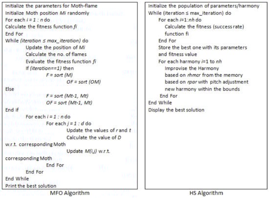
Figure 1.
Pseudocode of MFO and HS algorithms.

Table 1.
Parameters and their values used in MFO and HS algorithms.
6. Numerical Illustration
The calculation of the percentage of success rate is numerically illustrated in this section. The ball bearing assembly considered by Lu and Fei (2015) [] is taken for this work. The assembly consists of three parts, namely the outer race (A), inner race (B), and ball (C). The specifications of these parts are stated below.
The range of clearance is being kept as 18–24 microns. The tolerance of dimensions of P1, P2, and P3 are directly taken from Lu and Fei (2015) []. The dimensional specifications of the ball bearing assembly considered in this work are shown in Figure 2.
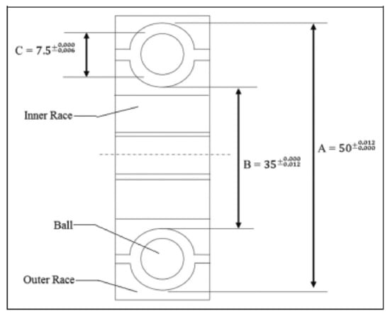
Figure 2.
Ball bearing assembly (Lu and Fei (2015) []).
The dimensional distributions of the different parts of the ball bearing assembly are given in Figure 3. It is understood from Figure 3 that each part’s distribution of ball bearing assembly is a mixture of positively and negatively skewed distribution and normal and non-normal distribution. The existing methods proposed in the past literature are not suitable to make a greater number of assemblies for this type of distribution. Hence, the novel EAUB method proposed in this work is tried out to attain a high success rate in making assemblies.
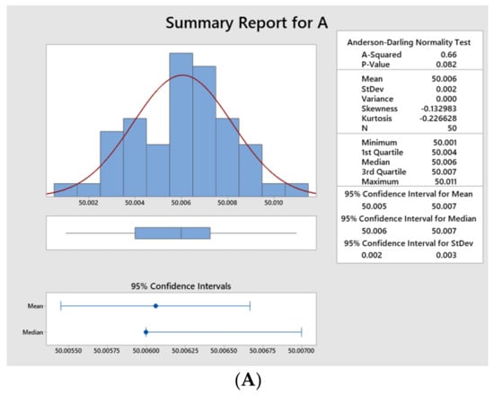
Figure 3.
Dimension distribution of parts of ball bearing assembly. Part (A)—negatively skewed normal distribution; Part (B)—positively skewed normal distribution; Part (C)—negatively skewed non-normal distribution.
For demonstration purposes, it is assumed that parts A, B, and C are partitioned into 4, 4, and 3 groups, respectively. The length of the combination of bins (L) is calculated using Equation (1) as 12 by assuming a zero arbitrary constant (E) value. Table 2 represents the number of parts available in each bin. The dimension of each part available in the bin numbers is listed in Table 3, Table 4 and Table 5 for parts A, B, and C, respectively.
Table 2.
Number of parts in each bin.
Table 3.
Dimensions details of Part A in each bin.
Table 4.
Dimensions details of Part B in each bin.
Table 5.
Dimensions details of Part C in each bin.
The duplication of bin numbers for each part is calculated using Equation (3). For demonstration purposes, the duplication of bin number 1 for part A is calculated and it is given below. The combination of bins for each part is constructed by filling the number of duplications of bin numbers and it is presented in Table 6.
Table 6.
Construction of combination of bins.
The permutations and combinations of the above are considered as a population of moth–flame and one such moth–flame representation is shown in Table 7.
Table 7.
Combination of bins.
For demonstration purposes, the assemblies are made using the first part available in the first position’s bin numbers (3, 1, and 3) in the combination of bins, which is shaded in Table 6. The number of parts and the dimension of parts A, B, and C for the corresponding bin numbers 3, 1, and 3 are presented in Table 8. For each part A, B, and C, the part is selected randomly from the bin number, and assemblies are made. The clearance value of the assembly (CLk) is calculated using Equation (4). The known lower and upper assembly clearance values are 0.018 and 0.022 mm, which are specified by the manufacturer. The calculated clearance value of 0.022 mm by assembling the first part is within the specified limits. Hence, the value of Ak will be assigned as 1. The entire CLk value for all the parts in the bin number 3, 1, and 3 of parts A, B, and C are calculated similarly and the same is presented in Table 8.
Table 8.
Calculated clearance value for the first position bin numbers.
The number of assemblies made by matching the parts corresponding to the bin numbers in the combination of the bin is shown in Table 9. The total number of assemblies made for the combination of bins mentioned in Table 7 is calculated using Equation (7) as 43. The percentage of the success rate is calculated using Equation (8) and it is 86%.
Table 9.
Number of assemblies.
The above-calculated percentage of assembly success rate is made by considering the 4, 4, and 3 bins of the parts A, B, and C, respectively. However, further analysis is mandatory to see the effectiveness of the proposed EAUB method when the number of bins of parts A, B, and C is varied. Hence, the L16 orthogonal array is used to vary the bin numbers of parts A, B, and C appropriately while making assemblies. The MFO and HS algorithms are implemented to identify the best combination of the number of bins of the parts A, B, and C for maximizing TA and the percentage of SR. The results are given in Table 10. The maximum SR value obtained through these algorithms is also highlighted. The results showed that the MFO algorithms yielded better results compared to the HSA.
Table 10.
L16 orthogonal array.
The analysis of variance (ANOVA) is carried out on the results of the MFO algorithm using Minitab v19 software for the SR value, and the details are given in Table 11. The ANOVA analysis infers that the p-value of linear, square, and two-way interaction models is less than 0.05 for SR.
Table 11.
ANOVA analysis for SR obtained using MFO algorithm.
The significance of the number of bins of each part to maximize the number of assemblies is thoroughly analyzed using the following statistical analyses. The Pareto chart and residual plot are given in Figure 4a,b, respectively. The influence of the number of bins of different parts on making the number of successful assemblies is clearly understood from these figures. From the spatial distribution (Figure 4c), it is concluded that the range of the number of bins for each part is appropriately selected. The probability plot is given in Figure 4d. It is used to verify the statistical significance of the number of bins of parts A, B, and C in increasing the success rate of making assemblies. The surface plots indicating the relationship between the number of total assemblies (TA) and the number of bins of parts A, B, and C are given in Figure 5. It is understood from Figure 5a that the TA value is gradually increased when increasing the number of bins of part A. However, when increasing the number of bins of part B, the TA value is gradually decreased. Figure 5b depicts that the TA value is slightly increased initially and then decreased while increasing the number of bins of part A. However, when increasing the number of bins of part B, the TA value is gradually decreased and then increased. The same kind of pattern is also observed in Figure 5c as in Figure 5b. Furthermore, the statistical analyses on the results of the HS algorithm are presented in Figure 6.
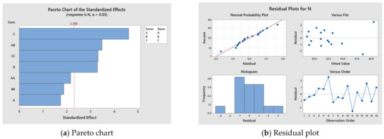
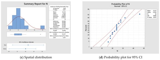
Figure 4.
Statistical analyses of the results of the MFO algorithm.
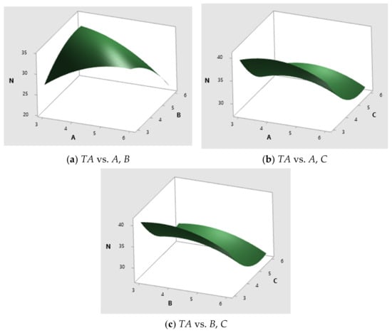
Figure 5.
Surface plots.
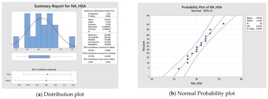
Figure 6.
Statistical analyses of the results of the HS algorithm.
Furthermore, the quadratic type multiple linear regression model (MLRM) for the number of assemblies is formulated using Minitab™ software based on the relation between the number of bins of parts A, B, and C and the output response as success rate. The MLRM is given in Equation (9).
Furthermore, in view of analyzing the statistical difference between the results of the MFO and HS algorithm, the paired t-test is conducted using Minitab software. The results such as descriptive statistics, estimation of paired difference, and the testing of significant difference are presented in Table 12, Table 13 and Table 14, respectively. The p-value from this test is less than 0.05, which stated the significant difference between MFO and HS algorithm.
Table 12.
Descriptive statistics.
Table 13.
Estimation for paired difference.
Table 14.
Testing of significant difference.
The convergence plot for both the MFO and HS algorithms based on the SR value is presented in Figure 7. From the plot, it is concluded that the MFO algorithm is quickly converged with a greater SR value when compared to the HS algorithm.

Figure 7.
Convergence plot—MFO vs. HSA.
Furthermore, the performance of these algorithms is compared through the Friedman test. The test results are given in Table 15. The sum of ranks of the MFO algorithm through the Friedman rank test is higher than the HS algorithm. Furthermore, the p-value obtained through Friedman’s ANOVA table is less than 0.05. The details are presented in Table 16. Hence, from these results, it is concluded that the MFO algorithm outperformed the HS algorithm.
Table 15.
Friedman rank details.
Table 16.
Friedman’s ANOVA table.
The optimal combinations of bins obtained through the MFO and HS algorithms as per the set of the number of bins (4, 4, 3) stated in Table 10 are given in Table 17.
Table 17.
Optimal combinations of bins.
7. Conclusions
In view of improving the percentage of the success rate of the ball bearing assembly, a novel approach called equal area and unequal bin (EAUB) numbers method was introduced in this work. The specification and tolerance value of the parts A, B, and C of the ball bearing assembly were taken from Lu and Fei (2015) []. To verify the effectiveness of the proposed EAUB method, the number of bins of parts A, B, and C were varied based on the L16 orthogonal array. The MFO and HS algorithms were used to identify the optimal combination of bins of the parts A, B, and C for maximizing the percentage of the success rate of making ball bearing assemblies. The paired t-test was conducted to evaluate the statistical difference between the results of the MFO and HS algorithms. The percentage of the success rate of making ball bearing assemblies was improved from 81.3% to 86% by using the MFO algorithm. From these results, it was concluded that the MFO algorithm outperformed the HS algorithm. This is because of good calculation accuracy, maintaining population diversity, and the quick convergence of the MFO algorithm. The convergence plot between the MFO and HS algorithms was also confirmed to be the same. Furthermore, the performance of these two algorithms was compared through the Friedman test. The optimal combination of bins of parts A, B, and C of ball bearing assembly obtained using the MFO algorithm was 4, 4, and 3, respectively.
Author Contributions
Conceptualization, S.K.M. and L.N.; methodology, L.N.; software, S.K.M.; validation, C.V. and V.K.D.; formal analysis, S.S.; investigation, H.M.A.H.; resources, H.M.A.H.; data curation, S.S.; writing—original draft preparation, L.N.; writing—review and editing, S.K.M.; visualization, L.N.; supervision, S.K.M.; project administration, S.S.; funding acquisition, H.M.A.H. All authors have read and agreed to the published version of the manuscript.
Funding
This research received no external funding.
Conflicts of Interest
The authors declare no conflict of interest.
References
- Kern, D.C. Forecasting Manufacturing Variation Using Historical Process Capability Data: Applications for Random Assembly, Selective Assembly, and Serial Processing. Ph.D. Dissertation, Massachusetts Institute of Technology, Department of Mechanical Engineering, Cambridge, MA, USA, 2003. [Google Scholar]
- Kannan, S.M.; Asha, A.; Jayabalan, V. A New Method in Selective Assembly to Minimize Clearance Variation for a Radial Assembly Using Genetic Algorithm. Qual. Eng. 2005, 17, 595–607. [Google Scholar] [CrossRef]
- Kumar, M.S.; Kannan, S.M.; Jayabalan, V. A new algorithm for minimizing surplus parts in selective assembly by using genetic algorithm. Int. J. Prod. Res. 2007, 45, 4793–4822. [Google Scholar] [CrossRef]
- Asha, A.; Kannan, S.M.; Jayabalan, V. Optimization of clearance variation in selective assembly for components with multiple characteristics. Int. J. Adv. Manuf. Technol. 2008, 38, 1026–1044. [Google Scholar] [CrossRef]
- Kannan, S.M.; Sivasubramanian, R.; Jayabalan, V. Particle swarm optimization for minimizing assembly variation in selective assembly. Int. J. Adv. Manuf. Technol. 2009, 42, 793–803. [Google Scholar] [CrossRef]
- Kannan, S.M.; Sivasubramanian, R.; Jayabalan, V. A new method in selective assembly for components with skewed distributions. Int. J. Prod. Qual. Manag. 2009, 4, 569. [Google Scholar] [CrossRef]
- Wang, W.; Li, D.; Chen, J. Minimizing assembly variation in selective assembly for complex assemblies using genetic algorithm. In Proceedings of the 2011 Second International Conference on Mechanic Automation and Control Engineering, Hohhot, China, 15–17 July 2011; IEEE: Piscataway, NJ, USA; pp. 1401–1406. [Google Scholar] [CrossRef]
- Matsuura, S.; Shinozaki, N. Optimal process design in selective assembly when components with smaller variance are manufactured at three shifted means. Int. J. Prod. Res. 2011, 49, 869–882. [Google Scholar] [CrossRef]
- Raj, M.V.; Sankar, S.S.; Ponnambalam, S.G. Genetic algorithm to optimize manufacturing system efficiency in batch selective assembly. Int. J. Adv. Manuf. Technol. 2011, 57, 795–810. [Google Scholar] [CrossRef]
- Yue, X.; Wu, Z.; Tianze, H.; Julong, Y. A heuristic algorithm to minimize clearance variation in selective assembly. Rev. Tec. De La Fac. De Ing. Univ. Del Zulia 2014, 37, 55–65. [Google Scholar]
- Babu, J.R.; Asha, A. Tolerance modelling in selective assembly for minimizing linear assembly tolerance variation and assembly cost by using Taguchi and AIS algorithm. Int. J. Adv. Manuf. Technol. 2014, 75, 869–881. [Google Scholar] [CrossRef]
- Ju, F.; Li, J. A Bernoulli Model of Selective Assembly Systems. IFAC Proc. Vol. 2014, 47, 1692–1697. [Google Scholar] [CrossRef] [Green Version]
- Xu, H.-Y.; Kuo, S.-H.; Tsai, J.W.H.; Ying, J.F.; Lee, G.K.K. A selective assembly strategy to improve the components’ utilization rate with an application to hard disk drives. Int. J. Adv. Manuf. Technol. 2014, 75, 247–255. [Google Scholar] [CrossRef]
- Lu, C.; Fei, J.-F. An approach to minimizing surplus parts in selective assembly with genetic algorithm. Proc. Inst. Mech. Eng. Part B J. Eng. Manuf. 2015, 229, 508–520. [Google Scholar] [CrossRef]
- Babu, J.R.; Asha, A. Modelling in selective assembly with symmetrical interval-based Taguchi loss function for minimising assembly loss and clearance variation. Int. J. Manuf. Technol. Manag. 2015, 29, 288. [Google Scholar] [CrossRef]
- Ju, F.; Li, J.; Deng, W. Selective Assembly System with Unreliable Bernoulli Machines and Finite Buffers. IEEE Trans. Autom. Sci. Eng. 2016, 14, 171–184. [Google Scholar] [CrossRef]
- Liu, S.; Liu, L. Determining the Number of Groups in Selective Assembly for Remanufacturing Engine. Procedia Eng. 2017, 174, 815–819. [Google Scholar] [CrossRef]
- Chu, X.; Xu, H.; Wu, X.; Tao, J.; Shao, G. The method of selective assembly for the RV reducer based on genetic algorithm. Proc. Inst. Mech. Eng. Part C J. Mech. Eng. Sci. 2018, 232, 921–929. [Google Scholar] [CrossRef]
- Asha, A.; Babu, J.R. Comparison of clearance variation using Selective assembly and metaheuristic Approach. Int. J. Latest Trends Eng. Technol. 2017, 8, 148–155. [Google Scholar]
- Aderiani, A.R.; Wärmefjord, K.; Söderberg, R. A Multistage Approach to the Selective Assembly of Components without Dimensional Distribution Assumptions. J. Manuf. Sci. Eng. 2018, 140, 071015. [Google Scholar] [CrossRef]
- Hui, Y.; Mei, X.; Jiang, G.; Zhao, F.; Ma, Z.; Tao, T. Assembly quality evaluation for linear axis of machine tool using data-driven modeling approach. J. Intell. Manuf. 2020, 33, 753–769. [Google Scholar] [CrossRef]
- Mirjalili, S. Moth-flame optimization algorithm: A novel nature-inspired heuristic paradigm. Knowledge-Based Systems 2015, 89, 228–249. [Google Scholar] [CrossRef]
- Li, X.; Zhang, X.; Yin, M.; Wang, J. A genetic algorithm for the distributed assembly permutation flowshop scheduling problem. In Proceedings of the 2015 IEEE Congress on Evolutionary Computation (CEC), Sendai, Japan, 25–28 May 2015; IEEE: Piscataway, NJ, USA; pp. 3096–3101. [Google Scholar] [CrossRef]
- Li, X.; Zhang, J.; Yin, M. Animal migration optimization: An optimization algorithm inspired by animal migration behavior. Neural Comput. Appl. 2014, 24, 1867–1877. [Google Scholar] [CrossRef]
- Li, X.; Yin, M. Design of a reconfigurable antenna array with discrete phase shifters using differential evolution algorithm. Prog. Electromagn. Res. B 2011, 31, 29–43. [Google Scholar] [CrossRef]
- Li, X.; Ma, S.; Hu, J. Multi-search differential evolution algorithm. Appl. Intell. 2017, 47, 231–256. [Google Scholar] [CrossRef]
Publisher’s Note: MDPI stays neutral with regard to jurisdictional claims in published maps and institutional affiliations. |
© 2022 by the authors. Licensee MDPI, Basel, Switzerland. This article is an open access article distributed under the terms and conditions of the Creative Commons Attribution (CC BY) license (https://creativecommons.org/licenses/by/4.0/).