The Dynamic Image Analysis of Retaining Wall Crack Detection and Gap Hazard Evaluation Method with Deep Learning

Featured Application

Through artificial intelligence optical autonomous drones (UAV) can detect cracks. It avoids terrain collapse, maintains intact geographic features, and warns people to protect their lives. It can solve the neglect of human eye detection and the collapse of the geographical environment. Maintain the stable development of biodiversity.

Abstract

This study uses machine vision combined with drones to detect cracks in retaining walls in mountaineering areas or forest roads. Using the drone’s pre-collected images of retaining walls, the gaps in the wall are obtained as the target for sample data. Deep learning is carried out with neural network architecture. After repeated training of the module, the characteristic conditions of the crack are extracted from the image to be tested. Then, the various characteristics of the gap feature are extracted through image conversion, and the factors are analyzed to evaluate the danger degree of the gap. This study proposes a series of gap danger factor equations for the gap to analyze the safety of the detected gap image so that the system can judge the image information collected by the drone to assist the user in evaluating the safety of the gap. At present, deep learning modules and gap hazard evaluation methods are used to make suggestions on gaps. The expansion of the database has effectively improved the efficiency of gap identification. The detection process is about 20–25 frames per second, and the processing time is about 0.04 s. During the capture process, there will still be a few misjudgments and improper circle selections. The misjudgment rate is between 2.1% and 2.6%.

1. Introduction

Retaining walls are commonly found in deep mountains and hilly areas. Due to the passage of time, wind and sun, terrain changes, poor construction quality, and other factors, the loss of protective ability is likely to cause landslides, cracks, or significant gaps, resulting in indirect disasters. Therefore, regular or sample surveys of retaining walls must be carried out. Creating easy-to-scout methods for retaining walls and improving convenience is critical to avoiding these disasters. However, inspections are often difficult due to rough roads. If the retaining wall is photographed with a drone, machine vision is used to detect the condition of the retaining wall.

In this case, disasters can be reduced. The maneuverability of the unmanned aerial vehicle (UAV) can achieve the advantage of inconvenience [1,2,3]. With the control of the UAV electronic system, the use of neural network cooperation can even reduce hardware damage [4]. So, the ability to self-create morphing neural networks in research to generate innovative independent systems or new methods will be a growing trend. For the study, drones photographed cracks and gaps in retaining walls. Usually, retaining walls are located in mountainous areas, and the construction length of the retaining wall is very long. Using drone photography to design a neural network and automatic crack risk evaluation system with automatic analysis and detection functions will reduce waste of resources, personnel hazards, and costs and prevent disasters.

With lack of maintenance, the ground anchors will be rusted, and the retaining walls will be damaged by cracking. It destroys entire towns or roads, causing major disasters. This is due to the inability to measure quickly and efficiently, and for safety reasons, retaining walls must be inspected regularly for long-term maintenance. Otherwise, it will lead to the loss of more innocent lives. However, hillside areas are increasingly being developed. Manual and walking ruler inspections are time-consuming, laborious, and inefficient. Yet, tragedies such as the collapse of retaining walls have continued. Therefore, this work is devoted to the prediction and data analysis of the numerical study of retaining wall cracks. This study aims to develop a series of highly mobile automated crack detection and evaluation systems to automatically detect and analyze retaining wall cracks and store data through rapid quantification of dynamic images. Based on the established artificial intelligence network, the image of the gap to be detected can be automatically extracted in advance, and then the mark can be successfully removed. Results can be automatically quantified and analyzed through detailed characterization of cracks. For feature comparison, the system divides the results into two types of alarm information, safe and dangerous. It is applied to the detection of the clearance state of the retaining wall. So, it uses scientific data to return alerts corresponding to hazard levels, indicating whether the retaining wall needs maintenance. It is also a quantifiable evaluation agency system. This will be one of the research methods to prevent retaining wall damage using scientific methods.

Related studies are as follows: The combination of neural networks and drones is one of the tools to replace people’s climbing search or reconnaissance. Valid datasets include corner detection and nearest three-point selection (CDNTS), which can improve accuracy. The area under the curve (AUC) value ranges from 76% to 89.9%; its CDNTS significantly affects image classification accuracy. This dataset is generated by synthesizing images from the virtual world into the real world [5]. Virtually generated and synthesized datasets can be trained with virtual world objects and used for real-world training tasks. Soon, autonomous detection and defense through neural networks and drones will be possible. This study is also based on the idea of this small dataset to change neural network architectures: Phenomena prediction and training of cracks. With convolutional neural networks (CNNs), a single image can efficiently generate deep resampling computations and learn to replace noble UAV 3D sensors [6] and scale important data and features. The initial input image is extracted by convolution to its features for rescue. The convolution layer improves the image to obtain effective features. Therefore, it is defined in the first few layers of the model, followed by the pooling layers, pooling, and upsampling—repeat sampling to simplify computation. Finally, the fully connected layer is used for classification, and the multi-dimensional array is processed from the fully connected layer array into one-dimensional vector feature data. A feature comparison classifier achieves another method. It is based on a MATLAB cascade classifier and then uses machine vision-related algorithms to analyze target information using local binary pattern (LBP) features. The extraction algorithm extracts eigenvalues for classification [7,8]. After the first classification stage is completed, the edge feature comparison of the two environments is achieved using the target edge feature of the classification result. To test its feasibility, climbing areas or mountain barricades are tested and soil wall cracks are detected. The crack is the target to be tested. The retaining wall is checked with the drone flight path setup. The image is transmitted back in real time through the wireless camera of the system, and the integrated learning classifier analyzes the image. The position of the crack through grayscale, binarization, and other image pre-processing is determined, and then Canny edge detection is used to judge the edge difference between two different images and carry out a risk evaluation; in the process of feature comparison and classification, it is necessary to set an A stable threshold to ensure that the classification results are entirely differentiated.

The test image will calculate the similarity value for each dangerous crack in the dangerous crack sample. Since the crack edges are irregular, when the cracks in the test image are similar to those in the sample, the edges of non-hazardous cracks are relatively flat when there is a significant difference. Similar studies are also a new crack segmentation refinement algorithm that can be used for pavement crack detection for road measurement and pavement quality monitoring. Connecting narrow and short fracture sections can also track complex fractures, including viewing multiple fine branch fractures, often seen as separate fractures within a long fracture. Initially, three pre-processing steps are performed on images: Anisotropic diffusion, wavelet filtering, and morphological filtering [9]. All filtering methods can significantly reduce pixel intensity without losing crack information. These results appear to be marginally favorable. For wavelet processing, since it better preserves the original average power and maximizes the separation of crack pixels, the result is not much different from the most straightforward morphological filtering, so morphological filtering is used as feature extraction, and then crack segmentation is performed. Finally, the cracks are divided into longitudinal, transverse, or other directions according to the direction. Therefore, when choosing the connection method between cracks, it is necessary to pay attention to whether the width of the crack is greater than a certain value and whether the length is greater than a certain value. The multiple crack images in the dataset collected during the road survey can be regarded as cracks with a width greater than 2 mm and a length greater than 25 mm, and then the cracks can be connected. It maximizes the UAV’s obstacle avoidance ability and passing speed when traversing obstacles [10,11,12]. It is a visual positioning system established through the Global Positioning System (GPS) and computer vision. It changes the positioning system when traversing indoors or outdoors, enhancing detection of the surrounding environment.

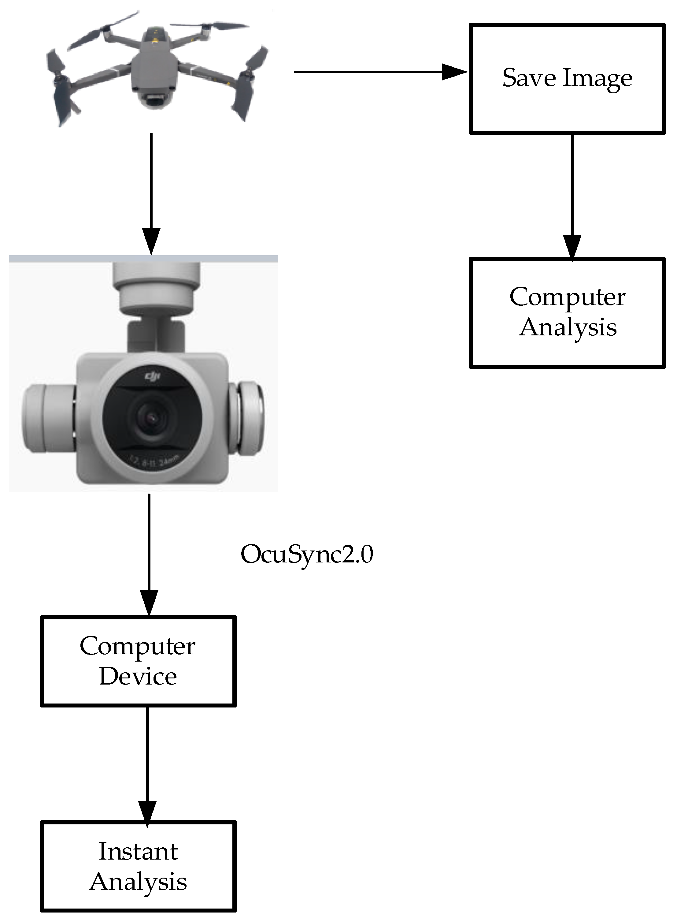
In terms of experiments, the work faced the problem of insufficient funding, and the application for research funding from the Taiwan Ministry of Science and Technology was approved. This added more equipment and team members. The drone was then equipped with a camera to film it and try to transmit the data back to the reconnaissance vehicle down the mountain. Although the computer server in the car can obtain images, the network bandwidth is limited and cannot return clear and stable images. So, after the drone returned, the pictures were uploaded to the cloud space in batches. Finally, after returning to the laboratory and downloading them to the computer, the pre-processing `parameters were changed, various regression adjustment parameters for multiple tests were selected, and the accuracy was improved. Finally, the neural network was used for deep automatic learning, and the “gap hazard evaluation method (GHEM)” and estimation model were completed. The early stages of this research are exciting because it uses data-based dynamic images to measure cracks, addressing human eye fatigue and visual errors.

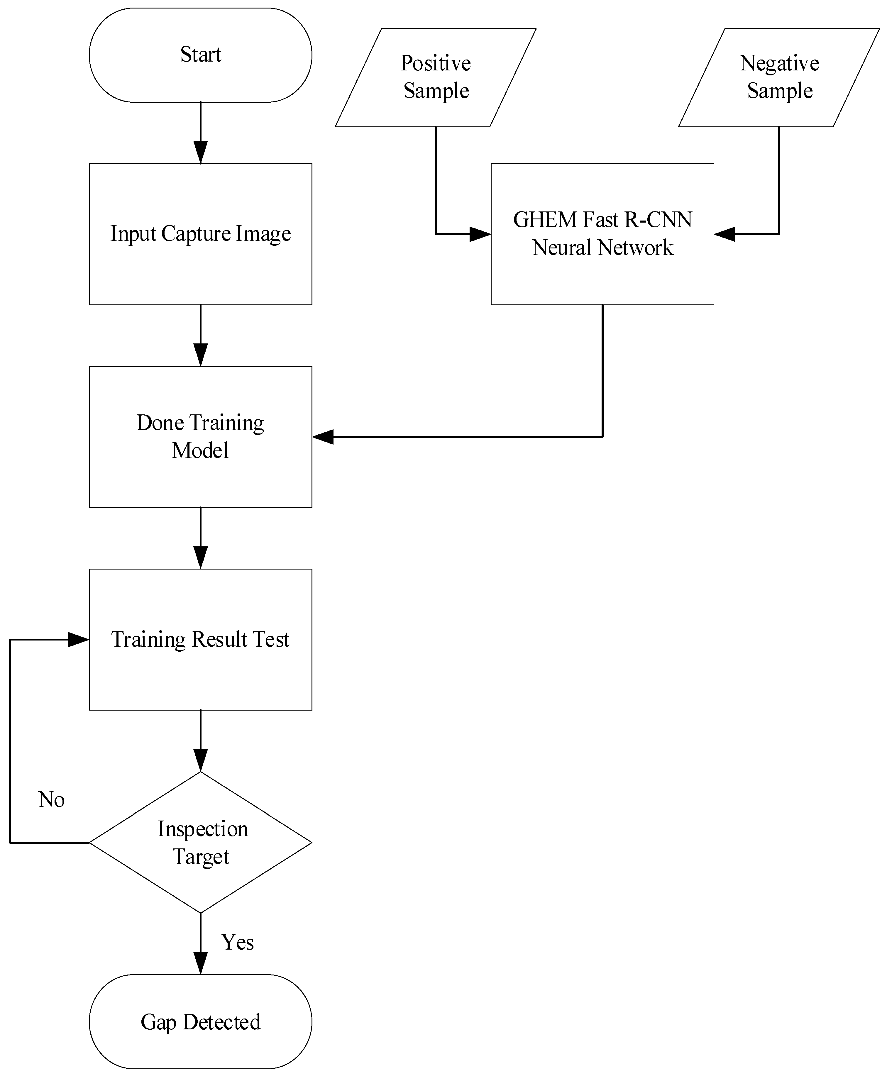
This article is outlined below. Section 1 introduces the importance of fracture features and related research; Section 2 discusses image pre/post-processing methods and the selection of neural networks. The innovative “GHEM-FastCNN” in Section 3 introduces the experimental tools and system experiment process. Section 4 is the result analysis of AI and the “GHEM” for mountain retaining wall cracks. Section 5 is the conclusion, illustrating the new value and future work of this study’s deep learning module and the GHEM.

2. Principles of The System Image Processing

Taking photos in different environments and times will affect the results of further analysis [13]. For example, the most common effects are light problems and uneven colors between objects. It is necessary to understand the color space information of the image, such as the conversion relationship between red, green, blue (RGB) and hue, saturation, value (HSV) color space, and then use color segmentation and image processing-related algorithms to achieve the purpose of detection [14].

2.1. RGB and HSV Color Space Conversion

The most common color space in life is the RGB color space. Its main principle is to apply color changes based on subjective vision. It can be divided into three variables: R, G, and B, also known as the three primary colors. The RGB color space has several drawbacks; in this color space, luminance and chrominance interact, making them very susceptible to light, which can cause uneven illumination distributions in images [15]. The most notable advantage of the HSV color space is that it can separate color and brightness in an image and can analyze color and brightness separately. The HSV color space is superior to the RGB color space in color segmentation. For example, in systems such as face detection, skin color detection, and license plate recognition, using the HSV color space as the main axis of color segmentation is recommended. The downside, though, is that computer calculations are much more expensive. Since the retaining wall was photographed in an outdoor environment and is easily affected by lighting factors, the HSV color space was also chosen in this study [16]. However, the generated image is mainly represented in RGB color space, so it is necessary to use Equations (1)–(3) to convert the image from RGB color space to HSV color space. As shown in Figure 1a, the HSV results from the pseudo-color operation improve the interpretation effect.

$$\mathrm{H}=\mathrm{aroccos}\frac{\frac{1}{2}\left(2R-G-B\right)}{\sqrt{{\left(R-G\right)}^2-\left(R-B\right)\left(G-B\right)}}$$

(1)

$$\mathrm{S}=\frac{\max \left(R,G,B\right)-\min \left(R,G,B\right)}{\max \left(R,G,B\right)}$$

(2)

$$\mathrm{V}=\max \left(R,G,B\right)$$

(3)

2.2. Morphological and Gaussian Pyramid Image Processing

The RGB image is converted into HSV space. Then, in image processing enhancement, morphology must be used first. Its basic operation definition is erosion, expansion, opening, and closing operation. It must predefine the size and shape of structural elements and then calculate each pixel value in the image. Erosion and dilation are defined in Equations (4) and (5). Opening and closing operations are Equations (6) and (7).

$$A \Theta B=\left\{ Z|{(B)}_Z\subseteq A\right\},$$

(4)

$$A\oplus B=\left\{ Z|{(\widehat{B})}_Z{\displaystyle \cap }A\subseteq A\right\},$$

(5)

$$A \circ B=\left(A \Theta B\right) \oplus B,$$

(6)

$$A • B=\left(A \oplus B\right) \Theta B,$$

(7)

where $A \Theta B$ is erosion, $A\oplus B$ is dilation, $A \circ B$ is opening operation, $A • B$ is closing operation, A is a binary image, B is a structuring element, (B)_z is the translation of the structuring element, and Z is a vector of translation.

Erosion uses the shape and size of structural elements to eliminate irrelevant pixels; dilation is usually used to fill holes in the image; opening operation means using erosion first and then dilation; closing operation is the opposite [17].

We need to segment the image. The image pyramid (Gaussian pyramid) is a kind of multi-scale representation in the image. The most important thing is to segment the image. Like the pyramid structure, the high-resolution image is in the lower layer.

The upper layer images in sequence are all $\frac{1}{4}$ of the previous layer image, so the higher the number of layers, the smaller the image and the lower the resolution. The segmentation algorithm mainly used in this study is the Gaussian pyramid, which uses Gaussian filtering to convolve the image at the current layer. As follows in Equation (8):

$$\begin{array}{c}{G}_L\left(i,j\right)={\displaystyle {\displaystyle \sum }_{m=2}^2}{\displaystyle {\displaystyle \sum }_{n=-2}^2}W\left(m,n\right)G_{i-1}\left(2i+m,2j+n\right)\\ \left(1\le I\le N,0\le i<R,0\le j<C\right).\end{array}$$

(8)

Among them, N is the number of layers in the top layer of the pyramid. R and C are the numbers of rows and columns of the first layer of the pyramid, respectively; W(m, n) represents a two-dimensional 5 × 5 function, as follows in Equation (9):

$$W=\frac{1}{256}\left[\begin{array}{ccccc}1& 4& 6& 4& 1\\ 4& 16& 24& 16& 4\\ 6& 24& 36& 24& 6\\ 4& 16& 24& 16& 4\\ 1& 4& 6& 4& 1\end{array}\right]$$

(9)

After the image passes through Equations (8) and (9) and eliminates the even-numbered rows and columns, the image of the upper quarter size can be obtained. At this time, the Gaussian pyramid of $G_0$, $G_1$,…,$G_N$ is constructed, $G_0$ is the bottom layer of the pyramid, which is the first image, and $G_N$ is the top layer of the pyramid [18,19]. After the Gaussian pyramid processes the image, although some information about the image is lost, the image information can still be recognized. Still, the layers whose resolution has been reduced, and then the subsequent analysis of crack position identification, edge detection, line detection, etc., can reduce the amount of calculation. Time and accuracy are also not affected.

2.3. Canny Detection

In general, edges are the apparent brightness changes in a collection of pixels in an image, the evolution of 1 and 0, with discontinuities. The edge part concentrates most of the information of the image and often depends on the segmentation of the image. Edges are also an essential visual feature in HSV color space images, so they are widely used in image processing and machine vision. In many studies, many scholars have proposed other edge detection methods, such as Sobel detection, Laplacian detection, etc. Sobel is a method to obtain the image stride, as shown in Equation (10). It is usually used for edge detection. It is divided into horizontal and vertical templates. The following $Gx$ and $Gy$ templates are used. $Gx$ is used to detect the vertical edge, while $Gy$ is used to detect the horizontal edge. The gradient of the pixel is obtained by the operation of the two direction templates. A gradient is a two-dimensional vector with distance and direction. The range of the distance expression varies, and the direction indicates the direction of maximum intensity.

$$\mathrm{Gx}=\left[\begin{array}{c}-1\hspace{1em}0\hspace{1em}+1\\ -2\hspace{1em}0\hspace{1em}+2\\ -1\hspace{1em}0\hspace{1em}+1\end{array}\right] \mathrm{G}y=\left[\begin{array}{c}-1\hspace{1em}-2\hspace{1em}-1\\ 0\hspace{1em} 0\hspace{1em} 0\\ +1\hspace{1em}+2\hspace{1em}+1\end{array}\right]$$

(10)

In general, in mathematical calculations, Euler distance (also known as L2 distance) is usually used, and the calculation method is the square, as follows in Equation (11).

$$G=\sqrt{G_x{}^2+G_y{}^2}$$

(11)

Since the above Equation (11) contains the square sum root sign in image processing, it is time-consuming to calculate, so the sum of absolute values (L1 distance) is usually used. The sum of absolute values is also used in the Sobel function of OpenCV as follows in Equation (12).

$$G=\left|Gx\right|+\left|Gy\right|$$

(12)

The methods of Laplace and Sobel are very similar. Both are based on the edge detection algorithm. The ideal result can be minimal only when the noise is minimal, or the smoothing filter is used to suppress the noise first. In edge detection, the noise is stopped, and the edge is accurately positioned. It is not easy to satisfy both at the same time. Removing noise through smoothing and filtering also increases the uncertainty of edge positioning. While improving the sensitivity of the edge detection operator to edges, it also increases the sensitivity to noise.

Canny is also suitable for anti-noise and precise positioning. The steps of Canny detection are as follows: The detection operation is mainly based on the first and second derivatives of the image intensity, but the derivative can easily affect the noise. The Gaussian filter, as in Equation (10), smooths the image and reduces noise [20]. To avoid the influence of noise on the detection result, Equation (13) is used.

$$H_{i,j}=\frac{1}{2\pi {\sigma }^2}{e}^{-\frac{{\left(i-k-1\right)}^2+{\left(j-k-1\right)}^2}{2{\sigma }^2}}$$

(13)

Among them, $H_{i,j}$ is a Gaussian function, taking k = 1, σ = 1, and a 3 × 3 Gaussian filter convolution kernel can be obtained as follows in Equation (14).

$$H=\left[\begin{array}{ccc}\frac{1}{2\pi }{e}^{-1}& \frac{1}{2\pi }{e}^{-0.5}& \frac{1}{2\pi }{e}^{-1}\\ \frac{1}{2\pi }{e}^{-0.5}& \frac{1}{2\pi }& \frac{1}{2\pi }{e}^{-0.5}\\ \frac{1}{2\pi }{e}^{-1}& \frac{1}{2\pi }{e}^{-0.5}& \frac{1}{2\pi }{e}^{-1}\end{array}\right] =\left[\begin{array}{ccc}0.0585& 0.0965& 0.0585\\ 0.0965& 0.1529& 0.0965\\ 0.0585& 0.0965& 0.0585\end{array}\right]$$

(14)

The gradient relationship after image smoothing is calculated. First, take the first-order differential convolution template, such as in Equation (15).

$$H_x=\left|\begin{array}{cc}-1& -1\\ 1& 1\end{array}\right| , H_y=\left|\begin{array}{cc}1& -1\\ 1& -1\end{array}\right|$$

(15)

The partial derivative of X and Y is calculated as in Equations (13) and (14), then the edge intensity and edge direction of the image, respectively, can be calculated as in Equations (15) and (16).

$$G_x\left(x,y\right)=f\left(x,y\right)*H_x\left(x,y\right)$$

(16)

$$G_y\left(\mathrm{x},\mathrm{y}\right)=f\left(x,y\right)*H_y\left(x,y\right)$$

(17)

$$G\left(x,y\right)=\sqrt{G_x{}^2\left(x,y\right)+G_y{}^2\left(x,y\right)}$$

(18)

$$\theta \left(x,y\right)={\tan }^{-1}\frac{G_y\left(x,y\right)}{Gx\left(x,y\right)}$$

(19)

Among them, $f\left(x,y\right)$s is the original image after Gaussian filter convolution, $\mathrm{G}\left(x,y\right)$ is the edge strength, and $\theta \left(x,y\right)$ is the edge direction.

The larger the value of the image gradient intensity, the more it cannot indicate that the point is an edge, and the non-maximum suppression (NMS) is used to suppress the detection along the gradient direction. The central pixel $G\left(x,y\right)$ is compared with the two pixels along the gradient line of $G\left(x,y\right)$ The gradient value of $G\left(x,y\right)$ is not greater than the gradient value of the two adjacent pixels along the gradient line. If it can be judged that this pixel is not an edge, then $G\left(x,y\right)=0$ can eliminate the relatively large gradient near the edge area. To obtain obvious and closed edges, dual thresholds are used. When the image gradient is greater than the high threshold, an image with a small number of false edges and sharper features can be obtained, but it may also make the edges unclear. First, we define two thresholds, th₁ and th₂ [19]; the relationship between the two is as follows:

th₁ = 0.4 × th₂

(20)

a. Set the gray value of the pixel whose value is less than the threshold th₁ to 0 to define this image as image 1. Set the gray value of the pixel whose value is less than the threshold th₂ to 0 to define this image as image 2.

b. Scan it based on image 2. If it encounters a non-zero pixel $p\left(x,y\right)$, continue scanning along $p\left(x,y\right)$ until the end of the contour $q\left(x,y\right)$.

c. At this time, the same position of $q(x,y$) in image 2 corresponds to a point in the same position as image 1, and its position is $\mathrm{s}\left(\mathrm{x},\mathrm{y}\right).$

d. The eight neighboring areas are centered on $s\left(x,y\right)$; if there are points with non-zero pixels in the area, let the points be $r\left(x,y\right)$, then include the position of $r\left(x,y\right)$ in image 2.

e. Then, continue scanning along with $r\left(x,y\right)$.

f. Continue to repeat steps c to e until no new contour is found in image 2.

Canny detection is used in this research because Canny detection can achieve an ideal balance between the detection effect and the time spent on the calculation compared with other edge detection algorithms [20,21].

2.4. Linear Regression

A linear regression model aims to find the relationship between one or more features (independent variables) and a continuous target variable (response variable). When the target has only a single feature, it is called univariate linear regression. Conversely, when the number of features is more than one, it is called multiple linear regression.

When building a linear regression model, it can be represented by the following Equation (21). Among them, Y is the predicted value, ${\theta }_0$ is the deviation term, ${\theta }_1$,..., ${\theta }_n$ are the model parameters, and $x_1$, $x_2$,..., $x_n$ are features.

$$Y={\theta }_0+{\theta }_1{x}_1+{\theta }_2{x}_2+\dots +{\theta }_n{x}_n$$

(21)

When training a linear regression model, the best parameters for the input data are found, and the model uses the best fit data, which is the best fit line. When there is an error between the predicted value and the observed value, the line that finds the smallest error between these errors is the best fit value line. Error is also called the residual. The residual can be visualized by observing the vertical line between the data value and the regression line. When defining the model’s error, the following Equation (22) will use the sum of squared residuals as a cost function. Among them, $J\left(\theta \right)$ is the dimensional cost function, m is the number of data items, and $\left(h(x^i\right)-y^i{)}^2$ is the residual square.

$$J\left(\theta \right)=\frac{1}{2\mathrm{m}}{\displaystyle \sum }_{i=1}^m\left(h(x^i\right)-y^i{)}^2$$

(22)

The model will complete the learning calculations through constant iterations during calculations, and iterations will increase the cost function, prompting a huge amount of calculations to reduce the learning speed of the model. Therefore, the model must reduce the dimensionality of the cost function using gradient descent. The following Equations (23) and (24) take the partial derivatives of the parameters, and all the partial derivatives can also be calculated at one time, as in Equation (25).

$$\partial J\left(\theta \right)\partial \theta 0=1\mathrm{mi}=1\mathrm{mh}\left(\mathrm{xi}-\mathrm{yi}\right)\hspace{1em}\frac{\partial J\left(\theta \right)}{\partial {\theta }_0}=\frac{1}{\mathrm{m}}{\displaystyle \sum }_{i=1}^m\left(h(x^i\right)-y^i)$$

(23)

$$\frac{\partial J\left(\theta \right)}{\partial {\theta }_1}=\frac{1}{\mathrm{m}}{\displaystyle \sum }_{i=1}^m\left(h(x^i\right)-y^i)x_1^i$$

(24)

$$\left(\theta \right)\left[\begin{array}{c}\frac{\partial \mathrm{J}\left(\mathsf{\theta }\right)}{\partial {\theta }_0}\\ \frac{\partial \mathrm{J}\left(\mathsf{\theta }\right)}{\partial {\theta }_1}\\ \begin{array}{c}⋮\\ \frac{\partial \mathrm{J}\left(\mathsf{\theta }\right)}{\partial {\theta }_n}\end{array}\end{array}\right]=\frac{1}{\mathrm{m}}{x}^n\left(h\left(x\right)-y\right)$$

(25)

After the partial derivative is completed, the parameters can be updated, as shown in Equations as (26) and (27), where α is the learning parameter. It is also possible to update all parameters at once, as shown in Equation (28).

$${\theta }_0={\theta }_0-\frac{\alpha }{m} {\displaystyle \sum }_{i=1}^m\left(h(x^i\right)-y^i)$$

(26)

$${\theta }_1={\theta }_1-\frac{\alpha }{m} {\displaystyle \sum }_{i=1}^m\left(h(x^i\right)-y^i)x_1^i$$

(27)

$$\left[\begin{array}{c}{\theta }_0\\ {\theta }_1\\ \begin{array}{c}⋮\\ {\theta }_n\end{array}\end{array}\right]=\left[\begin{array}{c}{\theta }_0\\ {\theta }_1\\ \begin{array}{c}⋮\\ {\theta }_n\end{array}\end{array}\right]-\alpha \left[\begin{array}{c}\frac{\partial \mathrm{J}\left(\mathsf{\theta }\right)}{\partial {\theta }_0}\\ \frac{\partial \mathrm{J}\left(\mathsf{\theta }\right)}{\partial {\theta }_1}\\ \begin{array}{c}⋮\\ \frac{\partial \mathrm{J}\left(\mathsf{\theta }\right)}{\partial {\theta }_n}\end{array}\end{array}\right]$$

(28)

Repeating the partial derivative and updating the parameter values until the cost function converges to the minimum value, if the value of α is too small, the cost function will take longer to converge. If α is too large, the gradient drop may exceed the minimum value, and eventually, the inversion cannot converge.

2.5. Deep Learning

Deep learning is a widely used AI training model and an algorithm in machine learning based on representational learning of data. Observations can be represented in various ways, such as a vector of intensity values for each pixel or, more abstractly, as a series of edges, regions of a particular shape, etc. While using some specific representations, it is easier to learn tasks from examples. The advantage of deep learning is to use unsupervised or semi-supervised feature learning and hierarchical feature extraction and efficient algorithms to replace manual feature acquisition.

2.5.1. Artificial Neural Network

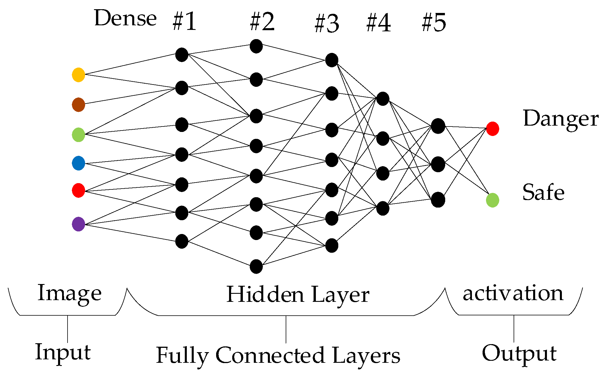
In machine learning and cognitive science, an artificial neural network (ANN) is a mathematical or computational model that simulates the structure and function of biological neural networks. It is used to estimate or approximate a function by adjusting the number of hidden layers and their density to determine the degree of generalization, thereby parameterizing the balance between efficiency and accuracy. For the classification part, an appropriate activation function can be chosen. For example, Softmax is used in this study to determine cracks’ dangerous or safe state. It is probabilistic due to the training accuracy. Neural networks perform computations by connecting a large number of artificial neurons. An artificial neural network can usually change its internal structure based on external information. It is an adaptive system. A modern neural network is a non-linear statistical data modeling tool. Neural networks are usually optimized by learning methods based on mathematical statistics. A neural network is a mathematical–statistical method with practical application. It can obtain many local structure spaces by standard mathematical and statistical methods that functions can express.

On the other hand, in artificial perception, artificial intelligence can perform artificial perception by applying mathematical statistics. This method is superior to formal logical reasoning calculus. Like the neural arrangement of the human brain, several neurons are connected to a tree. The data sampling architecture is shown in Figure 2. Each neuron is an iterative operation unit interacting with the others, and the result of the iterative operation is the training result [22].

2.5.2. Convolutional Neural Network

A CNN has always been the most important part of deep learning. A CNN can even surpass the accuracy of human recognition in image recognition. A CNN is a very intuitive algorithm. The CNN calculation process will first go through several layers of convolution operations (convolution) and several pooling layer operations (pooling). The two operations of convolution and pooling extract features from images. After feature image extraction, the system uses the full connection as a classifier [23,24], then classifies and identifies the extracted features [25], and finally substitutes the Gaussian connection to complete the neural network training.

The so-called convolution layer is the result of scanning the image through the convolution kernel (kernel), mainly to perform appropriate image enhancement on the original image so that feature points can be extracted more easily. The scanning method of the convolution kernel is shown in Figure 3.

Assuming that the image is a 5 × 5 pixel and the kernel is a 3 × 3 matrix, the corresponding operation can be performed when it is attached to the original image to obtain the result after convolution. After the image is convolved, the pixels will decrease from 5 × 5 to 3 × 3. If one does not want the original image to be convoluted and shrinking, one can first perform zero padding on the image, adding 0 around the original image to increase the original image by one order. Two circles of 0 are added to the 5 × 5 original image to convert the image into a 7 × 7 pixel image. After convolution, the enlarged image will be reduced to the original image size and will not be easily distorted.

It uses a 3 × 3 convolution kernel for edge enhancement processing in the convolution layer, as shown in the matrix in Figure 3a, so the edge enhancement convolution kernel convolves the image to be tested. It can change the affected edge points, increasing the training results’ recognition rate. Figure 4b,c are the original image and the convolved result, respectively.

2.5.3. Fast R-CNN (Regions with CNN features)

If the R-CNN is not used, but the CNN feature extraction results are used, and the two sub-operations of support vector machine (SVM) and bounding-box regression are integrated, a huge amount of calculation is generated. The operation will make the recognition rate more accurate, but it will also lead to a time-consuming operation. In addition, support vector machine (SVM) is a supervised learning method that uses the principle of statistical risk minimization to estimate the hyperplane of a classification, find a decision boundary, and maximize the boundary between the two classes, so that they can be perfectly distinguished.

Although the identification efficiency can be greatly improved, the heavy operation makes the system operation difficult. R-CNN has the following shortcomings.

(1) According to selective search, 2000 individual regions are to be extracted for each image.

(2) Extract the features of each region with CNN. Suppose that there are N pictures, then the CNN feature is N × 2000.

(3) There are three models in the whole process of target detection with R-CNN. Usually, each new surface takes 40–50 s to make predictions, so it is basically unable to handle large datasets.

The R-CNN came up with the idea of performing the CNN only once on each photo and then finding a way to do the computation in 2000 regions. In Fast R-CNN, when required, an image is fed into the CNN and the traditional feature maps are generated accordingly. Using these mappings, regions of interest can be extracted. Afterward, using an RoI pooling layer is used to rescale all proposed regions to the appropriate size for input into the fully wired network. 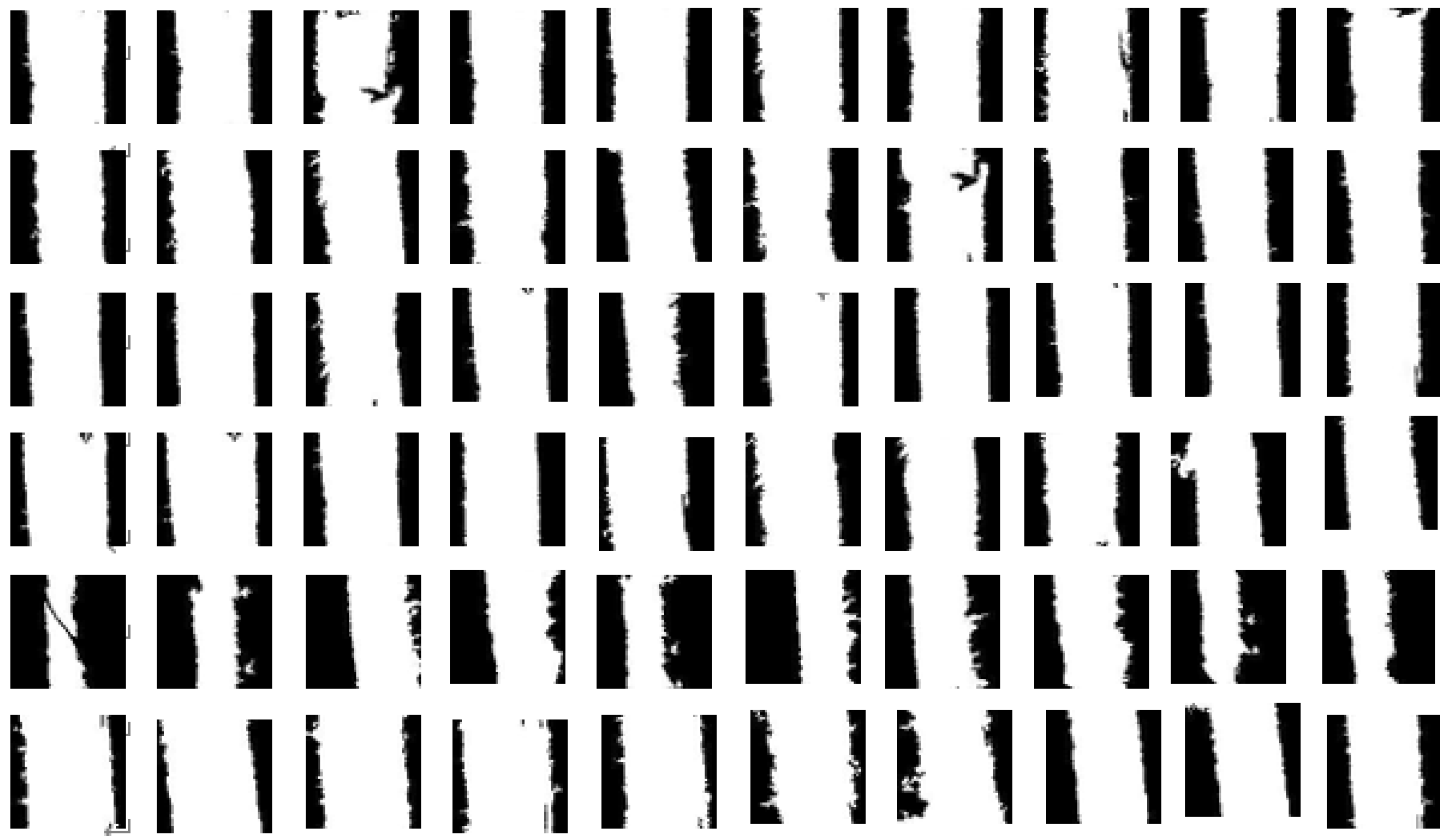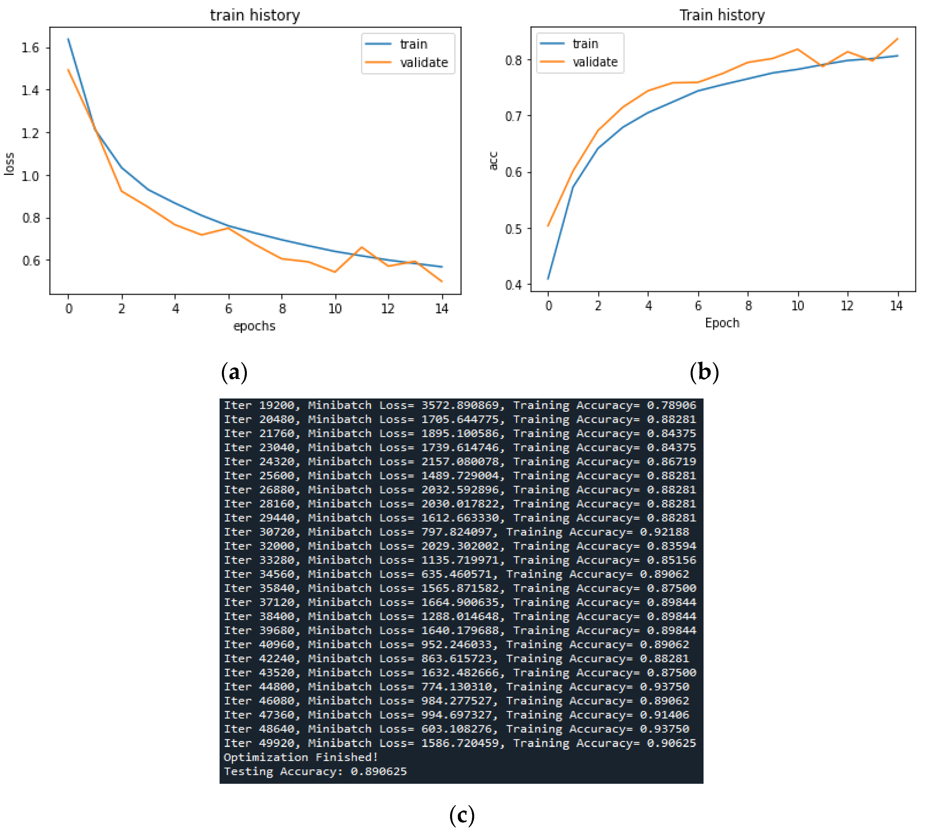Unlike the three models required by R-CNN, Fast R-CNN uses only one model to simultaneously realize feature extraction, classification, and bounding-box generation of regions [26]. The architecture is adopted in this study, and a total of 2000 dangerous and non-dangerous gap samples are input, and 50,000 iterations are performed. The batch size is adjusted to 128 units.

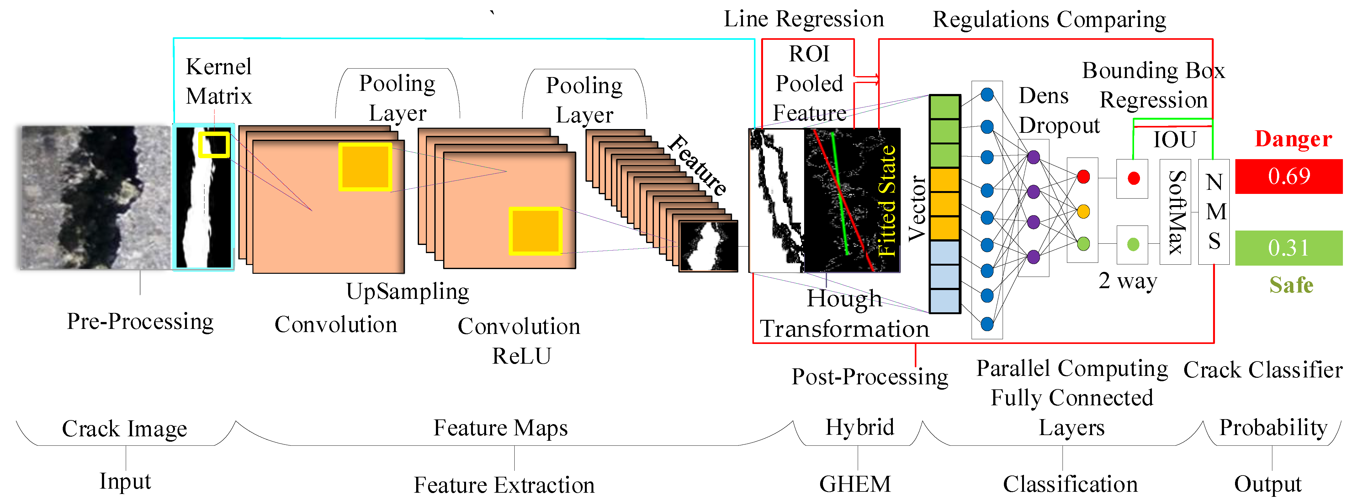
This study’s neural network system architecture is shown in Figure 5. which uses a logistic representation method by normalizing the Softmax activation function. It restricts each element to the range (0, 1) for classification effects and discovery. The sum is 1 [26], which can be enlarged to a classification probability ratio of 1 to 100%, which can also be regarded as (k-1) dimensions. NMS distinguishes between dangerous and safe objects. For example, Danger is 0.69, Safe is 0.31, and the maximum sum is 1. Among them, the regression is to find the location, and the other classification is to find the category of cracks and parallel processing simultaneously; it can make use of GPU parallel computing resources.

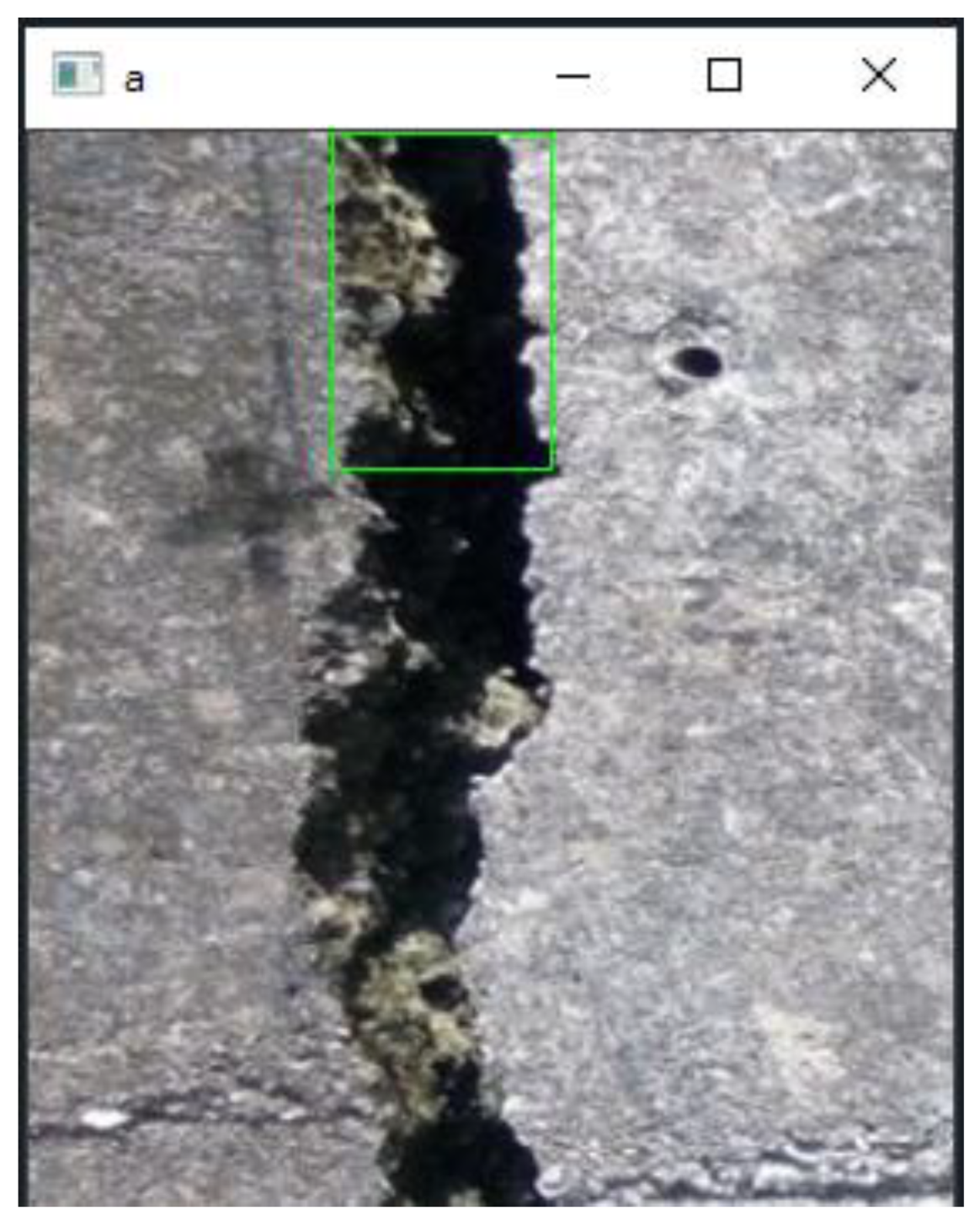
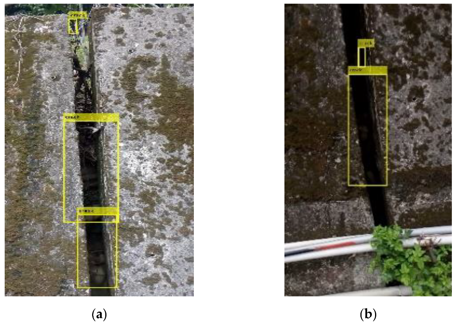
The boundary regression (bounding-box regression) is the same tool used to fine-tune the inaccurate positioning of the classifier. By saving the accurate positioning to adjust the positioning of the classifier, the feature points extracted by the classifier can be closer to the accurate value. If the green box is the ground truth of the car, the red box is the extracted region proposal. Then, even if the red box is recognized as car by the classifier due to the inaccurate positioning of the red box (IoU < 0.5), this image is equivalent to not correctly detecting the car. If that can fine-tune the red box so that the fine-tuned window is closer to the ground truth, then bounding-box regression is used to fine-tune this window. Likewise, the ground truth applied in this study is used to adjust for errors caused by seam extraction. As shown in Figure 6, the green box their relevant ground truth: In actual extraction, due to the significant gap variation or the excessive amount of feature information in the gap, position misjudgment will occur during the feature extraction process. Additional captured images are used as ground truth to adjust the accuracy of captured images.

2.6. Gap hazard Evaluation Method

After in-depth learning training [27], the feature extraction of the gap can be expected to identify the retaining wall gap effectively [28]. However, some are only expansion joints with drainage and adaptation to thermal expansion and contraction and are joints caused by damage. The potential dangers of the joints are difficult to assess. Therefore, this study also proposes the corresponding gap evaluation parameters, including the scheme to distinguish between normal expansion joints and abnormal gaps, and evaluate the conditions under which abnormal gaps may cause disasters.

The so-called expansion joint is the space reserved at the joint between two different walls. As the slope absorbs water, when it rains, the slope that absorbs water will increase the weight of the soil layer. If too much water cannot be properly discharged, the wall may fail to support the weight of the slope and collapse. Therefore, expansion joints must be designed for drainage, and expansion joints can also adapt to the volume changes brought about by thermal expansion and contraction. The expansion and contraction space must be appropriately vacated so that the wall is not easy to collapse.

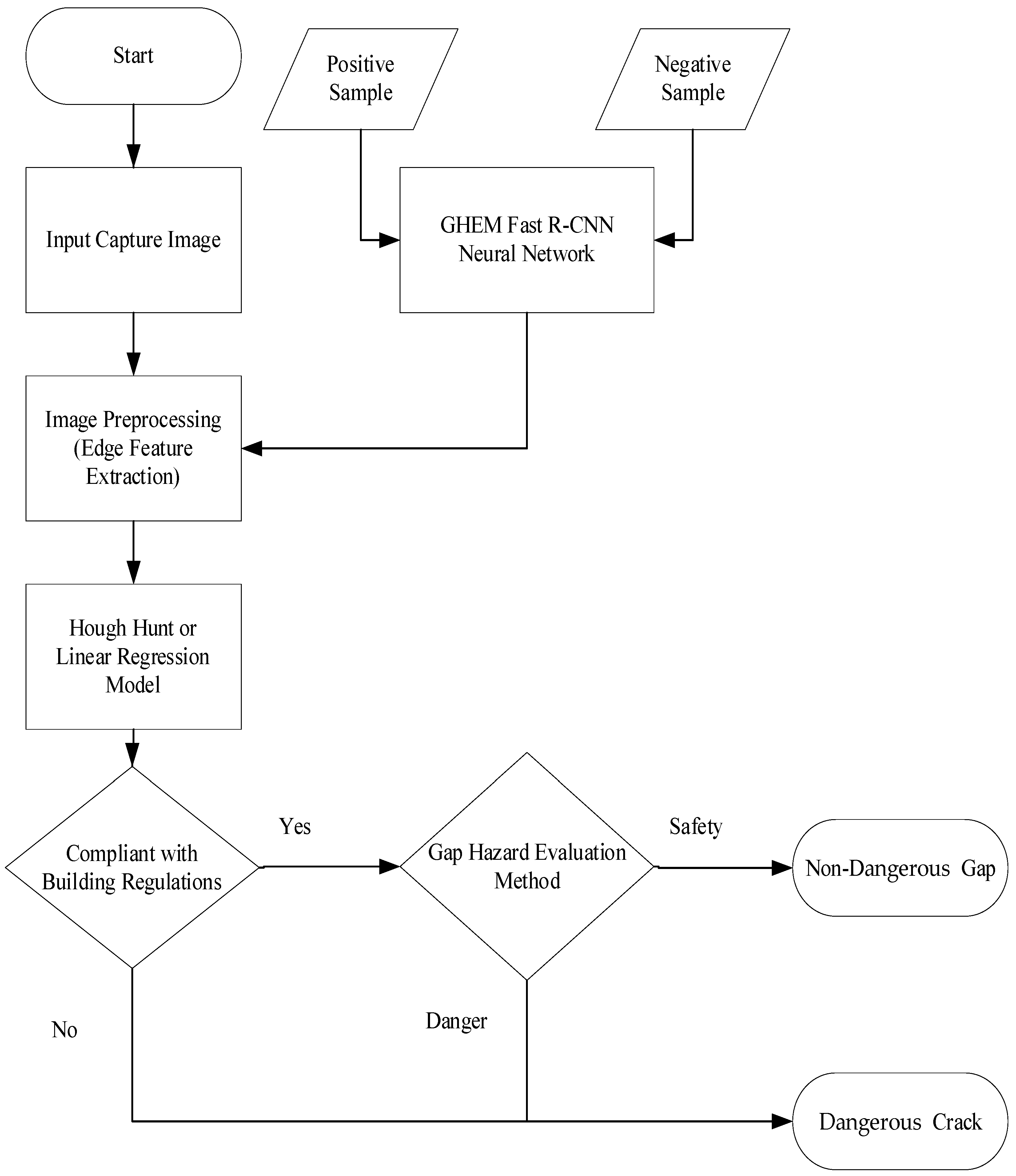
However, expansion joints belong to the category of safety gaps and must be distinguished from other gaps. According to the current building codes and regulations, expansion joints should be provided for each one-way wall, with frame structure exceeding 50 m long, and bent frame structure exceeding 60 m long. The seam width must be between 30 and 50 mm. Therefore, if the expansion joint exceeds the scope of violation of laws and regulations, there is a possibility of danger. Then, the gap width $D_n$ can intuitively show the safety of the expansion joint. In appearance, the expansion joints are relatively straight, and the width is reasonably neat. When extracting features, the relationship between line segments can be easily extracted through the Hough method of taking lines.

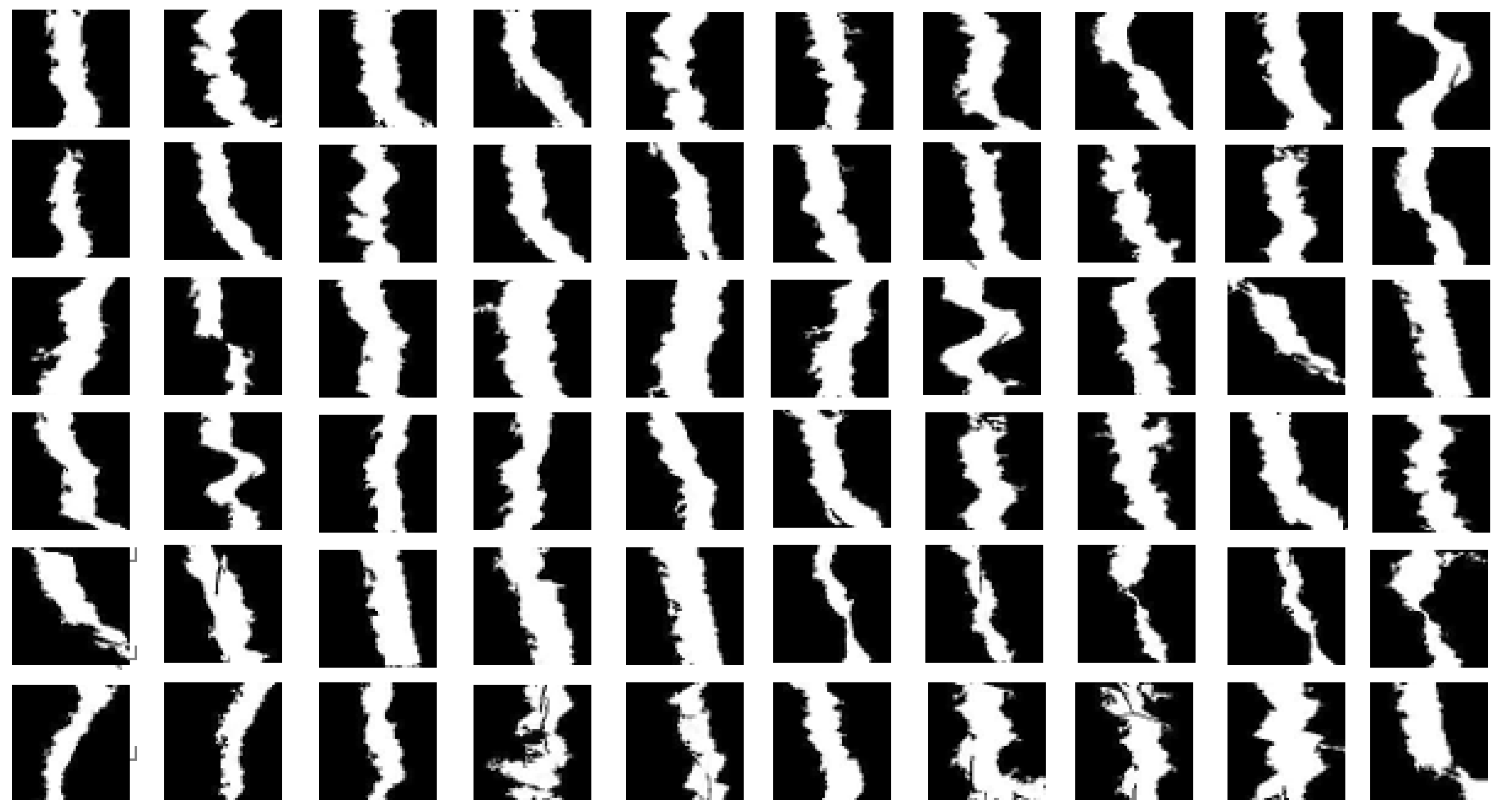
Compared with expansion joints, abnormal gaps are more irregular, with significant directional changes and large gap width variability, which will be more difficult at the evaluation level [29]. The current reference plan is based on the ratio of the gap to the wall itself and the average width of the gap for preliminary evaluation.

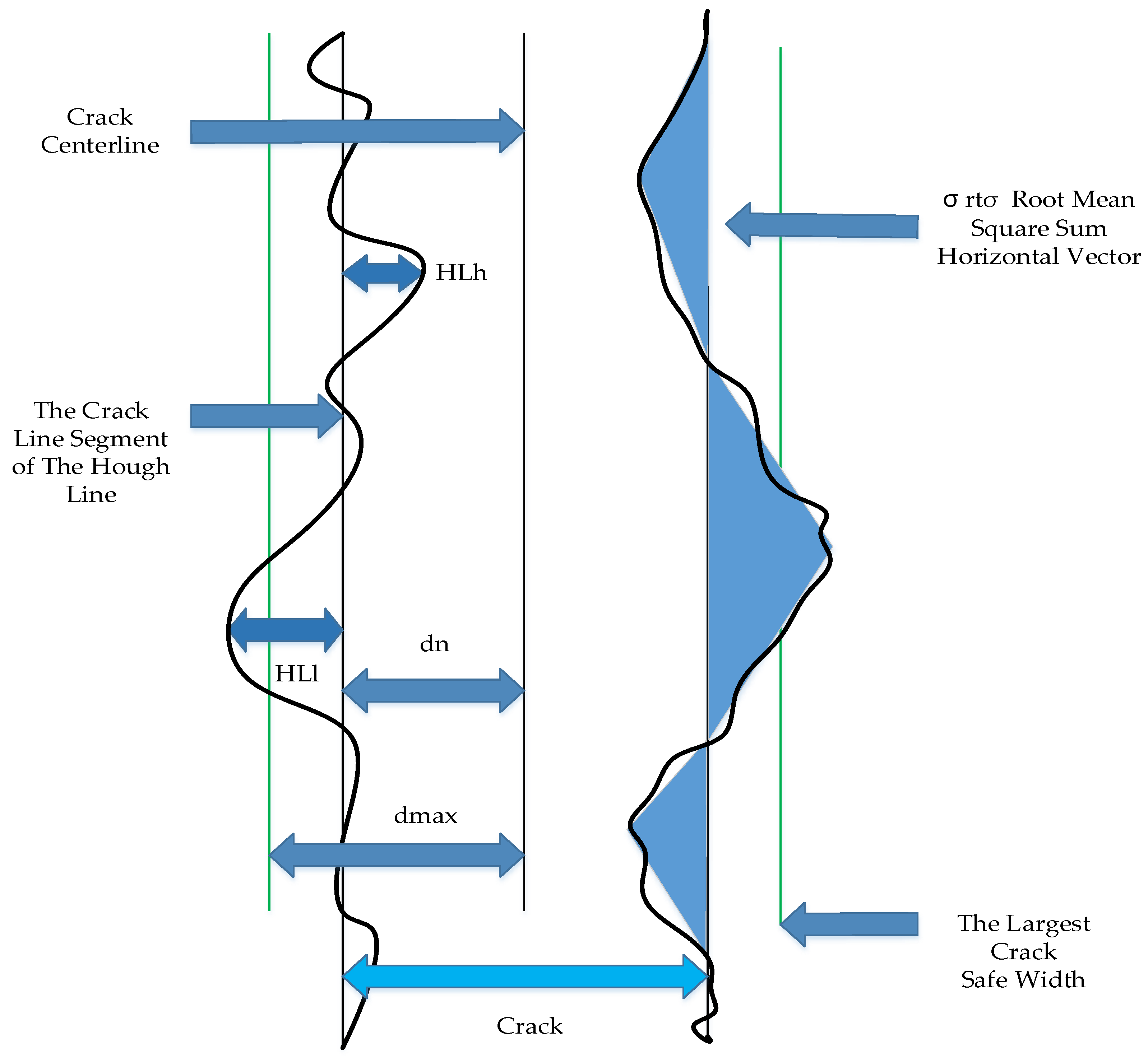
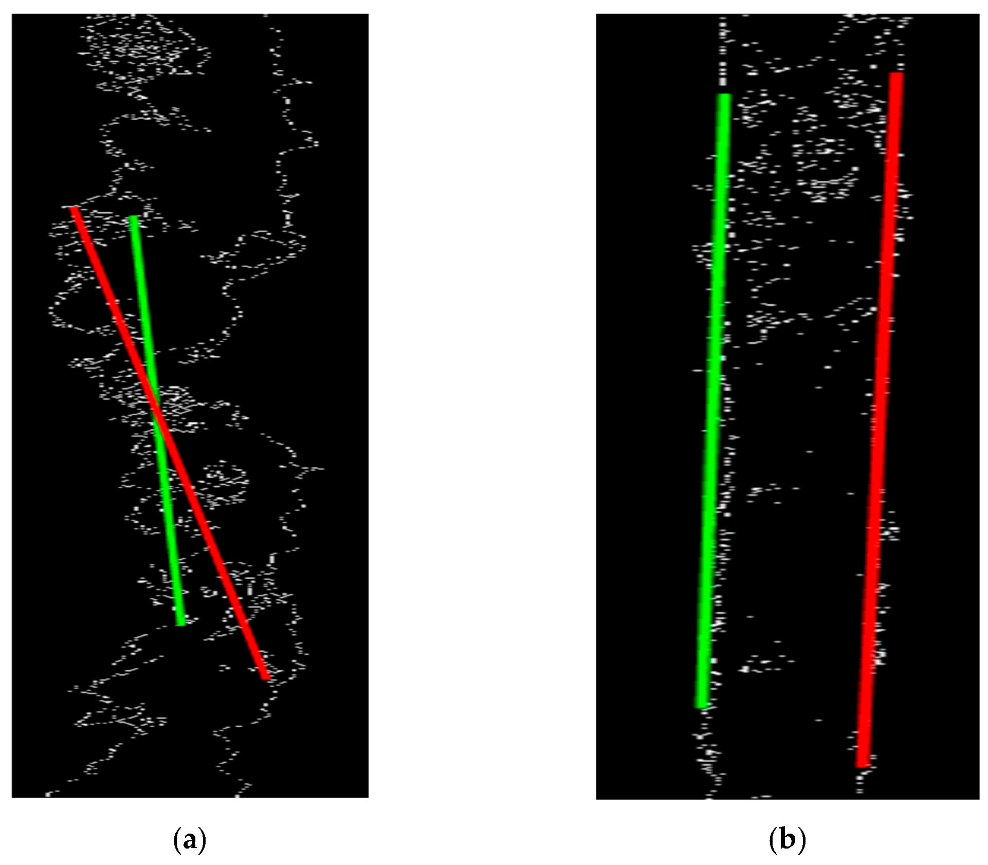
This study design takes the features extracted after deep learning as the RoI, separates the parts with gaps in the image, performs image post-processing [29], and uses linear regression modules to perform coordinate linear regression on the feature points. To find the line segment relationship in the gap that can be used for evaluation. Among them, it can be observed that the gap will mainly have two straight lines extracted, as shown in the following Equations (29) and (30), $XL$ and $YL$ are the best fitting lines extracted by linear regression of the feature points on the left after the screen is divided, $X\sigma$ and $Y\sigma$ are the residual of the actual left line segment to the fitted line. Then, the two sets are combined with the root mean square (RMS) operation, ${\sigma }_{rt}$ is the line segment’s horizontal vector, and the crack’s horizontal variability can be evaluated, where the crack as the crack line segment obtained after feature extraction is denoted as $D_n$, and the blue block is the RMS sum of the residuals of $H_{Rt}$ to the right fitted line. This is the difference area between the actual crack and the optimized line segment, which is the size of the area. The safety of the gap can be measured.

$$\sigma =\sqrt{{\left(X\sigma -X_R\right)}^2-{\left(Y\sigma -Y_R\right)}^2}$$

(29)

$$R_t=\sqrt{\frac{{{\displaystyle \sum }}_n{\sigma }_n{}^2}{n}}$$

(30)

Through the peak values $H_{Lh}$ and $H_{Rh}$ on both sides and the valley values $H_{Ll}$ and $H_{Rl}$ of the line segments on both sides, the transverse change value of the crack line segment can be calculated as follows: Equations (31) and (32), where $H_t$ is the texture fluctuation vector, which can evaluate the degree of crack texture fluctuation. The larger it is, the more significant the variation in the crack texture.

$$h_L=H_{Lh}-H_{Ll}$$

(31)

$$h_R=H_{Rh}-H_{Rl}$$

(32)

$$H_t = \frac{h_L+h_R}{2}$$

(33)

The width itself affects its safety performance. Existing regulations are an important basis for evaluation, so the shallow risk parameters of fractures can be evaluated directly by width. In Figure 7, $d_n$ is the maximum straight line distance between the two line segments after the line segment is extracted.

Parameters are added to evaluate cracks, such as those in Equation (34). Danger factor (DF) is a risk index for assessing cracks. As shown in the figure below, $D_{max}$ is the maximum safe value of the crack width. It is about 120 mm after conversion according to the specified range and regulations. According to the rule range and scale, the pixel width is about 120 pixel after conversion. $h_{max}$ is the maximum safe value for the ripple vector, and $R_{max}$ is the maximum safe value for the transverse vector. The latter two, $h_{max}$ and $R_{max}$, are analyzed by experimental data closer to theoretical safety. These three indicators constitute the evaluation of the risk index.

$$\mathrm{DF}=\frac{D_n}{D_{max}} \times \frac{R_t}{R_{max}} \times \frac{h_t}{h_{max}}$$

(34)

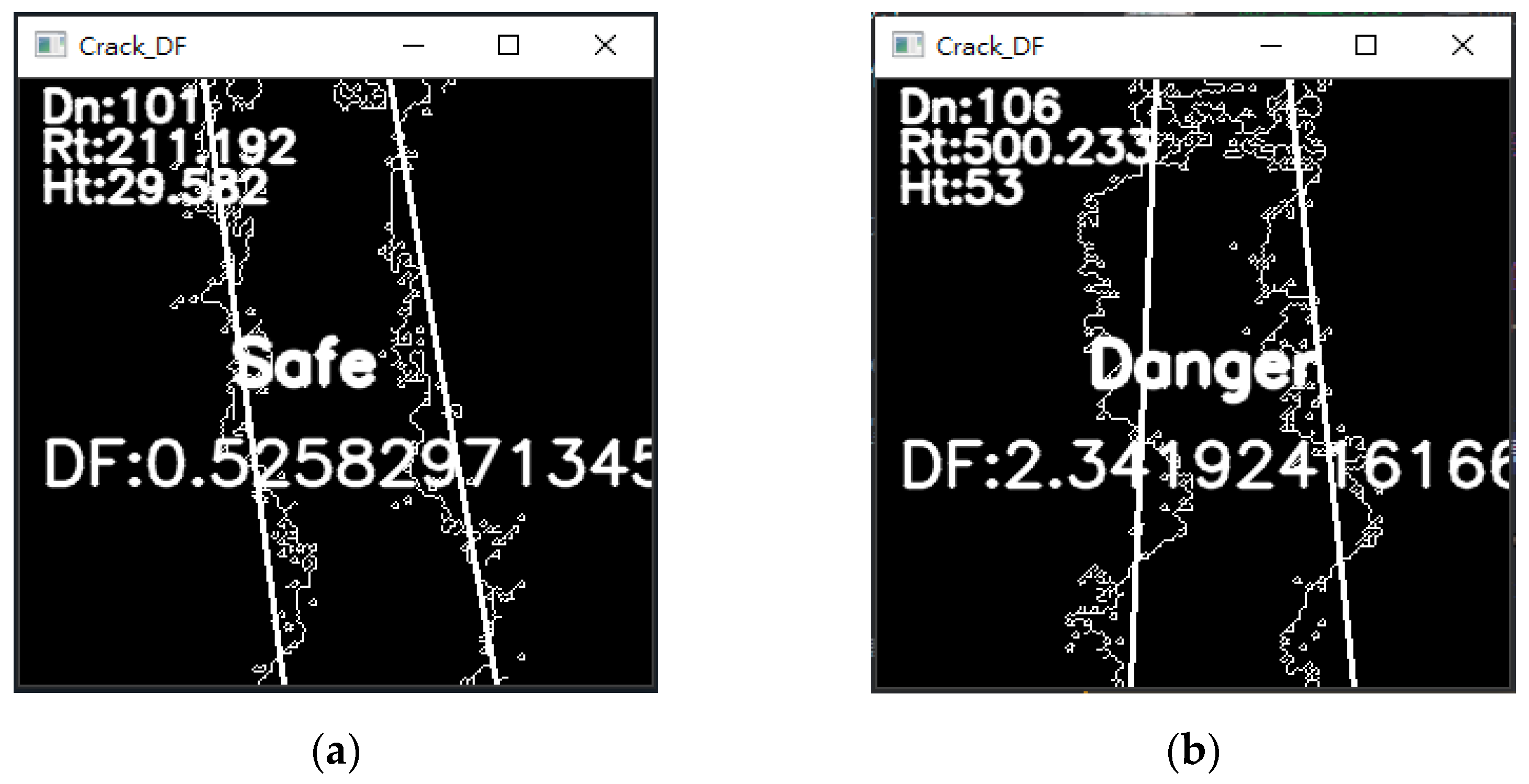
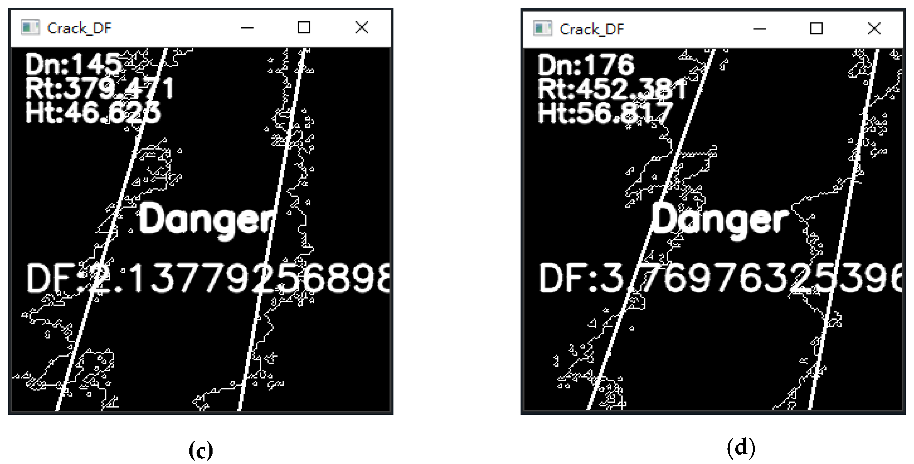
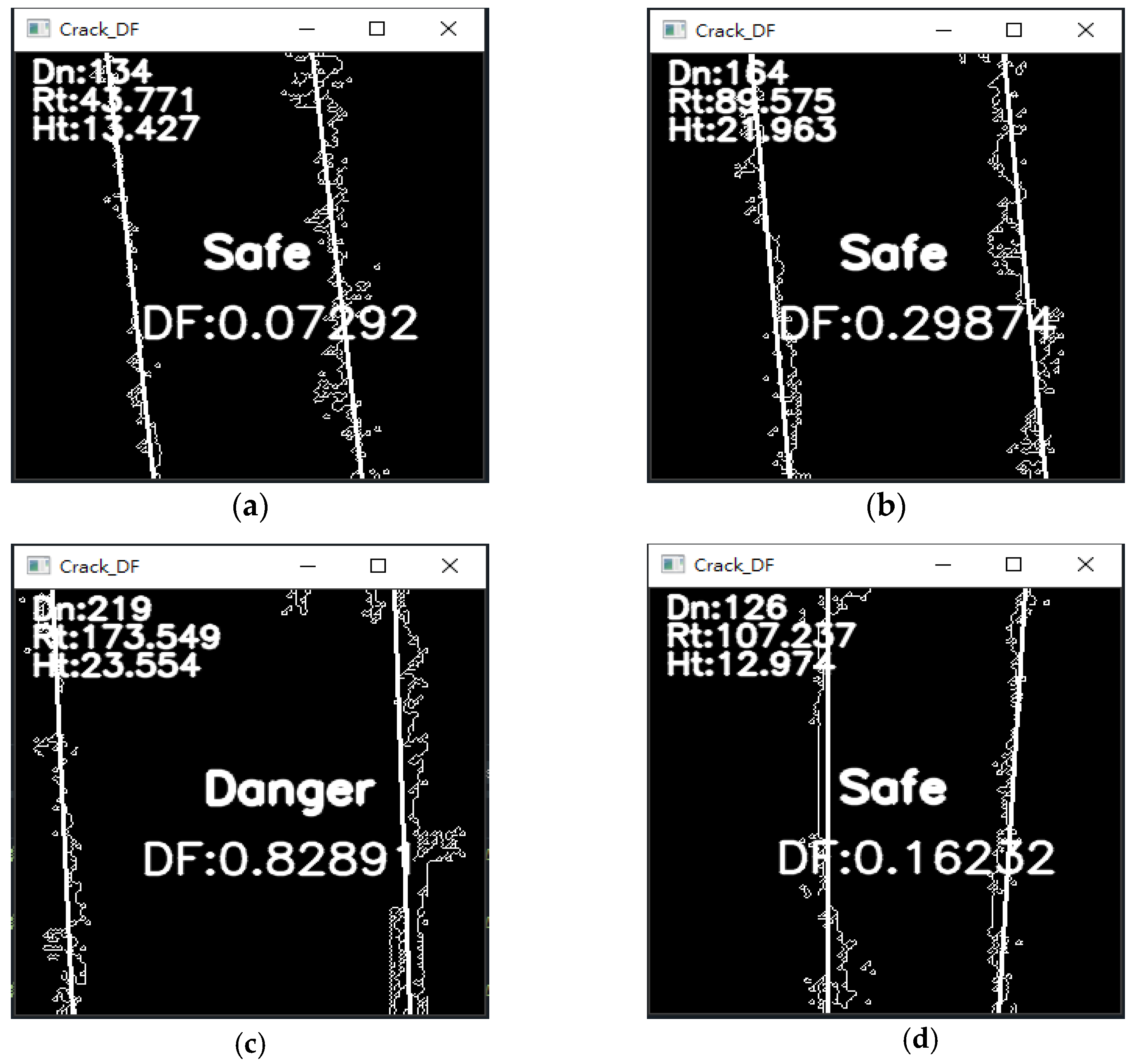
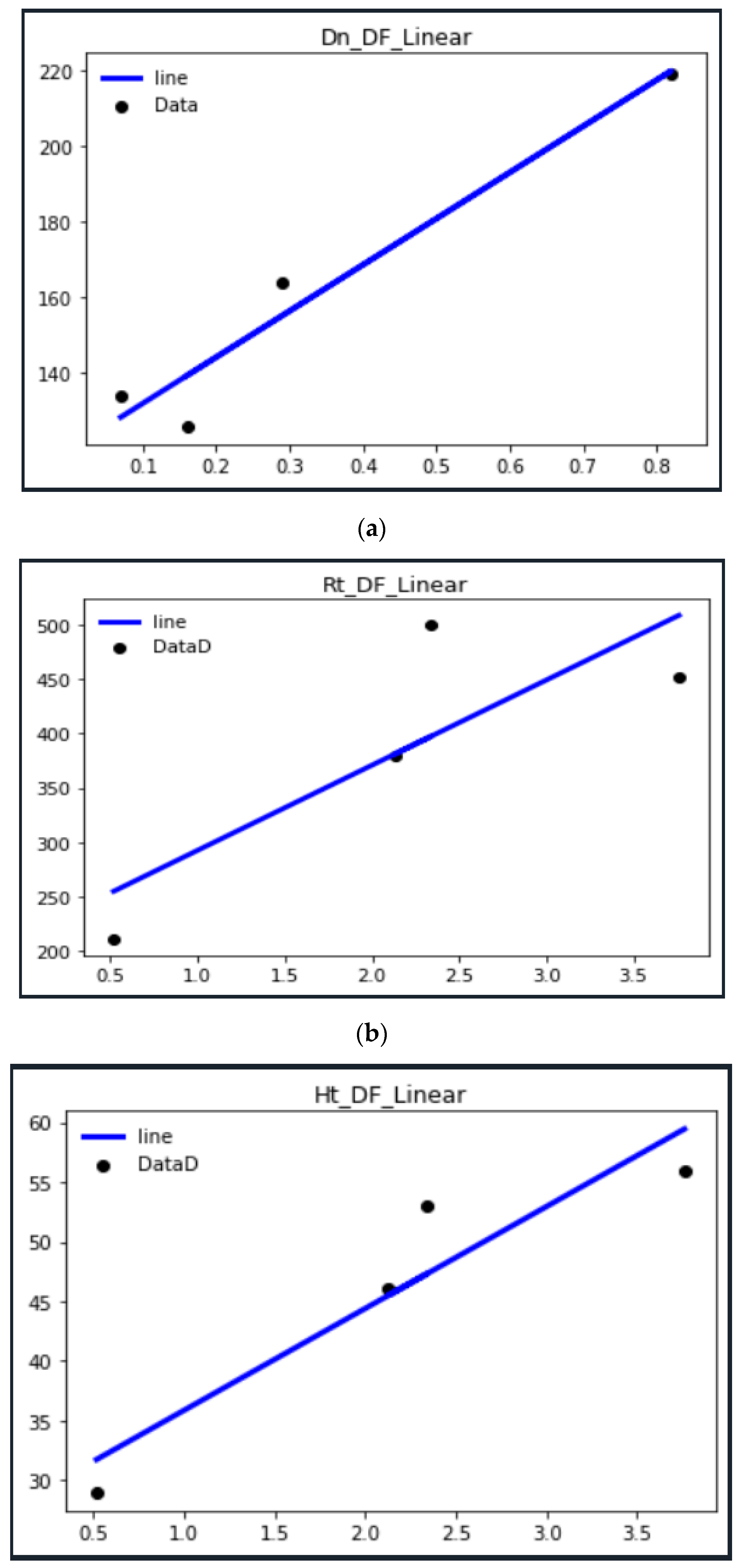
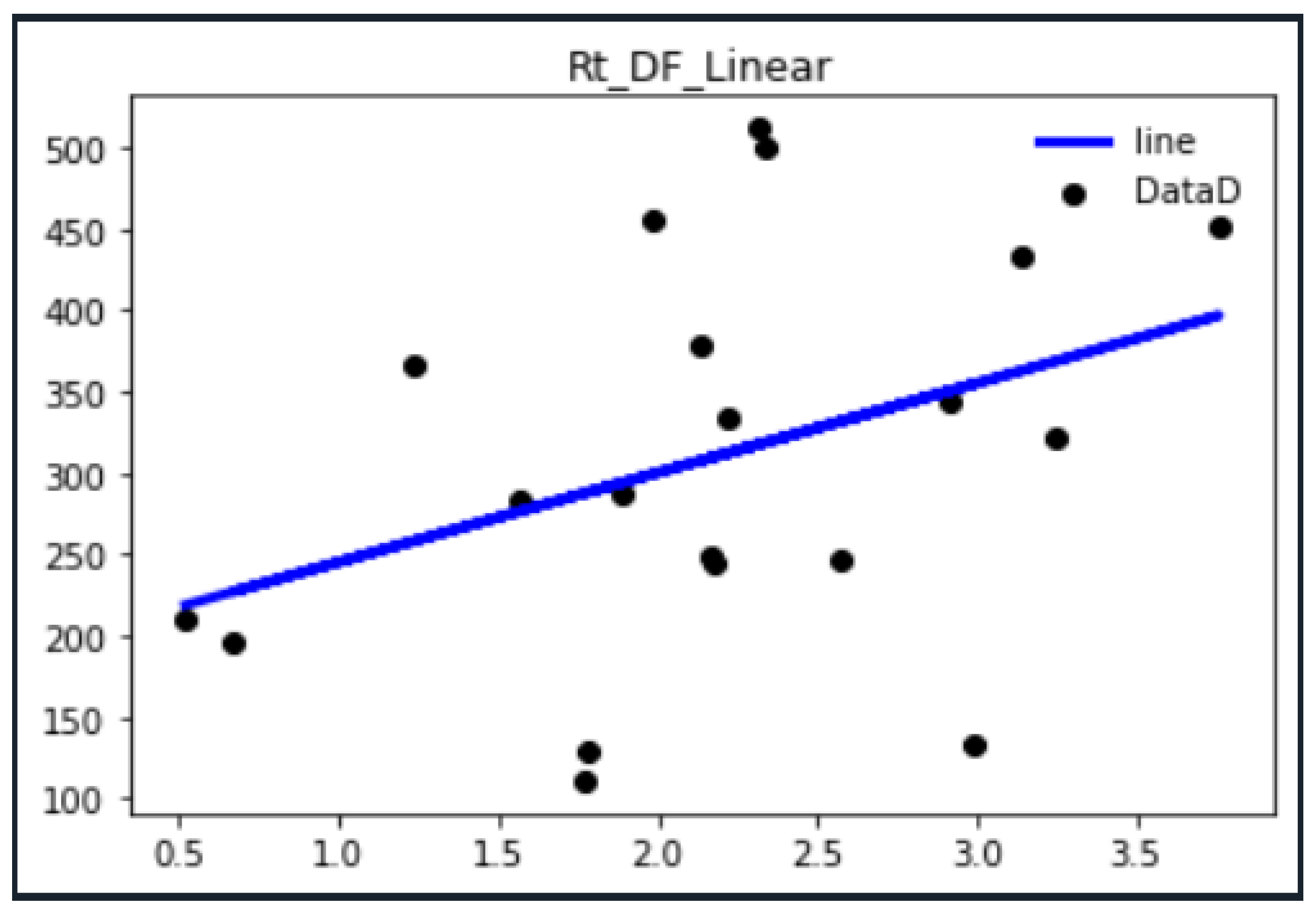
As shown in Equation (34), if the value of each coefficient is greater than its safety value, the DF will be larger, and then the risk index of the gap can be estimated. However, in the course of the experiment, it can be found that the calculated DF value between the dangerous gap and the safety gap differs by nearly a hundred times. Although obvious gaps can be used to judge safety, it is difficult to draw up an exact specification value to evaluate whether the DF value is dangerous. Therefore, in this study, weights have been added for the three indicators, as shown in Equation (35), to balance the huge difference between the two gaps and provide a DF value closer to actual safety.

$$\mathrm{DF} =fd\left(\frac{D_n}{D_{max}}\right) fr \left(\frac{R_t}{R_{max}}\right) fh\left(\frac{H_t}{H_{max}}\right)$$

(35)

Among them, f_d is the safety function of the gap width, f_r is the safety function of the projected area of the gap curve, and f_h is the safety function of the degree of undulation of the gap curve. These three weighting functions are based on the three index data collected during the experiment; linear regression is performed on the risk index DF, respectively. The best fitting line of each index is found as the weighting function. To effectively ensure that the gap hazard evaluation can better predict the crack width, the minimum crack width is measured; with the minimum distance between the 2 lines as the 2 edges of the crack, the shortest distance is the minimum crack width. To better predict the crack width and effectively ensure the gap hazard evaluation (GHE), the minimum crack width can be measured; if the distance between the two lines is the smallest, the shortest distance between the two sides of the crack is the minimum crack width. From the perspective of the model structure, it is possible to distinguish between the dangerous and non-hazardous areas, predict the crack width, and analyze it according to the danger factor of the equation. The higher it is, the more dangerous it is.

3. Experimental Architecture and Process

3.1. Software and Hardware Application and Library and Tools

The final deep learning visualization uses data from Python and Matplotlib libraries combined with Tensorflow. Python is a programming language with high object-oriented capabilities. The compilation process can bring great convenience, and it is relatively quick to modify programs or debug errors. In addition to matrix calculations and data images, Python can create human–machine user interfaces and be embedded with other development interface programs (including Matlab, Labview, etc.) to assist users in operation and data analysis. The PC hardware is I9-12900H, 16GB RAM, 3050TI 4G.

3.2. System Architecture

The aerial camera to obtain the captured image is shown in Figure 8. First, the sample images are pre-processed, and then the samples are input into the CNN neural network for training. The trained model is added into the system process to perform input recognition on the detection image, and determine whether the image is the detection target.

The neural network training and detection process is used to simulate the detection of retaining wall cracks, as shown in Figure 9. After repeated addition of sample data and weight adjustment, the gap of the target is detected and circled from the image for further safety analysis. Among them, the Fast R-CNN model is adjusted with the help of ground truth so that the detection results can avoid errors within the capture range. In the gap hazard evaluation process, each image needs to be pre-processed before sample preparation, including color space conversion, grayscale, and binarization, and then morphologically processed according to the current sample state. The apparent noise is removed. The purpose is to make the sample only have clean cracks, avoid the noise affecting the comparison process, perform feature extraction on the Canny edge, classify the initial crack position through the GHEM Fast R-CNN neural network, and further use it to extract the edge feature. Therefore, the Hough transform is utilized to extract the edge features of the target area, and a straight line component is proposed for the crack. The next step is to evaluate all line segment sets.

The evaluation process for line segments is shown in Figure 10. There are relatively few line segments, most of which are classified according to durability, and then construction joints and expansion joints are assembled. On the contrary, due to irregular cracks, the line segment collection is more complex and will be classified as irregular cracks. Among them, the safety of expansion joints must be evaluated, such as whether the crack width exceeds the construction specification. If it is not safe, it is classified as a hazardous crack from an irregular crack; otherwise, it is a non-hazardous crack.

4. Experimental Results and Discussion

4.1. Experimental Results of Cracks in Retaining Walls in Mountainous Areas

Currently, through the establishment of the database, there are 1200 samples in the hazardous clearance set and 800 samples in the non-hazardous clearance set. Figure 11 and Figure 12 show the current sample dataset (partially provided). The images in the dataset are converted into a unified format for output, and they are imported into the neural network cracks model for learning.

By importing the dataset, the number of iterations is adjusted to 50,000, the batch size is adjusted to 128 units, and the hidden layer neurons are adjusted to 256 for learning and training. The total learning time takes about 25 min. The test set is used to import the trained modules and detect the video to be tested to find the feature points in the video that meet the training results. Figure 13 below shows the test results of dangerous cracks, and Figure 14 shows non-hazardous crack videos after the test set. The box with text shows the location of the crack or expansion joint.

The FPS of the detection process is 20–25 frames, and the reaction time is about 0.04 s. The film’s continuity is still maintained, and there are still a few misjudgments and improper circle selections during the capture process. Among the 900 frames of the 30 s long film to be tested, 23 of the images are misjudged, and the misjudgment rate is about 2.555%. The improper circling range has also been adjusted by ground truth to reduce the circling error. There are slight errors in the circling of the 19-frame image with the film to be tested. The misjudgment rate is about 2.111%. In this study, single-layer convolution is used in CNN, and ReLU is used as the activation function. There are 256 neurons in the hidden layer and 10 in the output layer. Training history calculation is performed for this architecture, where the verification number is 0.2 of the original data, and 50,000 iterations are performed. The output error value is shown in Figure 15a below. As the number of iterations is small, the error value is higher, but the overall convergence to 1 is successful. The accuracy rate is also due to the insufficient number of samples and fewer iterations.

It is also observed in Figure 15b that although the accuracy rate is not high, it is gradually growing. In the future, when the number of data samples increases, the number of hidden layer neurons can be increased, and the number of iterations can be increased. As shown in Figure 15c, it is expected to grow to close to 90% of the recognition rate.

4.2. Gap Hazard Evaluation Result

After the crack feature extraction, it is necessary to classify the target and evaluate its security. In this study, the feature extraction image is converted to the Canny edge detection map, and the Hough transform is initially performed on the image to search for line segments. As shown in Figure 16, the line-finding solution for dangerous cracks and the line-hunting results for non-dangerous cracks are respectively; it can be seen that the line segment in (b) is attached to the edge of the crack so that various linear relationships of cracks can be easily observed. However, in (a), the line segment does not fit the edge of the original gap and crosses. The crossover phenomenon can only occur when the gap is tightly closed, but the gap does not have this feature. The main reason is that the Hough transformation is mainly based on the search results of the feature points according to the specific slope and length definition. The feature points in (a) change significantly, which may easily cause the judgment of unexpected results in the conversion process. Although Hough transformation cannot achieve comprehensive gap detection, it can still provide preliminary gap-related information, which has an excellent effect on the discrimination of gap forms.

Therefore, this study adopts a linear regression method to perform linear regression operations on the feature points on both sides of the gap. As shown in Figure 17, the noise points in the image are first eliminated through the open operation; then, the image is divided into left and right parts; linear regression was performed on the edge feature points, respectively. The image’s calculated line segment is redrawn based on the output coordinate points and slope. It can be observed from the results that most of the line segments of the simulation results are not parallel to each other, so when extracting the gap width value $d_n$, the maximum width of the current captured screen will be extracted.

The best fit line of linear regression is used to calculate the final indicators of the feature points, including $R_t$ and $H_t$. Figure 18 shows the indicators and evaluation results on the screen, which can more directly show the safety of the gap. The four screenshots are taken from the same dangerous gap video after calculation. (a) shows that it is possible to detect a safe result in the dangerous gap film to be tested, but the overall detection result is still the most dangerous. With the three pictures (b), (c), and (d), it can be observed in the same dangerous crack to be tested that $R_t$, $H_t$ and DF have a positive relationship, and the value of $R_t$ is large, which easily increases the growth rate of DF. The gap $D_n$ proves the dangerous gap may be small, but through the weight adjustment of its changing area and the maximum peak–valley value, the danger of the gap can be accurately detected.

The running results are counted, and are given in

Table 1. Dangerous gap evaluation datasheet.

Items	${\mathit{D}}_{\mathit{n}}$	${\mathit{R}}_{\mathit{t}}$	${\mathit{H}}_{\mathit{t}}$	DF	Security
No. 10	101	211.192	29.582	0.525829	Safe
No. 12	106	500.233	53.000	2.341924	Danger
No. 94	145	379.471	46.623	2.137792	Danger
No. 100	176	452.381	56.817	3.769763	Danger

. The collected data can calculate the weight function required by the adjustment equation. The weight function can achieve good adjustment results in the system. It can be observed that the dangerous DF value in the table is approximately between 1 and 4. The primary influence on the increase in DF are $R_t$ and $H_t$; they have a positive relationship with DF. The best fit line after linear regression calculation will reduce the influence of the two indices on the DF, and the slope of the fit line can be added to the equation as a weight function. $D_n$ is the safety width stipulated by laws and regulations, which is an inherently accurate index, so its weight should be increased to make the index occupy a more significant proportion of the system.

In contrast, importing a non-dangerous gap video can result in Figure 19. It can also be observed that Figure 18c is different from other pictures and is judged to be a dangerous state. Compared with the particular situation, Figure 19 finds that the DF value is less than the standard value 1, which in theory should be safe but is evaluated as dangerous by the system. The main reason is the influence on the $D_n$ index because the judging standard of $D_n$ is based on the current regulations, and the expansion joints of the building wall should be designed to be 30~50 mm. The length conversion corresponds to about 120~200 pixels in the evaluation system. It violates building regulations when $D_n$ is more significant than 200 pixels. No matter what the DF evaluation value, it must be considered a dangerous state. In Figure 19, three pictures, (a), (b), and (d), can be observed from the same hazardous non-crack film to be tested. $D_n$ has a positive relationship with DF, and the value of $D_n$ is more significant, which quickly increases the growth rate of DF. It proves that the changing area and maximum peak-to-valley value of the non-hazardous gap may be small, but through the weight adjustment of the gap size, the danger of the gap can be accurately detected.

The weight function can be obtained by a fitting line, as shown in Figure 20, the linear regression fitting diagram of the three indices to DF, respectively, and each datapoint is input into the model to perform linear regression on the data, where the line is the fitted line and point is the input data. Substituting the data in Table 1 and

Table 2. Non-dangerous gap evaluate datasheet.

Items	${\mathit{D}}_{\mathit{n}}$	${\mathit{R}}_{\mathit{t}}$	${\mathit{H}}_{\mathit{t}}$	DF	Security
No. 26	134	43.771	13.427	0.07292	Safe
No. 57	164	89.574	21.963	0.29874	Safe
No. 67	219	173.549	23.554	0.82891	Danger
No. 76	126	107.237	12.974	0.16232	Safe

above, the slope after fitting can be used as a weight function. Figure 20a is the process for fitting $D_n$ data Figure 20b for fitting $R_t$ data, and Figure 20c for fitting $H_{t }$ data. Then, the weight function is fed back to the system equations to make the calculation result of the equations more stable.

Enlarging the number of data entries can fit a weight function closer to the theoretical value, as shown in Figure 21, by increasing the $R_t$ data to 20, and obtain a more accurate weight function through the convergence of the fitting line. The same $D_n$ and $H_{t }$ can also similarly converge to the best weight function.

There are not many data and, in order to solve the problem of small datasets for deep learning, this study makes it more stable by fitting. After repeatedly superimposing data and linear regression, the slope of the fitted line segment will also converge to stability with more data and then be used for weight adjustment. The final DF value should converge in the direction of 1, as given in Table 2 below. It can be observed that the DF value combines as expected under the same value, making the DF value closer to the accurate value.

5. Conclusions

In this study, a total of 2000 samples of hazardous and non-hazardous gaps were input from the system for 50,000 iterations. The batch size was adjusted to 128 units. Effective accuracy of 89.06% can be obtained through model training. When people go to deep mountains or slopes for inspection, they must stand above or below the retaining wall and use a ruler to inspect visually. Often restricted by terrain, it is not easy to judge. Comparing the experimental and predicted results of crack width measurement, the difference is less than 1.5%. However, the overall measurement is performed with certainty, thus avoiding human error or oversight and uncertainty. This study implements a Fast R-CNN-based deep learning module and the “gap hazard evaluation method (GHEM).” The expansion of the database effectively improves the efficiency of gap recognition, and the post-processing and feature extraction of the segmented images have achieved good results. The weight function is obtained by linear regression of the data and is used to adjust the unreasonable weight distribution in the equation to make the system more stable. The detection process is about 20–25 frames per second, and the processing time is about 0.04 s. In capturing packets, there will still be errors in judgment and improper circle selection. The false positive rate was between 2.1% and 2.6%. Although deep learning architectures effectively extract the components of seams in images, their efficiency is not maximized; when combined with the innovative “gap hazard evaluation method,” unreasonable false positives can be more effectively avoided. If used for real-time detection, time-consuming or low frame rate contour image recognition may be encountered. The complete database and weight distribution can be adjusted to give the module better recognition efficiency, or other neural network architectures can be tried to improve the deficiencies of existing modules.

Regarding the system, in the methods of the GHEM Fast R-CNN, this work is performed on the entire system, and pre-processing is performed first. On the basis of Fast R-CNN, CNN, and ReLU resampling, feature points, and line regression are added to enhance processing and the GHEM. This system finally uses Softmax as an activation function and NMS, which can detect cracks more effectively.