Occupancy Reward-Driven Exploration with Deep Reinforcement Learning for Mobile Robot System

Abstract

This paper investigates the solution to a mobile-robot exploration problem following autonomous driving principles. The exploration task is formulated in this study as a process of building a map while a robot moves in an indoor environment beginning from full uncertainties. The sequence of robot decisions of how to move defines the strategy of the exploration that this paper aims to investigate, applying one of the Deep Reinforcement Learning methods, known as the Deep Deterministic Policy Gradient (DDPG) algorithm. A custom environment is created representing the mapping process with a map visualization, a robot model, and a reward function. The actor-critic network receives and sends input and output data, respectively, to the custom environment. The input is the data from the laser sensor, which is equipped on the robot. The output is the continuous actions of the robot in terms of linear and angular velocities. The training results of this study show the strengths and weaknesses of the DDPG algorithm for the robotic mapping problem. The implementation was developed in MATLAB platform using its corresponding toolboxes. A comparison with another exploration algorithm is also provided.

1. Introduction

In the past two decades, an enormous number of works on the mobile-robot exploration domain or the so-called mapping or map coverage have been published [1,2]. Generally, every novel exploration technique aims to solve three basic challenges. The first is to explore fully a given space using an onboard robot-vision system. The second is to not encounter any obstacles while driving through. The next is to optimize the driving course in the exploration, saving time and energy costs. This represents a bigger picture of mapping, addressing only problematics.

Delving deeper into the field, various characteristics of an exploration can be discovered. For instance, for environment types, the exploration can be conducted indoors, outdoors [3], on cluttered rough terrain [4,5], in a post-disaster extreme environment [6], in the ocean [7], or on a planetary surface [8]. The exploration can have requirements based on the map type (grid map [9], octomap [10], point cloud map [11], semantic map [12]) or the approach (deterministic [13,14], stochastic [15], artificial intelligence [16,17], SLAM- (Simultaneous Localization and Mapping) type [18,19]). In addition, the exploration can be processed by different robot systems [20]: a mobile-robot system or multi-robot system. These various characteristics are the reasons why mapping the field is an important topic in robotics and why it remains relevant today.

In mobile-robot exploration, a robot is launched into a space with entirely unknown information about the indoor environment. A robot can have vision using a sensor or camera that senses at a certain sensing distance or image resolution, respectively. During mapping, the robot drives towards and perceives more knowledge about the environment. It can have a task or an action command while it moves in the environment. The task can be a point in the environment, which is called a local point or a waypoint [21]. The computation of the waypoints in the mapping is conducted by a computational algorithm, which many scholars have attempted to either modify in combination with other techniques or create new ones. In this study, the exploration does not use the waypoint concept. Instead, the robot moves by following the action command being transmitted to the robot motors.

The final result of the robotic exploration is a finite map. The map is a data model of the robot’s surroundings. The robot needs the map on a regular basis to have knowledge of its position for further missions. Object recognition, object segmentation, planning movement, and many other typical human activities in indoor space are required for an existing known map, which is true for a robot as well.

Artificial intelligence (AI) is a significant topic in science nowadays [22]. It is believed that AI is a general term, which describes how computers or hardware systems can think and behave like a human. A subfield of AI is machine learning [23]. It is mainly focused on learning from data training. Over decades, machine learning evolved into deep learning, which could transform the data into multiple-layer representations due to feature detection or pattern classification [24]. The considerable success of some applications, such as image recognition, speech recognition, email spam filtering, and the winning of AlphaGo in the board game Go, motivated developers around the world to apply machine learning or deep learning techniques in various fields.

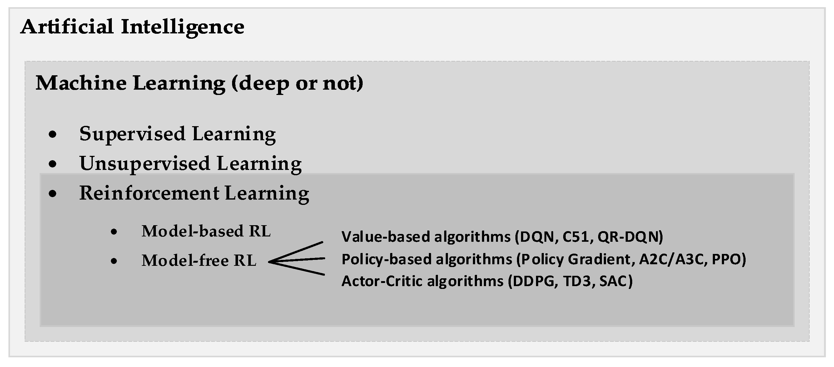
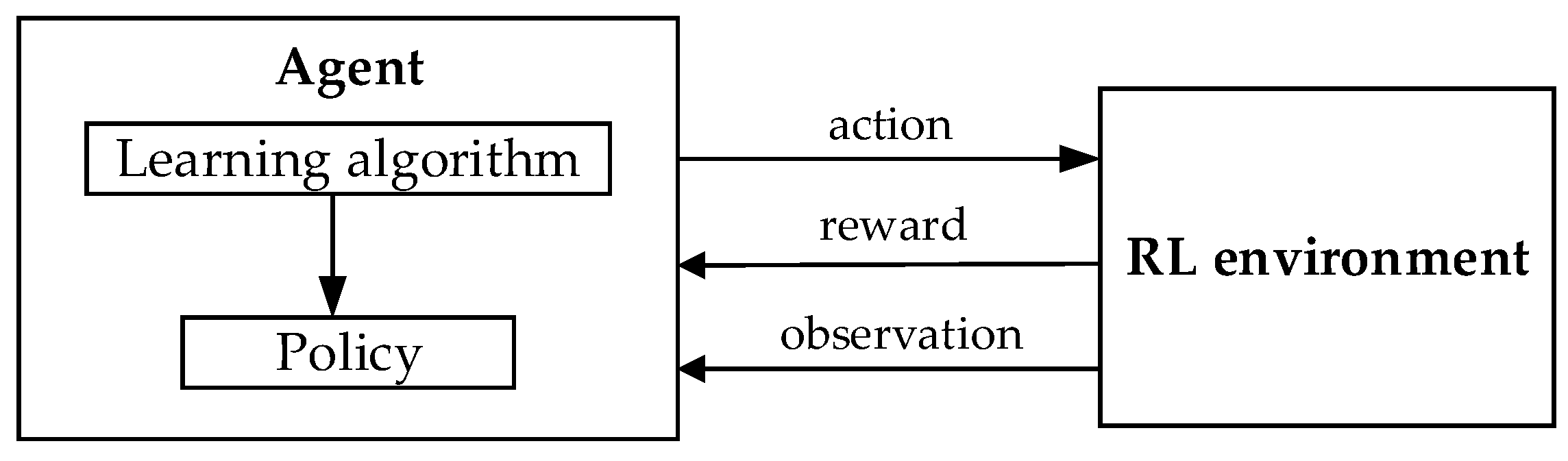
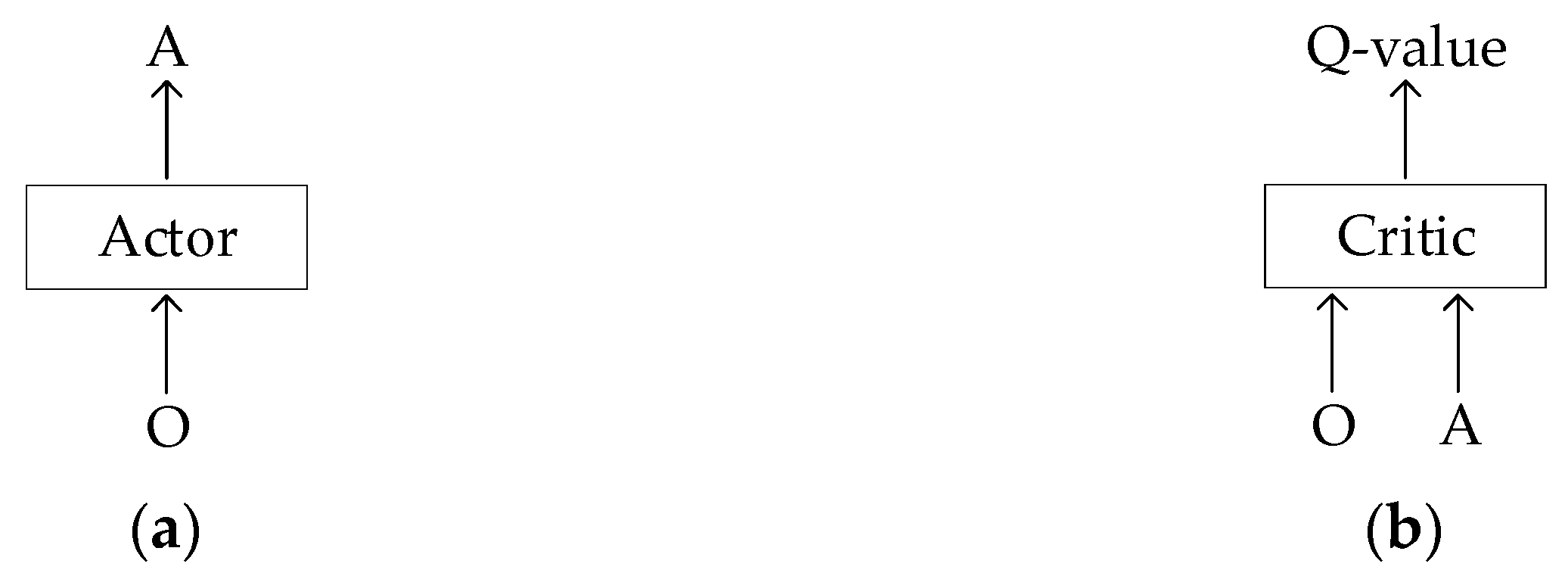
The process of the learning divides machine learning, deep or otherwise, into three subfields: supervised learning, unsupervised learning, and reinforcement learning [25]. In the first two types of learning, only neural networks are considered, which are trained with and without labeled input data, respectively. The third type, reinforcement learning (RL), differs from the first two such that a neural network in RL can be employed as a nonlinear approximator function; this is why the term Deep Reinforcement Learning (deep-RL) is used. The deep-RL can be understood with the concept of an agent, environment, action, observation, and reward, all of which will be discussed in detail. RL is classified into two types: model-based and model-free. The model-based RL has the model of an environment and a planning of agent dynamics, whereas an agent of the model-free RL learns only by values, without explicitly knowing an environment model. Most applications, like this study, are based on model-free RL. In the model-free category, there are three approaches of algorithms for an agent’s learning: value-based, policy-based, and actor-critic. The value-based algorithms are when an agent uses the value function to evaluate the goodness or badness of states. In turn, the policy-based algorithms follow a policy of an agent’s behavior, which is a map from state to action. The actor-critic approach is a mix of value-based and policy-based algorithms; this approach is applied in this paper. Figure 1 shows the summary of machine learning classification from artificial intelligence to RL algorithms.

In this study, the model-free actor-critic RL approach aims to solve the mobile robot exploration problem in indoor environments. There are several algorithms that can be listed under the actor-critic category: Deep Deterministic Policy Gradient (DDPG), Twin Delayed Deep Deterministic Policy Gradients (TD3), Proximal Policy Optimization (PPO), Soft Actor Critic (SAC), and Asynchronous Advantage Actor Critic (A3C). In this study, the off-policy DDPG algorithm is selected for the mapping problem. The DDPG algorithm is useful for robotics applications because it allows the control of electric motors due to continuous output data. The remaining algorithms mentioned above are able to provide continuous actions as well. However, the DDPG learns directly from the observation data, which corresponds to the mapping problem using a laser sensor. In addition, the DDPG algorithm is not often applied to mobile-robot exploration problems, which is a motivation for the authors to study it in practical application.

The contribution of this study is as follows. A custom environment was created especially for exploration using the occupancy map and the robot movement. The environment evaluates the robot’s motion for learning the unknown space using a reward function. In the same way, it denounces the robot for the negative occasions, such as obstacle collisions. Another contribution is the creation of the DDPG agent and training process for the custom environment. At the end of the paper, the positive and negative results of using the DDPG algorithm are presented for the mapping problem. The comparison of the DDPG algorithm and the nature-inspired exploration algorithm shows the advantages and disadvantages of each approach.

It is important to clarify the terminology in this section, as the names for the mobile-robotics and deep-RL fields intersect. The word “environment” is used in both topics, but the meanings are not the same. The environment in mapping means a physical or simulated space with walls and furniture, for example, a room- or an office-like environment. In deep-RL, the environment is the description of the input/output data reactions, model visualization, and reward function. In the proceeding sections, the RL environment will be used to denote this, and the absence of RL means the terms are related to the mobile-robot system.

This paper is structured as follows. Section 2 discusses the related works of the deep-RL algorithms in the mobile-robot field. In Section 3, the theory of deep-RL and DDPG algorithms are explained in detail. In Section 4, the occupancy reward-driven exploration based on the DDPG agent is proposed. The reward parameters and training options are discussed in Section 5. Finally, the simulation results and the comparison are presented in Section 6, which prove the proposed concept in practice.

2. Related Works

With the development of machine learning algorithms, the robotics field obtained novel and alternative resolutions in its domain along with existing classical methods [26]. Although AI and its concept are not a new trend in computer science [27,28], in robotics, a significant number of applications based on machine learning and its deep learning subdomain have been launched recently, with modern AI appearing with the combination of “big data” and neural network architectures [24,29].

In terms of the applications of deep learning in robotic mapping, two major groups of approaches can be highlighted. The first one is deep learning with widely used convolutional neural network (CNN) architecture. It can be said that CNN was inspired by human vision in the manner of how a human is able to perceive objects and use this knowledge for a multitude of tasks. The major function of CNN is to extract features out of images and then to classify them as an object. Thus, it follows that the robot motion based on CNN can be realized in a case when a robot is equipped with a visual sensor that is a camera. An example is the research [30] on mobile-robot exploration using a hierarchical structure that fuses CNN layers with decision-making process. It obtains RGB-D information from the camera as the input and generates the moving direction as the output for the Turtlebot robot. In the same vein, CNN is applied for exploration in another study [31]. In spite of the fact that it is trained on the basis of input images of the floor plans, the output result returns images containing the labels of exit locations in the building. It is assumed that the search of exit locations in the building refers also to the robotic exploration problem and can be called a semantic or visual exploration. More segmentation is processed in another study [32], capturing the labels (books, ceiling, a chair, floor, a table, etc.) from RGB-D video. CNN and dense Simultaneous Localization and Mapping (SLAM) are applied together in order to add the semantic predictions to a map from multiple viewpoints. The human walk trajectories were predicted by CNN in Ref. [33]. The output results help the robot use this information for avoiding obstacles and planning further tasks. Concluding the discussion on the CNN-related approach, it can be emphasized that there are still limitations in training. It is assumed that CNN learns offline, whereas the mobile-robot exploration usually works online. This is why CNN-based mapping is sometimes considered an impractical solution [34].

The second branch of the robot exploration based on deep learning pertains to deep-RL. Neural networks are also employed in this approach with several numbers of layers, hence, the term “deep-RL”. However, NNs are considered function approximators or the so-called policies that can efficiently operate large numbers of actions and states during training. Based on the field of application, a designer can select an appropriate neural network type among built-in RL approximators and well-known approximators, like CNN and RNN.

Table 1. Related works on the mobile-robot exploration using deep-RL.

	RL Algorithm		RL Environment			Map Representation
	Approximator	Agent	Input	Output	Reward
T. Kollar et al. [35]	Support Vector Machine Policy Learning	Policy Search Dynamic Programming	Laser sensor	Discrete action	Squared error reward function	Occupancy map
L. Tai et al. [36]	CNN	Deep Q-network	RGB-D camera	Discrete actions of 3 moving directions	Keep moving is value 1, collision or stop are −50	Corridor environment, Turtlebot, Gazebo
O. Zhelo et al. [37]	Actor-critic network	A3C agent	Laser sensor	Continuous actions	Intrinsic reward	Simulated environment, 3 maps with different floor plans
Z. Lu et al. [41]	Actor-critic network with LTSM module	DDPG agent	Laser sensor, target points	Continuous actions: linear and angular velocities	Novel reward function for avoiding collision	Gazebo
F. Chen et al. [42]	Graph neural networks	Deep Q-network agent	Laser sensor	Sensing action	Raw reward	Occupancy map
H. Li et al. [43]	FCQN with auxiliary task	Deep Q-network agent	Partial map	Discrete action	Heuristic reward function	Occupancy map, ROS
H. Surmann et al. [44]	Actor-critic network	Fast Hybrid CPU/GPU version of A3C agent	Laser sensor, RGB-D camera	Continuous actions: linear and angular velocities	Goal reached is value 20, collision is value of −20	Simulated and real environment, ROS
J. Zhang et al. [45]	Actor-critic network and Neural-SLAM	A3C with generalized advantage estimator	Laser sensor	Discrete action	$-0.04 \mathrm{values} \mathrm{for} \mathrm{each} \mathrm{step},-0.96 \mathrm{for} \mathrm{collision}, \raisebox{1ex}{$1$}\!\left/ \!\raisebox{-1ex}{$3\times 5$}\right.$ for new grid	Occupancy map, Gazebo

presents related works on mobile-robot exploration. The authors analyzed and sorted out the literature based on the main classifications of the RL framework: algorithm, environment, and map representation. In the study of Kollar et al. [35], it can be seen that the support vector machine algorithm, which is related to supervised machine learning, was applied instead of a deep neural network. The exploration is formulated into a model of partially observable Markov decision process (POMDP). The output result in this work is the optimization of the trajectory in the mapping process. In their study [36], Lei Tai et al., proposed to build a map of the corridor environment using depth sensor information. The CNN model extracts the features from the environment, and the value-based Deep Q-network (DQN) executes the obstacle avoidance for the Turtlebot robot. However, its reward strategy does not stimulate the robot to further and faster explore the uncertainties involved. The static values of 1 and −50 can be referred to as the navigation strategy rather than the mapping. The research of Zhelo et al. [37] investigated the reward function known as an intrinsic reward. The robot navigation is trained using targets by the asynchronous advantage actor-critic algorithm (A3C) with external and intrinsic rewards. Apart from the reward, the novel term “mapless navigation” is proposed for the exploration, which is used in other studies, but only for the navigation problem [38,39,40]. Mapless navigation is when the robot drives without any knowledge of the environment (such as obstacle position and the frontier line between explored and unknown areas) to the targets whose positions are visible due to visible light or Wi-Fi signal localization. This kind of navigation for the exploration problem does not have the ability to build any finite map acquisitions.

End-to-end navigation in an unknown environment based on DDPG with long short-term memory (LSTM) is presented in the study of Z. Lu et al. [41]. Its reward function impels the robot to avoid dynamic obstacles and to choose a smooth trajectory. Chen et al. [42] offered the idea to explore uncertainties via exploration graphs in conjunction with graph neural networks and RL. The deep Q-network agent predicts the robot’s optimal sensing action in belief space. The graph abstraction optimizes and generalizes data for the learning process. This combination of the approaches showed efficient mapping results in the comparison with other policy categories of graph neural networks and RL agents. The study of H. Li et al. [43] proposed a new decision approach based on deep-RL. The approach is a Fully Convolution Q-network (FCQN) with an auxiliary task that receives the grid map of the partial environment as input and returns the control policy as output. Shurmann et al. [44] presented and demonstrated real-time exploration using the Turtlebot robot mounted with an RGB-D camera and Hokuyo laser sensor. To conclude the discussion on the deep-RL-related exploration group, Ref. [45], focusing on the search for uncertainties in an occupancy map, can be presented. Refs. [43,45], which use the occupancy-driven reward function, are shown in Table 1. The strategy of keeping the robot moving towards new areas during the process is a key function in mobile-robot exploration. In the same way, the reward function is a significant component in the deep-RL framework. This is the reason for the authors’ interest in the reward strategy applied in the related works and their proposed contribution in this work.

There are many other studies that focus on solving other problems encountered in mobile-robot systems. In particular, deep-RL is frequently applied in navigation [46,47,48,49,50,51,52], path planning [53,54], and collision avoidance [55,56,57,58].

3. Background

This section discusses the theory concept of Reinforcement Learning and its continuous control method—deep deterministic policy gradient (DDPG) [59].

3.1. Reinforcement Learning

Reinforcement Learning (RL) is a goal-oriented approach that extracts successful actions in an area of concern during its training. This method allows a robot to make correct decisions for a task without human intervention. The RL consists of two main parts: an agent and the RL environment (Figure 2).

The process of RL starts with the environment sending its initial observation (or so-called state) to the agent. According to its computation, the agent makes the action in response to this observation. By this, the action changes the environment, which can be good or bad. Then, the environment sends a new observation and a reward for the last action to the agent. It receives and updates its knowledge and then takes the next action based on the computational analysis. The process repeats in this manner until the environment gives the signal of the end of an episode.

The agent can be seen as a computational controller. It contains a policy and a learning algorithm. The policy is a function approximator (deep neural network), which selects appropriate actions with regards to the observations from the RL environment. The learning algorithm component is to search an optimal policy by maximizing the cumulative reward. It continuously updates the policy parameters based on reward, actions, and observations.

In this study, we applied the actor-critic agent belonging to the class of RL algorithms. There are several known varieties of actor-critic agents, which use either a deterministic actor or stochastic actor, with Q-value critic or a value critic. The difference among them is in the manner of how the data of an actor and critic are updated in the process.

3.2. Actor-Critic Deep Deterministic Policy Gradient Algorithm

The DDPG algorithm is a model-free, online, off-policy RL method. The DDPG agent uses a deterministic actor and Q-value critic. The DDPG agent searches for an optimal policy that maximizes the expected cumulative long-term reward. It can be applied only for an RL environment with continuous action spaces [59].

In the DDPG algorithm, the actor-critic architecture applies four function approximations: deterministic actor network, target actor network, critic network, and target critic network. Considering each separately, Figure 3a represents the actor architecture, in which the actor $\mu \left(O, {\theta }^{\mu }\right)$ directly maps the observations $O_i$ to corresponding actions $a_i,$ which maximizes the long-term reward $R$. In Figure 3b, the critic $Q\left(O, A, {\theta }^Q\right)$ takes actions and observations and returns the corresponding expectation $Q$ of long-term reward. The parameters ${\theta }^{\mu }$ and ${\theta }^Q$ are network weights. The general actor-critic architecture is represented in Figure 3c, in which the RL environment passes the observation to the actor and critic. The actor determines the action and sends it to the critic. That is, the critic estimates the value of how much reward the agent will obtain from this situation. Combining the value with the reward $R$ gives the estimated value of receiving the current observation and making the current action.

The actor target network ${\mu }^{\prime }\left(O, {\theta }^{{\mu }^{\prime }}\right)$ and critic target network $Q^{\prime }\left(O, A, {\theta }^{Q^{\prime }}\right)$ are time−delayed copies of their original networks that slowly track the actor and critic networks. The main role of the target networks is to improve the stability in the learning by periodically saving the actor and critic parameters. The weight parameters ${\theta }^{{\mu }^{\prime }}$ and ${\theta }^{Q^{\prime }}$ of the actor and critic target networks are updated by the equations below for $\tau \ll 1$:

$${\theta }^{Q^{\prime }} \leftarrow \tau {\theta }^Q+\left(1-\tau \right){\theta }^{Q^{\prime }}$$

(1)

$${\theta }^{{\mu }^{\prime }} \leftarrow \tau {\theta }^{\mu }+\left(1-\tau \right){\theta }^{{\mu }^{\prime }}$$

(2)

The critic side of the DDPG algorithm updates the critic by minimizing the loss between target $y$ and the original $Q$ value of the critic network through the following equation:

$$L=\frac{1}{M} {\displaystyle \sum }_i{\left(y_i-Q\left(O_i, a_i,{\theta }^Q\right)\right)}^2$$

(3)

The target $y$ is calculated using the Bellman equation:

$$y_i=r_i+\gamma Q^{\prime }\left(O_{i+1}, {\mu }^{\prime }\left(O_{i+1},{\theta }^{{\mu }^{\prime }}\right),{\theta }^{Q^{\prime }}\right)$$

(4)

where $Q^{\prime }$ is the next $Q$ value obtained from target networks, $\gamma$ is the discount factor, and $r$ is the reward at time $i$.

The actor side of the DDPG algorithm updates the actor parameters using the sampled policy gradient using the following equation:

$${\nabla }_{{\theta }^{\mu }} J \approx \frac{1}{M}{\displaystyle \sum }_i{\nabla }_{a}Q\left(O_i, A, {\theta }^Q\right){|}_{A=\mu \left(O_i, {\theta }^{\mu }\right)}·{\nabla }_{{\theta }^{\mu }}\mu \left(O_i,{\theta }^{\mu }\right)$$

(5)

Here, ${\nabla }_{a}Q\left(O_i, A, {\theta }^Q\right)$ is the gradient of the critic output with respect to the action computed by the actor network. The gradient of the actor output is ${\nabla }_{{\theta }^{\mu }}\mu \left(O_i,{\theta }^{\mu }\right)$ with respect to the actor parameters [60].

In the discussion of the DDPG algorithm, which incorporates DQN [61], two trick techniques with data, the replay buffer and the minibatch, cannot be excluded. The replay buffer is like a data stack with ‘last in—first out’ principal operation. The experience tuples $\left(O_i, a_i, r_i,O_{i+1}\right)$ from the RL environment are added to the end of the buffer so that the oldest experience is pushed out. The replay buffer can have a large size, and the large size should be set. The large collection of experiences allows the data not to fall into convergence and divergence issues. The minibatch is a randomly sampled experience taking from the replay buffer. In Equations (3) and (5), the notation $M$ is the minibatch size or the number of sampled experiences. In each time step, the Q-value and policy of critic and actor networks are updated by sampling a minibatch using the batch normalization technique.

For the continuous action spaces of the DDGP algorithm, the exploration is done by adding noise to the current policy using the following equation:

$$a_i=\mu \left(O_t|{\theta }^{\mu }\right)+N_i$$

(6)

where $N_i$ is stochastic noise.

4. The Proposed Occupancy-Reward-Driven Exploration

This section presents the mobile-robot exploration approach using the model-free deep-RL technique, which is DDPG. In the beginning, the issues of the mapping process are discussed. Then, the model of Markov Decision Process (MDP) for the robotic exploration system is presented. The actions, states, and rewards as elements of MDP were introduced in Section 3 in the discussion of the RL framework and DDPG algorithm. Here, we present the MDP model specially designed for the mobile-robot mapping process while noting that the MDP is a model that allows the description of the RL environment only.

Afterwards, the section introduces the main components of the custom RL environment, with its occupancy reward function created for the mobile-robot exploration. Then, the agent of the actor-critic networks is demonstrated at the end of this section.

4.1. The Robotic Exploration Problem Formalization

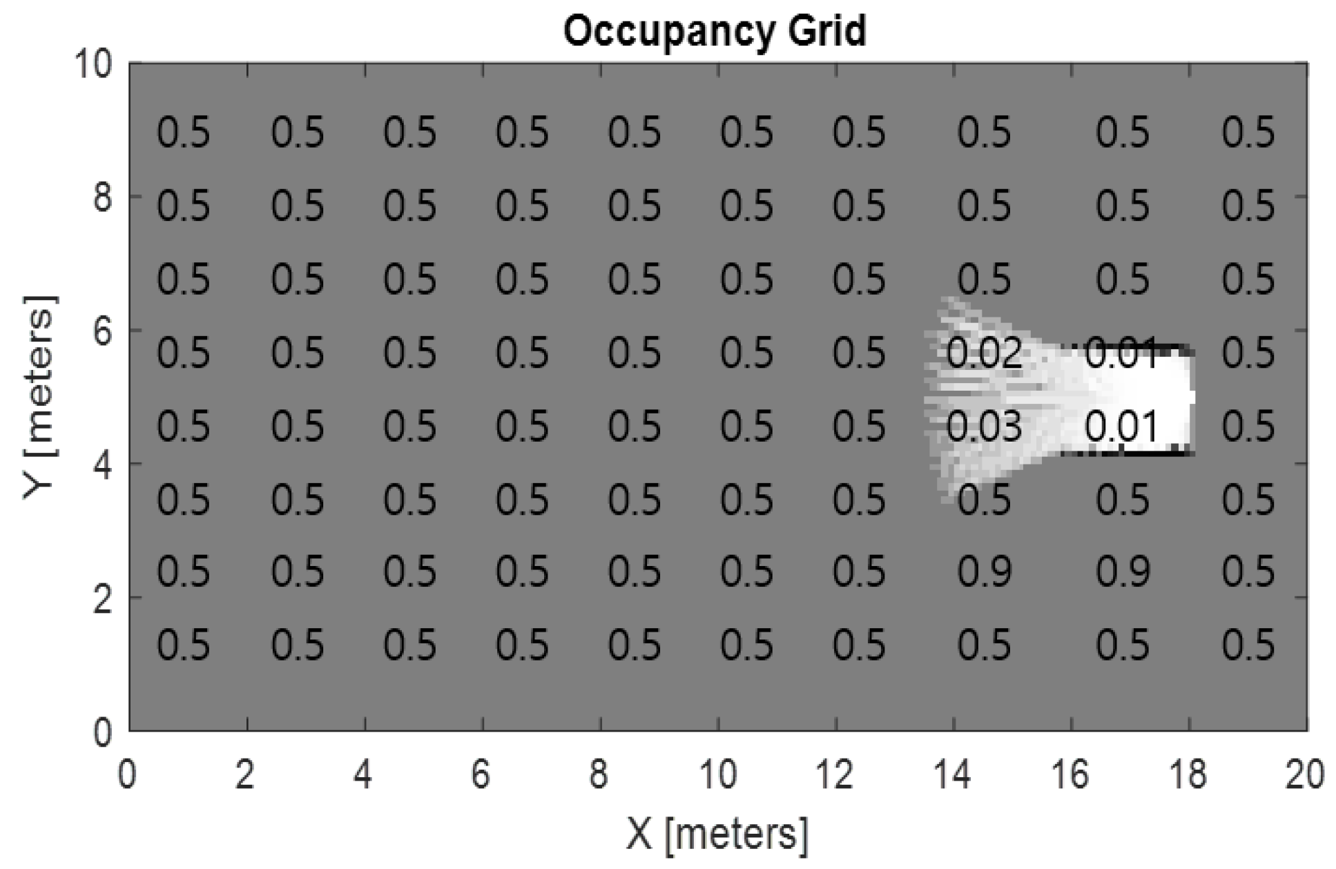
Robotic mapping is a process where a real environment is converted into a digital model by a robot or a group of robots. If we decompose this process into entities, we assume that we obtain two main objects: a robot and an occupancy map. The robot object has a sensor, a position, and velocity parameters. The occupancy map object is massive, with a certain number of cells and their probabilistic values being modified at each time step (Figure 4). The robot begins to run from the initial position. Operating the simulation, this position can be any x-, y-coordinates of the free space on the map. In the real-world experiment, the initial position has zero values on the map, no matter where the robot is currently in a room [21].

As the robot moves in the environment, the occupancy map is updated from every robot position, expanding the terrain acquisition. Step by step, the laser sensor touches new areas or seen areas, which return different probabilities values from the occupancy map. The values from the occupancy map at time $t$ are known as explored segments in this study.

With the aim of continuous and safe driving, some others aspects should be analyzed and planned for the correct sequential decisions. One of these is obstacle avoidance. The decision of turning left or right can be made based on the available visibility for the robot as detected by the laser sensor. The maximum sensing range is a known parameter, depending on the sensor model. Based on the maximum range value, the minimum threshold for the reaction to an obstacle can be defined through test runs. The other parameters for continuous driving are the linear and angular velocities. Their values govern and characterize the robot’s behavior. The linear velocity is responsible for forward and backward motions. When the robot turns, the angular velocity deals with the turning motions.

These metrics, such as the explored segments at each time step, the minimum distance threshold for the obstacle avoidance, and the linear velocity and angular velocity, are synchronized and adjusted in the reward function below.

4.2. MDP Model for the Robotic Exploration

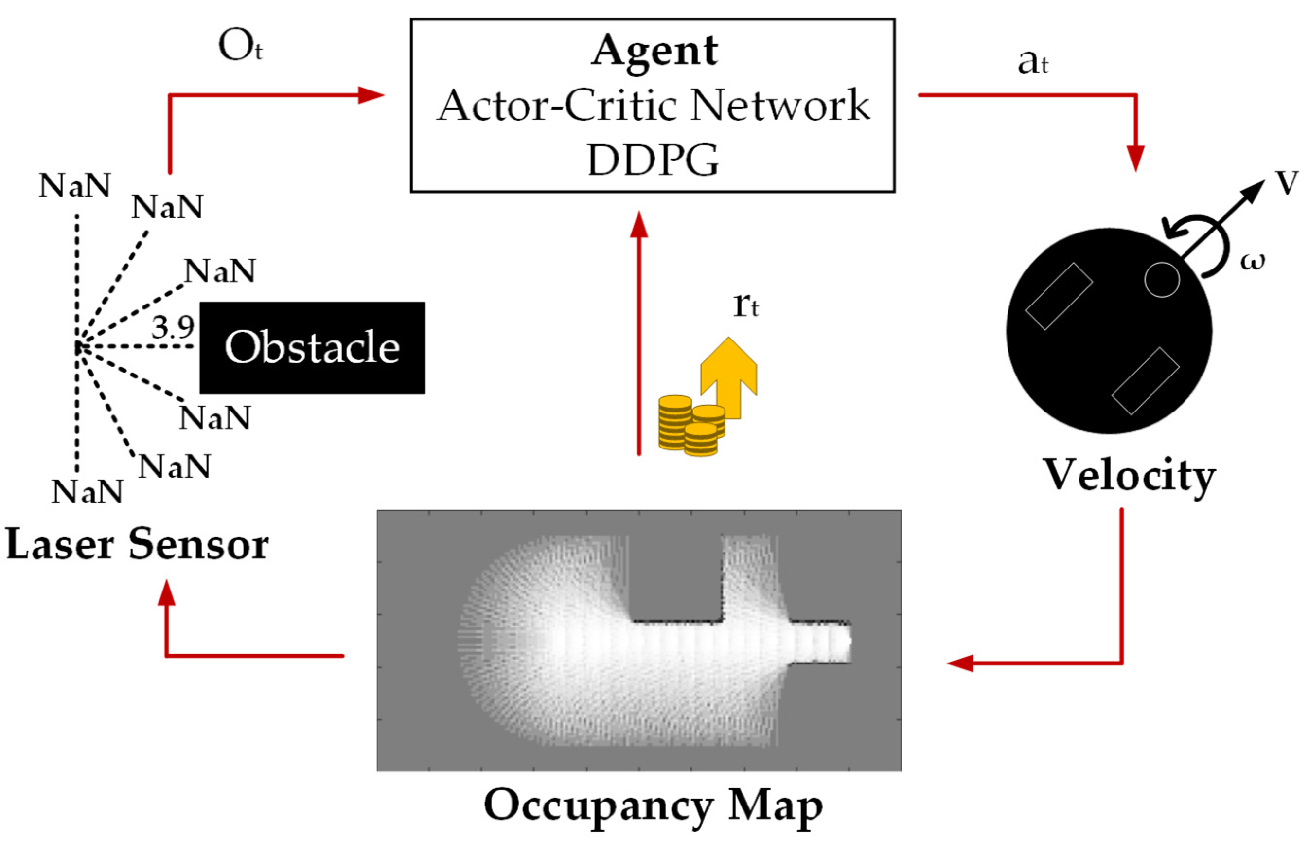
In this paper, the MDP model for robot exploration is formalized as follows. At each iteration $t$, the laser sensor emits and inserts the rays on the occupancy map. If the rays return any numeric data, it means that they hit an obstacle that is located nearby. Otherwise, data of NaN format (Not a Number) denote the absence of obstacles and the presence of free space. Both these types of data are the observations, $O_t$, that are sent to the DDPG agent from the RL environment. For the sake of clarity, the occupancy map is a form of visualization in the RL environment. Furthermore, the function approximator inside of the agent generates and passes actions $a_t$, which are the robot velocities. The RL environment receives the actions, upgrades the occupancy map, and computes a scalar reward $r_t$ according to the changes. Figure 5 illustrates the MDP model based on the robot exploration process.

The reward is a key parameter that motivates the system in making the appropriate decisions. This means that the reward has a strong effect on the motion of the robot. In this paper, the reward is computed according to the explored segments of the occupancy map in each time step $t$. Since the reward is calculated on the RL environment side, the RL environment for the mobile-robot exploration is presented first below. Then, the reward function is introduced in detail in Section 4.4.

4.3. Reinforcement Learning Environment of the Mobile-Robot Exploration

The proposed RL environment, which is presented in Algorithm 1, has a class structure with property values and several certain functions [62]. It is presented in Algorithm 1. The constructor function is the main one, in which the action and observation specifications are defined with their maximum and minimum value ranges. The reset function is called every time the exploration is launched and when the episode is finished during training. In our custom RL environment, in lines 8–15, the reset function sets the map visualization to the initial uncertainties, sets the robot’s initial position, resets the observation values, and activates the ROS interface for the laser scan data and velocity commands.

Algorithm 1: The RL environment for the mobile-robot exploration
1:	classdef ExplorationRLEnv
2:	properties maxRange = 4.095
3:	methods
4:	function constructor
5:	define observation O with lower and upper limit values
6:	define action a with lower and upper limit values
7:	end
8:	function reset
9:	initialize robotPose, observation
10:	map = occupancyMap
11:	enableROSInterface
12:	isDone = false
13:	isBumpedObs = false
14:	reward = 0;
15:	end
16:	function [observation, reward, isDone] = step (constructor, action)
17:	scanMsg = receive(scanSub)
18:	scan = lidarScan(scanMsg)
19:	observation = scan.Ranges
20:	insertRay(map, robotPose, scan, maxRange)
21:	velMsg.Linear.X = action(1)
22:	velMsg.Angular.Z = action(2)
23:	send (velPub, velMsg)
24:	if the last 3 robotPose values are the same
25:	isBumpedObs = true
26:	end
27:	if isMapExplored = true || isBumpedObs = true
28:	isDone = true
29:	resetSimulation
30:	clear(‘node’)
31:	else
32:	isDone = false
33:	end
34:	if t is equal 1
35:	exp = totalMapValues
36:	else
37:	exp = previousReward–totalMapValues
38:	previousReward = totalMapValues
39:	end
40:	reward at time t
41:	end
42:	end
43:	end

Another required function for the RL environment is the step function. The whole process of an episode is carried out in the step function. The action as the input parameter of the step function is taken from the actor-critic neural network of the DDPG agent at each iteration and passed to the robot as the commands of the linear and angular velocities by the ROS publisher node (lines 21–23). The observation as the output parameter receives the sensing laser ranges from the sensor and inserts the rays into the occupancy map in lines 17–20.

Lines 24–26 show the robot’s collision with obstacles in the mapping. The logic of these lines is such that if the values of the robot position are not changed in the last three iterations, the robot has hit an obstacle and cannot avoid it. In essence, the robot does not try to avoid the obstacle as usually occurs using classical algorithms. It only detects the collisions as a bad event that should not be repeated in the next episodes. As the simulation results will show in the next section, this straightforward logic satisfies and can operate correctly for the mobile-robot motion. If the experiment runs in real-world conditions, then a bumper sensor can be used on the robot to detect the collision with an obstacle.

In lines 27–33, the $isDone$ as the output parameter is applied, which is a flag of the episode states. When the flag has true value, the current episode must be finished, and the exploration process should be aborted. This happens in two cases: a map is fully explored or the robot hits an obstacle.

The reward function of lines 34–40 is discussed next in detail.

4.4. Occupancy-Reward-Driven Exploration

The occupancy reward is a function that encourages the robot to seek in unexplored areas to collect knowledge about the indoor environment. The information is gathered from the map with occupancy probability values. In this study, the reward is computed based on the occupancy map $M\left(n,m\right)$ of size $n\times m$. For each time step of an episode, the sum of all map values is summed up and stored in $M$ variable using the following equation:

$$M_t={\displaystyle \sum }_{i=0, j=0}^{n, m}m\left(i,j\right)$$

(7)

In order to observe the amount of explored segment discovered in each time step, the $M$ of the current time must be deducted from those of the previous time:

$$E_t=M_t-M_{t-1}$$

(8)

The function approximator with the reward that is computed only by the explored segments can satisfy the continuous robot driving. However, it was seen during the training process that the robot trajectory is not optimal and not power-efficient. The robot spins constantly.

In view of this undesirable motion, the reward function is proposed as follows:

$$r_t=k\times v_t+q\times w_t^2+d\times s+f\times E_t$$

(9)

where $v_t$ and $w_t$ are linear and angular velocities at time $t$ received from the actor-critic network. The variable $s$ denotes the range of the sensor rays. When the sensor does not meet with the obstacle, the reward obtains the most significant value; in contrast, when the obstacle comes near, the $s$ decreases the reward function. $k$, $q$, $f$, and $d$ are coefficients for the normalization of the reward range.

The reward function should have a range or threshold that can vary. Thus, the actor-critic network during the training process should distinguish between reward values for providing appropriate actions in the RL environment. As equation 9 shows, $r_t$ consists of four factors: linear velocity, angular velocity, sensing ranges, and quantity of the explored segment discovered in one time step. Each has its own priority of how much this factor affects the reward function. The order of priorities in the reward function will be presented in the next section.

Finally, all the rewards are summed as $G$ at the end of the episode after a predefined competing number of time steps, as shown in Equation (10):

$$G=r_t+r_{t+1}+\dots +r_{t+1}$$

(10)

Speaking about the reward, it is necessary to consider the penalty as well. In lines 24–26 of Algorithm 1, the code catches the occasion of obstacle collision. When this happens, the current episode should stop, and the neural network should learn about the unfavorable event. In this case, the reward is assigned a negative number as punishment.

4.5. Deep Deterministic Policy Gradient Agent for the Mobile-Robot Exploration

The RL environment has been constructed. Next, the DDPG agent is presented for the mobile-robot exploration task in Algorithm 2. In general, it can be seen that the agent consists of two main parts: actor-critic network and training.

In lines 1–3, the information about input and output parameters is obtained. These parameters allow the agent to communicate with the RL environment, receiving data and sending computed data.

Algorithm 2: The DDPG agent for the mobile-robot exploration environment
1:	env = ExplorationRLEnv
2:	action = env.getActionInfo
3:	observation = env.getObservationInfo
4:	critic = rlQValueFunction(criticNetwork, observation, action, criticOpts)
5:	actor = rlContinuousDeterministicActor(actorNetwork, observation, action, actorOpts)
6:	agent = rlDDPGAgent(actor, critic, agentOpts)
7:	trainStats = train(agent, env, trainOpts)

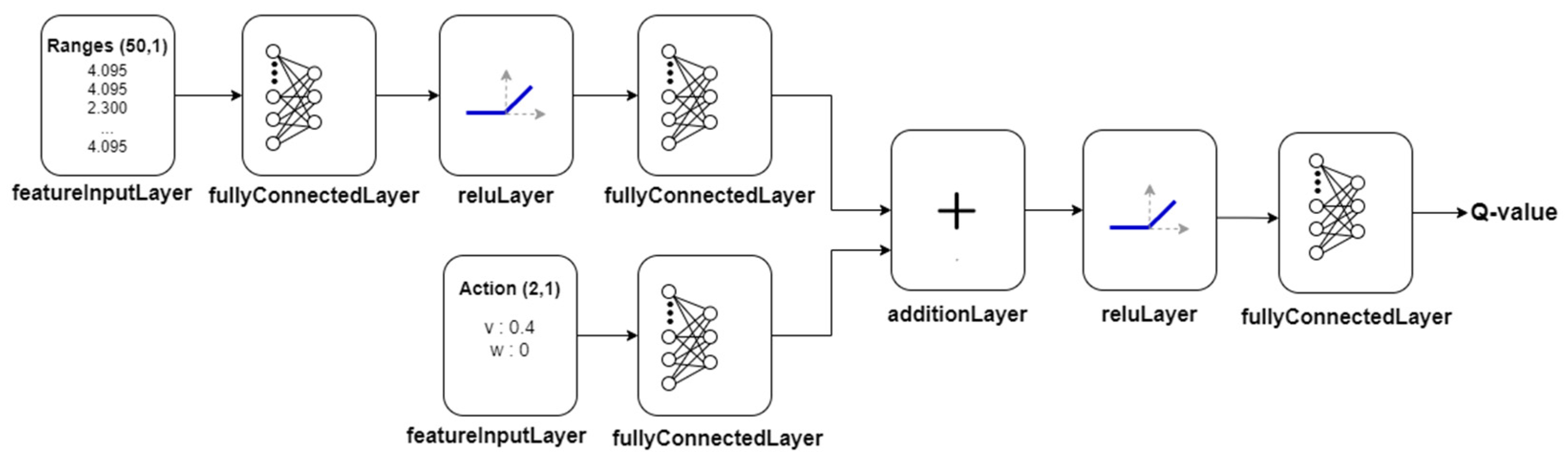
In line 4, the Q-value critic is created using the MATLAB (R2021b release) built-in function, $rlQValueFunction$. Inside the function, four parameters are listed. The main one is a critic network. The remaining ones are the input and output parameters, and setting options of the critic network. Figure 6 shows the architecture of the critic network. It can be seen that the critic network has two paths that later merge into one. The first path starts from the observation data formed in the feature input layer. The observation path contains the fully connected and the relu layers. The second path begins from the action data with 2-D inputs and also contains the fully connected layer. These two paths merge into the addition layer. The output of the critic network is a Q-value, which is a single neuron.

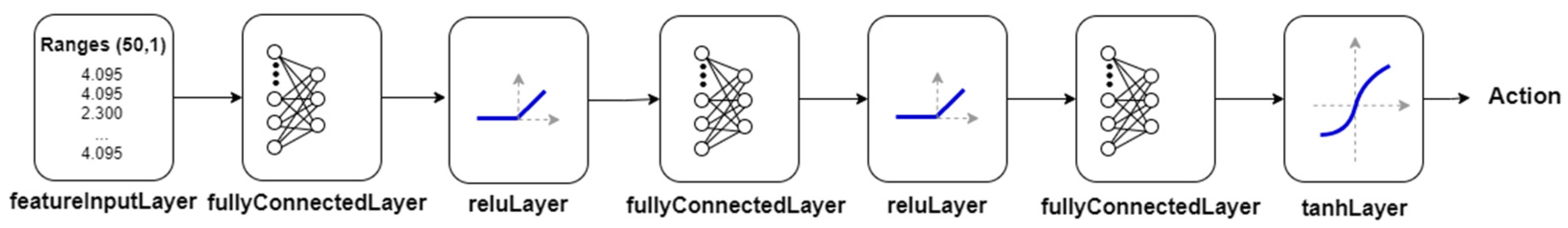
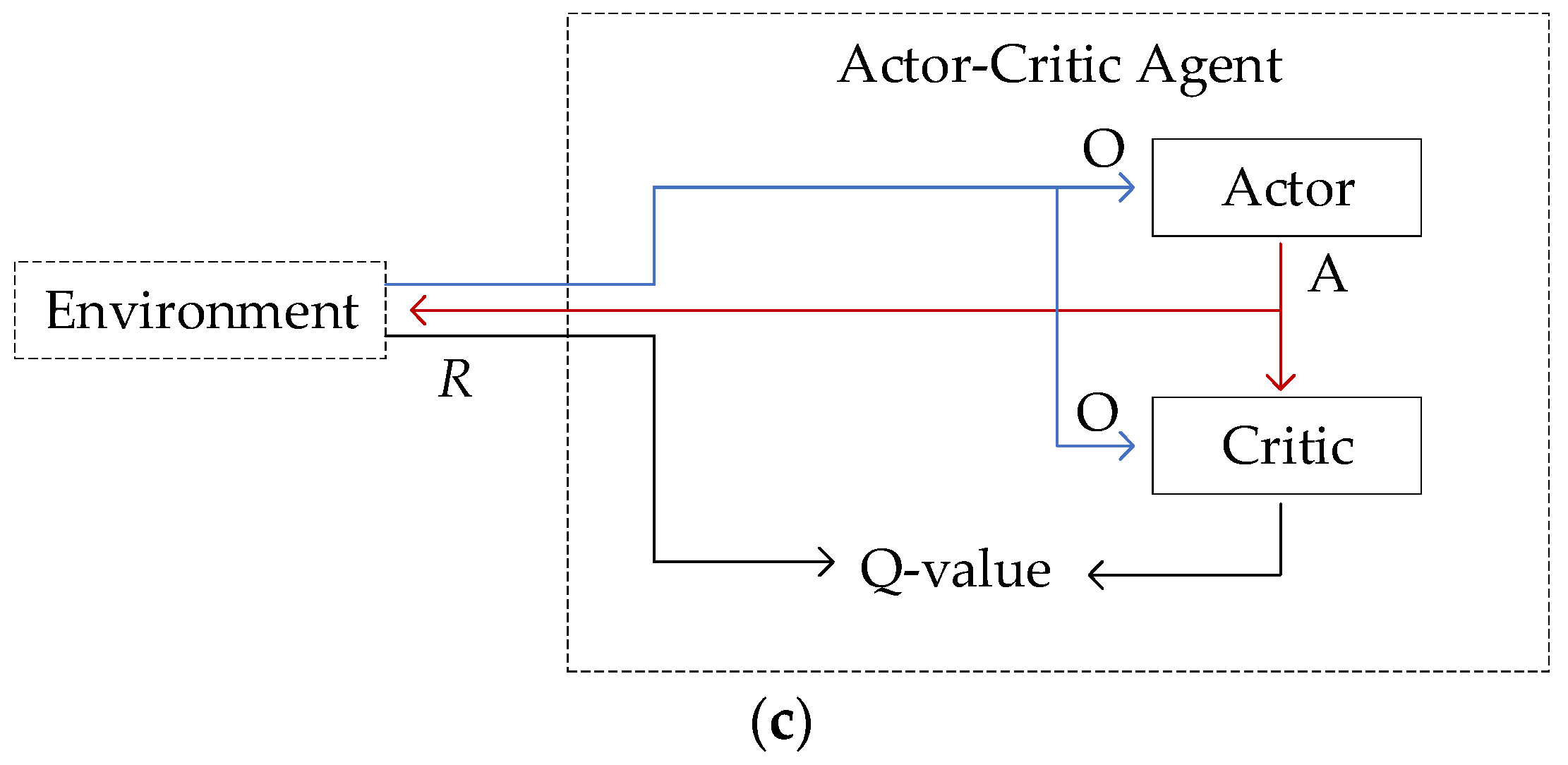
Next, the deterministic actor is created in line 5 using the built-in function, $rlContiniousDeterministicActor$. The actor network is presented in Figure 7. It has one sequence of layers, and it provides direct mapping from the observation to continuous action within tanh scaling. It should be noted that the actor transmits the output data to the critic as illustrated in Figure 3c in Section 3.

Furthermore, in line 6, the DDPG agent is composed, applying the critic and actor in the $rlDDPGAgent$ function. It is important to note here that the setting options, such as $agentOpts$, affect the agent learning. They can be tuned according to the results. In Section 5, values of the setting options are presented for the exploration simulation.

In line 7, the training is launched using the agent and the RL environment. The results are discussed in Section 5.

5. Reward Estimation and Training Options

In this section, the reward function is discussed. The limits and parameter priorities are presented in values. Then, in Section 5.2, the training options of the DDPG agent are performed with their values as well.

5.1. The Reward Estimation

In Section 4.4, we proposed the reward function $r_t$ in Equation (9) for the mobile-robot exploration. The value limit or range for the reward function, which is important to set when using the deep-RL technique, was also discussed. The point is that the RL agent defines the good and bad actions according to the reward function. If the value fluctuates in a chaotic way, then the actor-critic network cannot determine the positive and negative decisions. This is the main reason the value limits for the reward function are defined. When estimating the value, know the upper and lower limits for the parameters in the reward function must be known, which are the linear velocity, the angular velocity, the sensing range distance, and the explored segment.

In

Table 2. The value limits for the reward parameters.

	$\mathit{O}$	$\mathit{v}$	$\mathit{w}$	$\mathit{E}$
Upper limit	${\left[4.095\dots 4.095\right]}^{\prime }$	$0.4$	$0.4$	$239$
Lower limit	${\left[0\dots 0\right]}^{\prime }$	$0$	$-0.4$	$0$

, the value limits for the reward parameters are presented. It can be seen that the upper limit for the observation is $4.095$, which is the maximum sensor range in the simulation. The lower limit is zero. The continuous actions are linear $v$ and angular $w$ velocities, with $0.4$ as upper limits and $0$ and $-0.4$ as lower limits, respectively. The maximum explored segment $E$ is 239, which the sensor of the robot can occupy in the probability occupancy map at time $t$ visiting completely new and free areas. The parameters are normalized in the upper and lower thresholds of the reward function, $-0.2$ and 0.8, respectively.

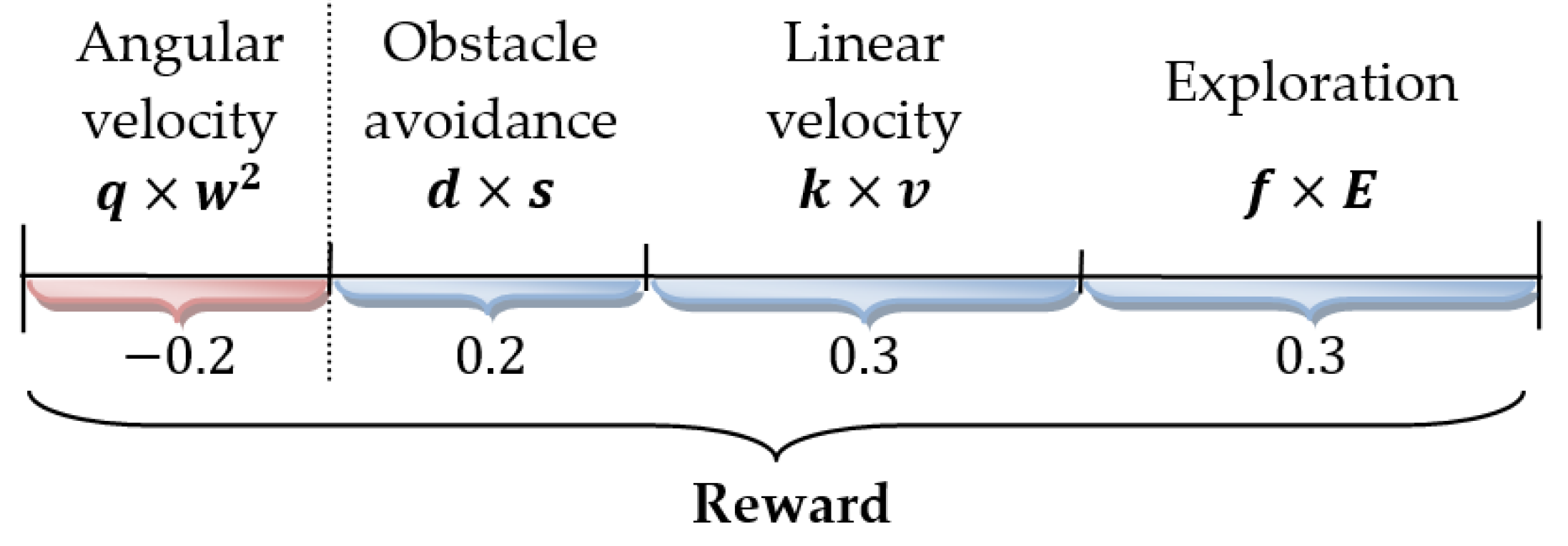
To adjust the parameters, the coefficients $k$, $q$, $d$, $f$ are introduced in Equation (9). However, the priorities of the four parameters in the reward function are included in the coefficient as well, which affects the robot motion in the exploration process. Thus, the priorities can be described as follows: 30% for linear velocity, −20% for angular velocity, 20% for sensing ranges, and 30% for the explored segment. Converting the percentage to numbers, the coefficients are as follows: $k=0.75$, $q=-1.25$, $d=0.07$, and $f=0.0013$. In real-world applications, the proposed coefficients can be used without changes when the robot is Turtlebot2 and the laser sensor is Hokuyo (model no. urg-04lx-ug01). For other cases, the values of the coefficients should be calculated individually according to robot kinematics and sensor specifications.

Figure 8 illustrates the above discussion on parameters affecting the reward function to a greater and lesser extent and the adjustment in their values in one common range. The lower and upper limits are −0.2 and 0.8, respectively.

It is appropriate to clarify the reason why angular velocity ($w$) has a negative value in the reward function. When the robot drives straight in an obstacle-free area, $w$ equals $0$. Driving straight is the most optimal motion according to the mapping and the power energy cost. This is why any other values of the angular velocity, $w<0$ for turning to the right side and $w>0$ to the left side, are negative for the reward function.

5.2. Training Agent

The training is the process of learning and storing the experience for the actor-critic agent. The training options affect the DDPG agent. Consequently, it changes the RL environment.

In Algorithm 2, the DDPG agent for the mobile-robot exploration is presented. In this section, $criticOpts$, $actorOpts$, $agentOpts$, and $trainOpts$ options are given in more detail.

Table 3. The options for the actor and critic.

Critic and Actor Options
Learn rate	${10}^3$
L2 Regularization factor	${10}^4$
Gradient threshold	$1$
Use device	gpu

shows the training option values of the actor-critic neural network. The learning rate option is used to specify the training time needed to reach the optimal result. The $L_2$ regularization factor is used to avoid the overfitting of the training. To speed up the training, GPU can be activated by the “use device” option. We used the local GPU device embedded in the PC, the GeForce GTX 1050 Ti model (compute capability 6.1).

The agent and training options are presented in

Table 4. The options for the agent and training.

Agent Option		Training Option
Sample time	$0.1$	Max episodes	500
Experience buffer length	${10}^6$	Max steps per episode	$150$
Discount Factor	$0.995$	Score averaging window length	$50$
Mini batch size	$100$	Stop training criteria	average reward
Target Smooth Factor	$0.001$	Stop training value	$100$
Agent noise options	${10}^{-5}$	Verbose	true
		Plots	training process

. The sample time option is the time interval of output data returned from the simulation. During training, the DDPG agent stores the simulation data using the experience buffer. In turn, the mini-batch selects the data from the buffer randomly and upgrades the actor and critic. The agent noise option is the stochastic noise model that is added at each time step to the agent.

In the training option, the simulation parameters were selected. The simulation runs five hundred times (max episodes). The training can finish under one of these two conditions: (1) 500 episodes have been completed or (2) the average total rewards have reached one hundred values for the last 50 simulations.

In MATLAB, it is worth noting that the simulation results can be saved as a file, which can be loaded again to continue the training process using $save$ and $load$ commands.

6. Simulation Results and Comparison

In practice, the deep-RL method is about two program files that interact with each other. One of them is the RL environment with reward function and map visualization; another consists of the DDPG agent with the actor-critic network and training option settings. They communicate jointly by input data, output data, and reward.

In this section, the simulation results are presented. The comparison with other algorithms is demonstrated at the end of the section.

6.1. Simulation Results

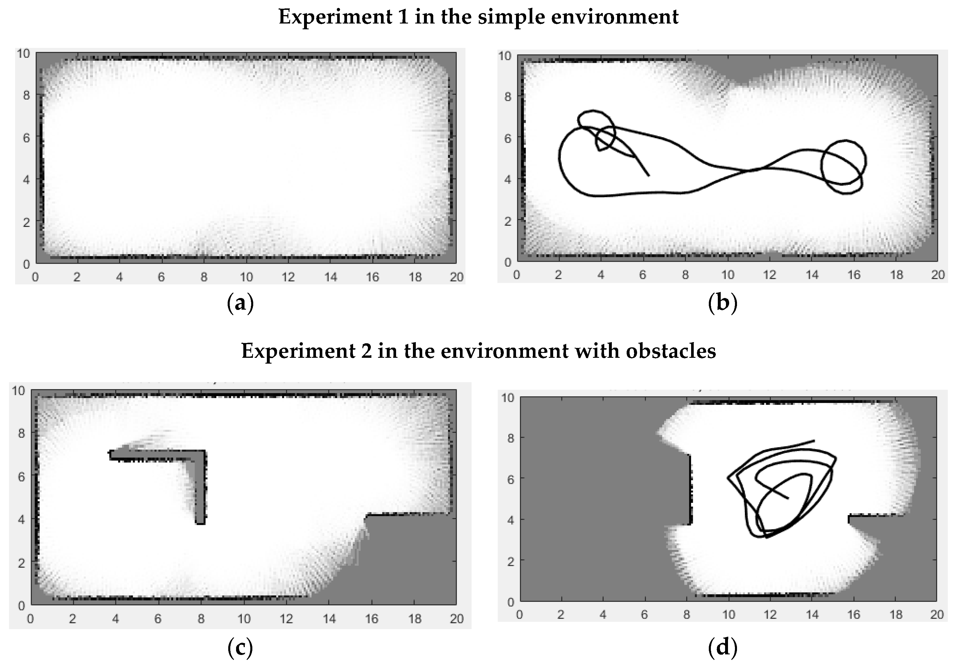
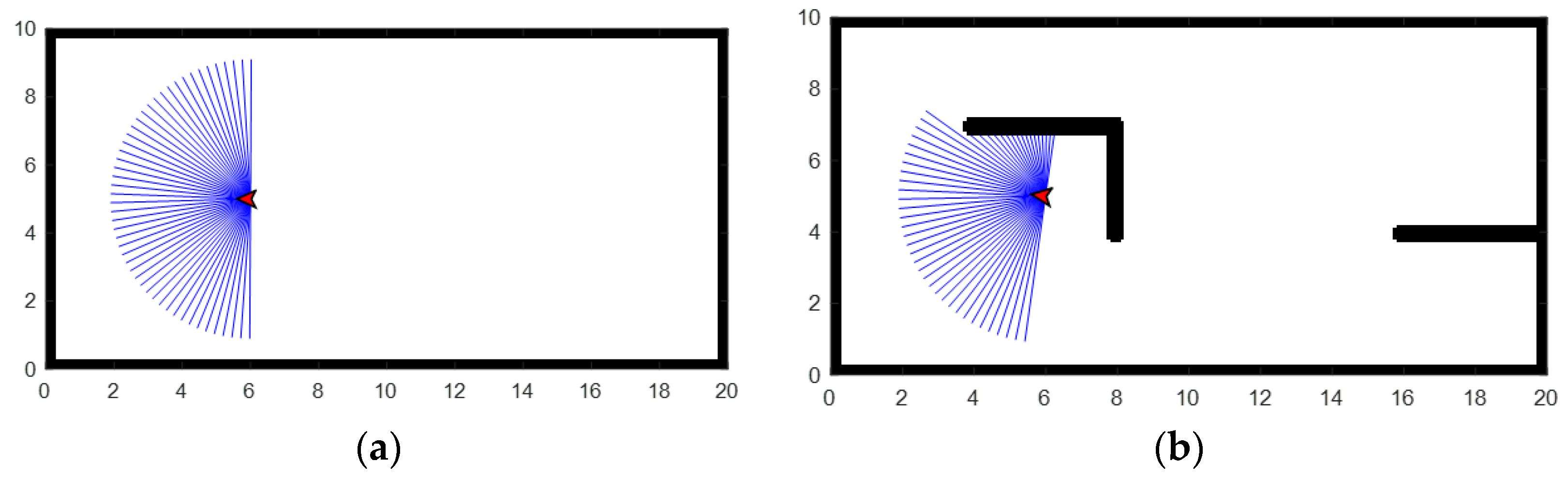
The training DDPG agent and the exploration are carried out online. It means that the robot drives in one episode until time runs out, up 150 steps. Figure 9 shows the environments in which the robot tries to build the maps for two experiments. The first environment is a simple one without obstacles inside the room. The environment of Figure 9b is a more sophisticated version of the first one with obstacles. During the training, the robot drives in one of the environments of Figure 9. Step by step, as it moves during the mapping, it upgrades the occupancy map of Figure 10. It should be noted that the location coordinates of walls and obstacles are not used in the computation. The environments in Figure 9 can be treated as the simulated rooms, which can be easily substituted by real-world environments.

Figure 10 demonstrates the exploration results of training the DDPG agent. Two results from each experiment are presented in (a) map coverage percentage and (b) total reward value. The results were captured during the training according to the greatest values.

Here, it is important to explain the reason for presenting two map results for one experiment. The results of map (a) and map (b) are different because creating a reward function based on only one goal, mapping, does not return a positive result. Several robot behaviors were found to be inappropriate, such as collisions with obstacles, being stuck in one place without any motion, and turning to one side episode after episode. These occurred because the linear velocity, angular velocity, and sensing ranges should be considered in the reward function as they are in the proposed occupancy reward function. This is why the greatest result of the map coverage is not equal to the greatest result of the reward function.

Nonetheless, a full map coverage was obtained. This proves that the DDPG agent is able to provide 99% of the exploration in the simple map (Figure 10a). The greatest reward value ($G=90$) returns a positive result of the exploration in Figure 10b.

In Experiment 2, the training of the DDPG agent was carried out in the environment with obstacles (Figure 10c,d). Two results with the greatest values were taken for the map coverage and reward function categories. It can be seen that the results are worse compared to the results of Experiment 1. Only 86% of the map was explored. The reward function value is 67, which is less than 90.

Based on our practice with the DDPG agent in the mobile-robot exploration, several conclusions can be drawn:

• The agent can solve the mapping problem, especially in a simple environment.
• The reward function can be described as the single objective function. The navigation and exploration of new areas using the reward function of DDPG agent are insufficient for the exploration.
• The mapping performance deteriorates when the number of obstacles in the environment is increased.
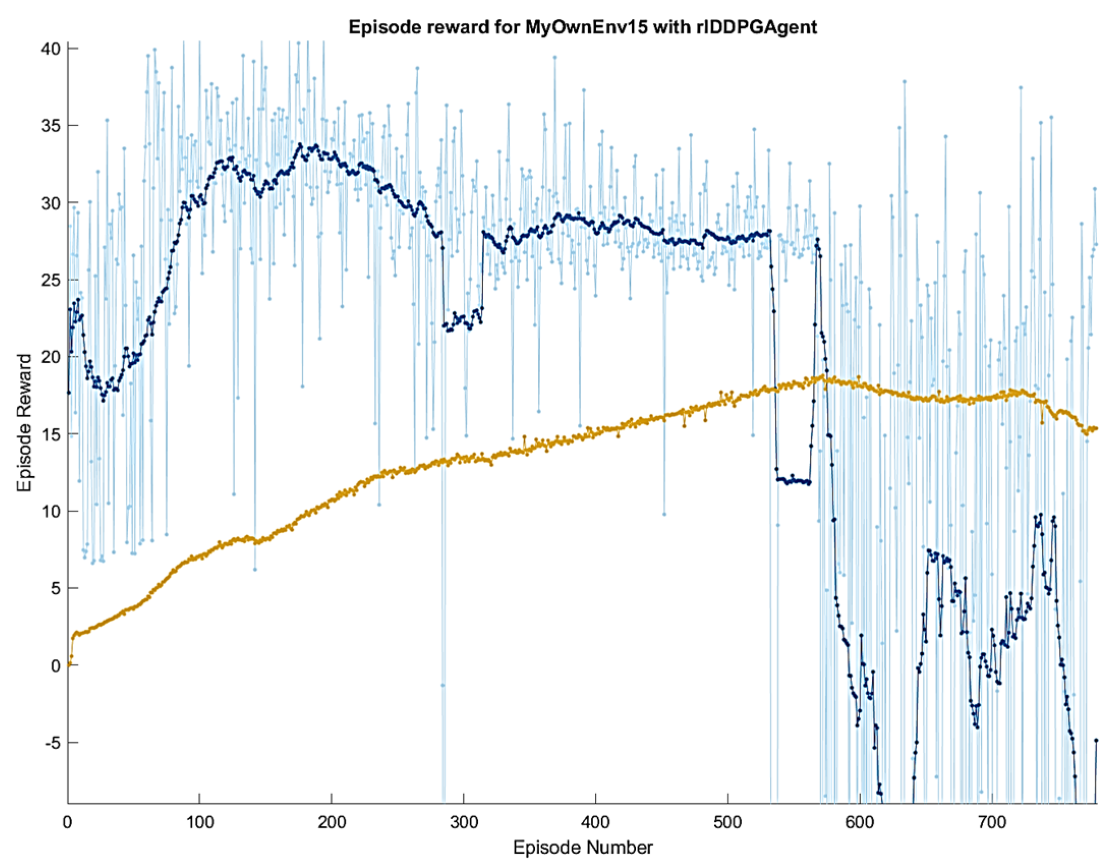
• Increasing the training time did not improve the mapping results. As Figure 11 shows, the overfitting of the neural network occurs in the training after 500 episodes.
• The mapping is a real-time procedure, and the training of the DDPG agent works online as well. The two together used as one system can be considered a time-consuming process.

The experimental results of the proposed occupancy reward-driven exploration using the DDPG agent are recorded and demonstrated in video [63].

6.2. Comparison

In this subsection, the deep-RL and the nature-inspired algorithms are compared. In the authors’ previous studies [21], the GWO algorithm for mobile-robot exploration showed the best result compared with the other nature-inspired optimization techniques. As a consequence, the GWO exploration algorithm is selected for the comparison analysis.

Table 5. Comparison analysis of the GWO exploration and the DDPG agent exploration. The advantages are highlighted in bold.

	Robot Motion	Development	Processing Result	Map Coverage
GWO exploration	Waypoints	Waypoint computation, algorithm logic	Waiting for the best result	91.21%, average result of 10 simulation runs
DDPG exploration	Continuous actions	Two files of RL environment and RL agent	Long training of the agent	99% for simple environment, 86% for complex environment

presents the comparison between the proposed occupancy reward-driven exploration and the nature-inspired exploration. The GWO exploration algorithm works with waypoints. To enable the robot to move somewhere, it needs to provide the robot a point to go to and check that the robot reaches the point in each time step. The continuous action is a more nature-driven action for the robot.

Considering the development criteria, the GWO exploration algorithm requires more work in implementation than the DDPG one. A waypoint should be calculated based on some known parameters (frontier points, robot position) and algorithm logic, which should be considered in the programming. In this case, the DDPG agent is the more intelligent and straightforward developing tool. It should describe the RL environment and denote a reward function. The training process and a neural network find appropriate decisions for the RL environment.

The processing result criteria is about obtaining the best performance of the algorithm. The GWO exploration is a stochastic algorithm that returns different results every simulation run. The best result is unpredictable. It can appear in the first 10 simulation runs or 100 runs. It needs to test and wait for the best result using the GWO exploration algorithm. For the DDPG exploration, the training takes a long time, for instance, 57 h (around 3 days) for the one-experiment result presented in Figure 10.

Considering the map coverage criteria, the DDPG exploration has the greatest percentage result. However, it is only for the free-obstacle environment. Thus, the two approaches are not universal algorithms for the mapping problem. This is a disadvantage.

6.3. Developing Tools

In this study, the DDPG agent was implemented in the MATLAB platform. Several libraries were involved in the exploration simulation: Reinforcement Learning Toolbox, ROS Toolbox, GPU Coder Toolbox, Robotics System Toolbox, Parallel Computing Toolbox, Navigation Toolbox, and Mapping Toolbox.

The exploration with the single robot in the binary occupancy environment and the occupancy map was implemented using $ExampleHelperRobotSimulator$ class.

7. Conclusions

In this paper, the Deep Deterministic Policy Gradient algorithm of deep Reinforcement Learning was deployed in the robotic mapping domain. The custom environment with a reward function was created considering the robot motion principles and the occupancy map visualization. The actor-critic neural network received the sensor data and sent the continuous actions for the robot. The actions in the custom environment were evaluated by the proposed occupancy reward function. The training shows that the DDPG agent can solve the mapping problem in the simple free space with wall obstacles. However, its reward strategy does not stimulate the robot enough for it to explore faster and more efficiently. The reward function is only able to evaluate a single parameter, which is a single action.