
Process-Oriented Stream Classification Pipeline: A Literature Review

 , , and
Abstract
:Featured Application
Abstract
1. Introduction
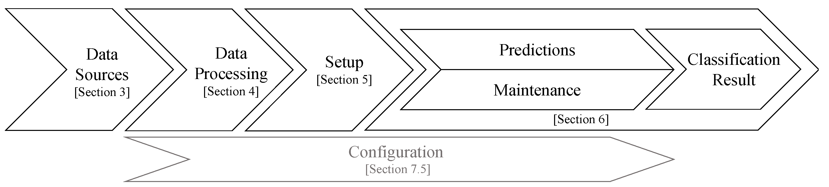
2. Background and Stream Classification Pipeline
2.1. Definition and Requirements of Data Stream Classification
2.2. Process-Oriented Stream Classification Pipeline
2.3. Literature Base
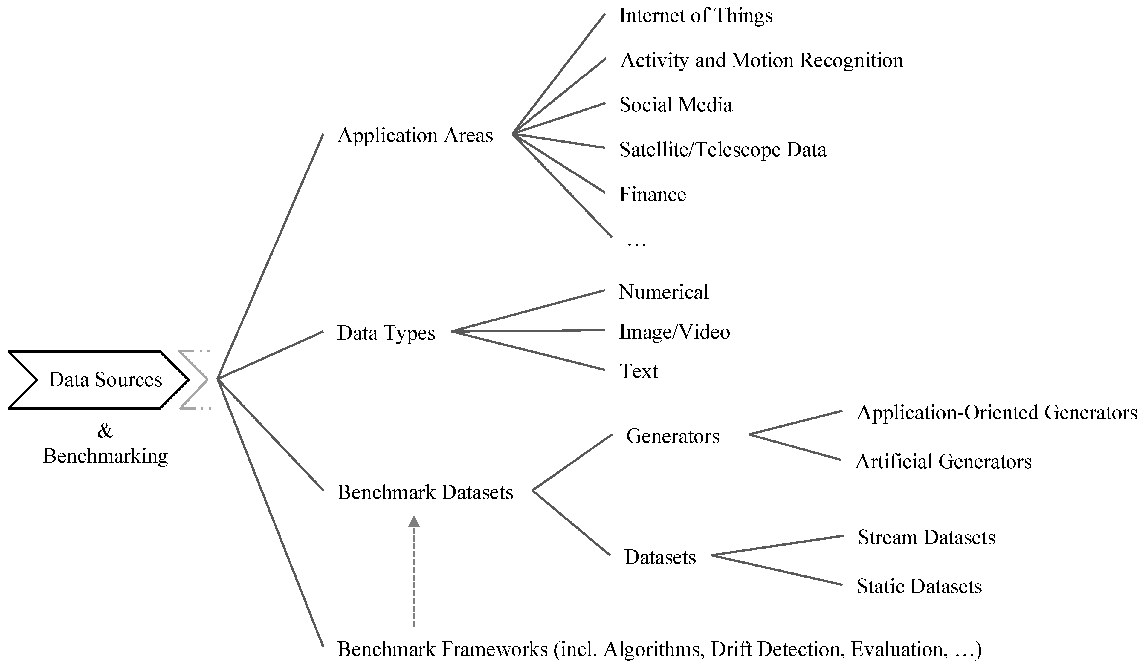
3. Data Sources and Benchmarking
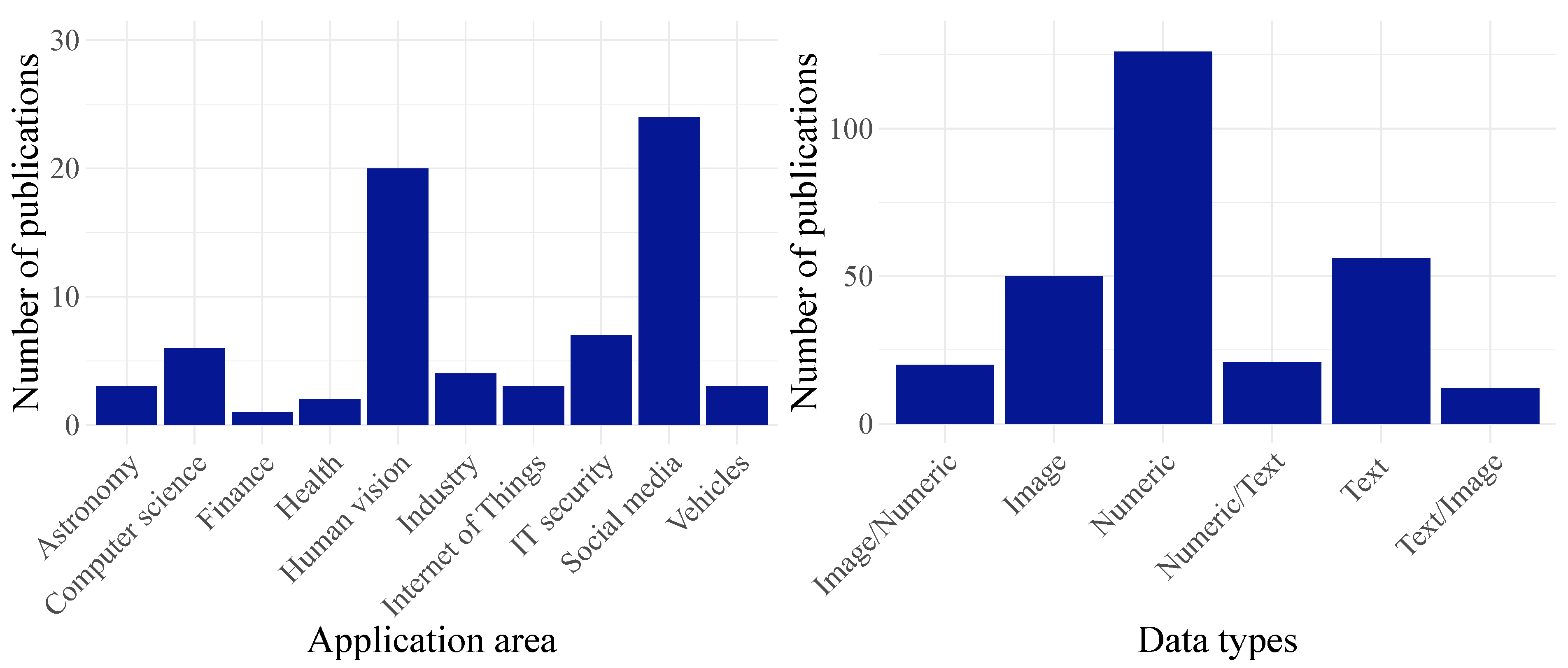
3.1. Application Areas and Data Types
3.2. Benchmark Datasets
3.2.1. Generators

| Generator | Description | Attributes | No. Classes | Concept Drift | |
|---|---|---|---|---|---|
| Artificial | BG-FD [49] | Binary Generator with Feature Drift | 2 categorical | 3 | Feature |
| Circle [47] | Four contexts defined by four circles | 2 numerical | 2 | Gradual | |
| Gauss [47] | Normally distributed data | 2 numerical | 2 | Abrupt | |
| Mixed [47] | Different functions used | 2 numerical, 2 categorical | 2 | Abrupt | |
| RandomRBF [50] | Random Radial Basis Function | Simple: 10 numerical Complex: 50 numerical | Arbitrary | None | |
| R-RBF with drift [50] | Random RBF with drift | Simple: 10 numerical Complex: 50 numerical | Arbitrary | Gradual | |
| RHG [51] | Rotating Hyperplane Generator | Arbitrary | Arbitrary | Gradual, Incremental | |
| RHG with drift [50] | RHG with drift for each attribute | Arbitrary | Arbitrary | Incremental | |
| RTG [51] | Random Tree Generator | Simple: 10 numerical, 10 categorical Complex: 50 numerical, 50 categorical | Arbitrary | Abrupt | |
| RTG-FD [49] | RTG with Feature Drift | Simple: 20/Complex: 100 | 2 | Features | |
| SEA [52] | Streaming Ensemble Algorithm | 3 numerical | 2 | Abrupt | |
| SEA-FD [49] | SEA with Feature Drift | 3 numerical | 2 | Feature | |
| Sine [47] | Points below or above sinus curve | 2 numerical | 2 | Abrupt | |
| STAGGER [53] | Boolean function | 3 categorical | 2 | Abrupt | |
| Application-oriented | Agrawal [54] | Loan applications approval | 6 numerical, 2 categorical | 2 | None |
| LED [55,56] | Digit prediction on LED display | 24 categorical | 2 | Abrupt | |
| LED with drift [50,56] | LED generator with drift | 24 categorical | 2 | Arbitrary | |
| Rotating checkerboard [57] | Generates virtual drift of checkerboard | 2 numerical | 2 | Gradual | |
| WaveForm [48,55] | Detect Wave Form | Simple: 21 numerical Complex: 40 numerical | 3 | Abrupt | |
| WaveForm-FD [48,55] | Detect Wave Form with Feature Drift | Simple: 21 numerical Complex: 40 numerical | 3 | Feature |
| Dataset | Description | Observations | Attributes | No. Classes | Discipline |
|---|---|---|---|---|---|
| Adult [58] | Predict income | 48,842 | 14 mixed types | 2 | Miscellaneous |
| Airline [59] | Flight delays in USA | 116 | 13 mixed types | 2 | Vehicles |
| AWS Prices [60] | Bids on server capacity | 27.5 | 6 mixed types | Arbitrary | Industry |
| CIFAR [61,62] | Tiny colour images | 60,000 | 32 × 32 pixels | 10 | Computer Vision |
| COCO [45] | Text recognition in images | 173,589 | 5 mixed types | Arbitrary | Computer Vision |
| Electricity [47,63] | Relative price changes | 45,312 | 8 mixed types | 2 | Industry |
| ECUE 1 [64] | E-mail spam filtering | 10,983 | 287,034 tokens | 2 | Miscellaneous |
| ECUE 2 [64] | E-mail spam filtering | 11,905 | 166,047 tokens | 2 | Miscellaneous |
| E-Mail data [65] | E-mail headings | 1500 | 913 words | 2 | Social Media |
| Forest Covertype [66] | Covertype for quadrants | 581,012 | 54 mixed types | 7 | Miscellaneous |
| Gas Sensor Array [67,68] | Gas type identification | 13,910 | 8 mixed types | 6 | Industry |
| Kddcup99 [69] | Intrusion detection | 494,021 | 41 mixed types | 23 | IT-Security |
| Keystroke [70] | Detect imposter keystrokes | 20,400 | 31 mixed types | 10 | IT-Security |
| MNIST [71] | Handwritten digits | 70,000 | 28 × 28 pixel | 10 | Computer Vision |
| Luxembourg [72] | Classify internet usage | 1901 | 20 mixed types | 2 | Social Media |
| NOAA Rain [73] | Predict rain | 18,159 | 8 mixed types | 2 | Miscellaneous |
| Nursery [74] | Rank applications for nursery schools | 12,960 | 8 numerc | 5 | Miscellaneous |
| Ozon [75] | Preidct ozone levels | 2534 | 72 mixed types | 2 | Miscellaneous |
| Outdoor objects [76] | Recognize objects in garden | 4000 | 21 mixed types | 40 | Computer Vision |
| Poker Hand [77] | Hand of five cards | 1 | 11 mixed types | 9 | Miscellaneous |
| Powersupply [69] | Predict hour on basis of power supply | 29,928 | 2 numeric | 24 | Industry |
| Rialto Timelaps [78] | Identify buildings | 82,250 | 27 numeric | 10 | Computer Vision |
| Sensor [69] | Identify sensor ID | 2,219,803 | 5 numeric | 54 | Miscellaneous |
| Usenet [79] | Messages sent in groups | 1500 | 99 attributes | 2 | Social Media |
| Spam Assassin Collection [80] | Spam E-Mails | 9324 | 39,917 words | 2 | Social Media |
| Weather [57] | Predict occurrence of rain | 18,159 | 8 mixed types | 2 | Miscellaneous |
3.2.2. Datasets
3.3. Benchmarking Frameworks
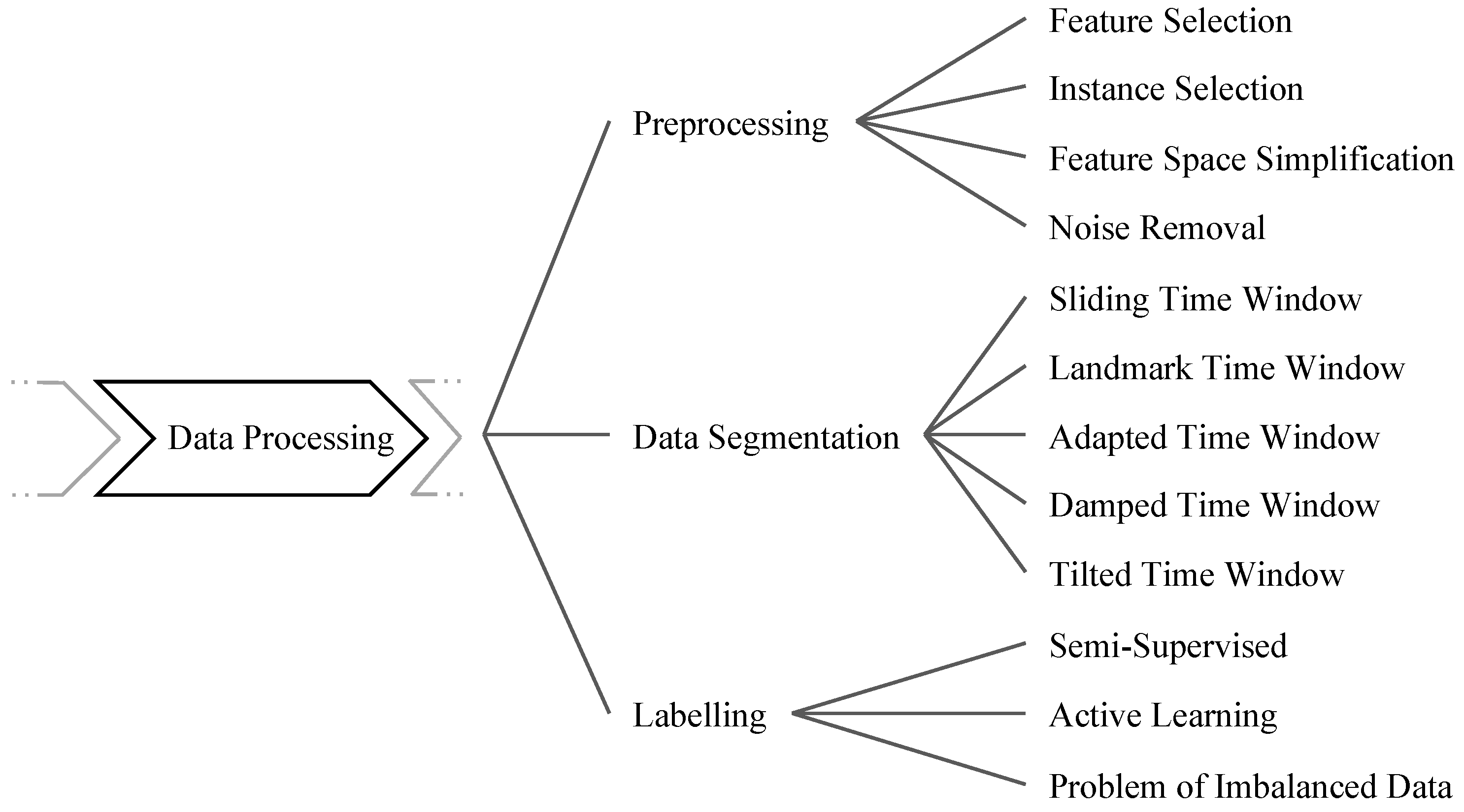
4. Data Processing
4.1. Preprocessing
4.1.1. Feature Selection
4.1.2. Instance Selection
4.1.3. Feature Space Simplification and Noise Removal
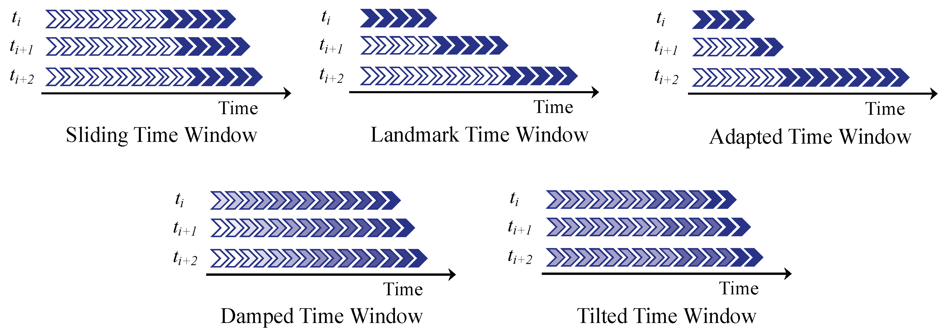
4.2. Data Segmentation
4.3. Labeling
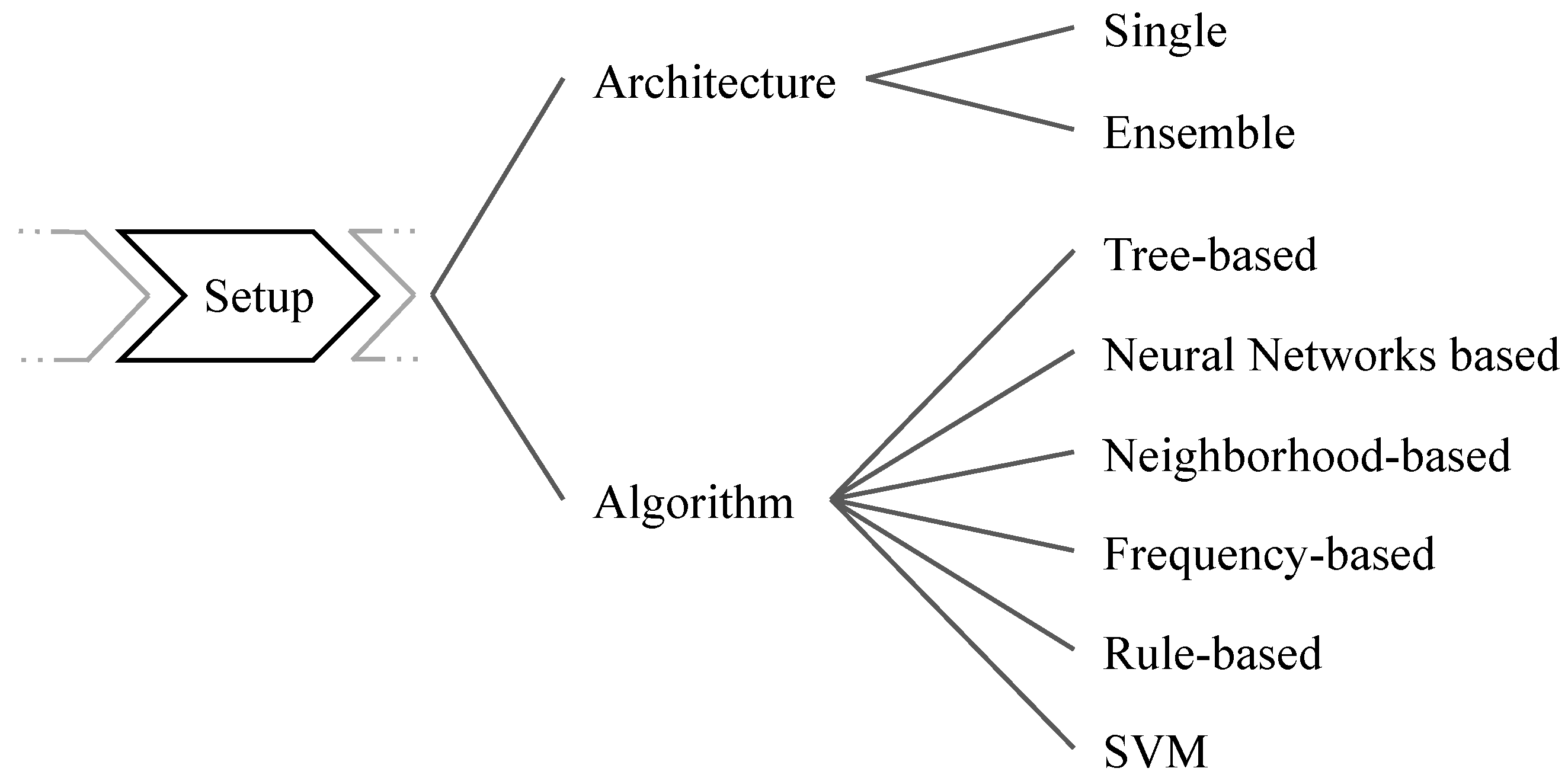
5. Stream Classification Algorithms and Architectures
5.1. Architecture
| Ensemble | Tree | Neural | Neighbor | Rule | Frequency | SVM | Benchmark | |
|---|---|---|---|---|---|---|---|---|
| [120] | ✓ | ✓ | ✓ | ✓ | ||||
| [121] | ✓ | ✓ | ✓ | ✓ | ✓ | ✓ | ||
| [111] | ✓ | ✓ | ✓ | ✓ | ✓ | |||
| [89] | ✓ | ✓ | ✓ | ✓ | ✓ | ✓ | ✓ | |
| [122] | ✓ | ✓ | ✓ | ✓ | ✓ | |||
| [5] | ✓ | |||||||
| [37] | ✓ | ✓ | ✓ | ✓ | ||||
| [1] | ✓ | ✓ | ✓ | ✓ | ||||
| [84] | ✓ | |||||||
| [123] | ✓ | ✓ | ✓ | ✓ | ✓ | |||
| [124] | ✓ | ✓ | ||||||
| [33] | ✓ | ✓ | ✓ | ✓ | ||||
| [125] | ✓ | |||||||
| [13] | ✓ | ✓ | ✓ | ✓ | ✓ | |||
| [88] | ✓ | ✓ | ✓ | ✓ | ✓ | |||
| [7] | ✓ | ✓ | ✓ | ✓ | ||||
| [107] | ✓ | ✓ |
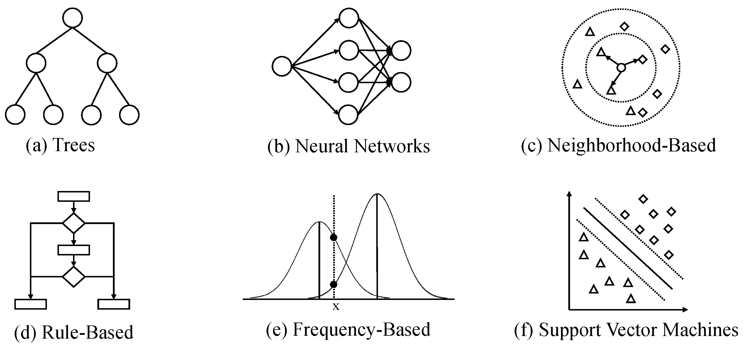
5.2. Algorithms
5.2.1. Trees
5.2.2. Neural Network
5.2.3. Neighborhood Based
5.2.4. Rule-Based
5.2.5. Frequency-Based
5.2.6. Support Vector Machines
5.3. Specific Classification Problems
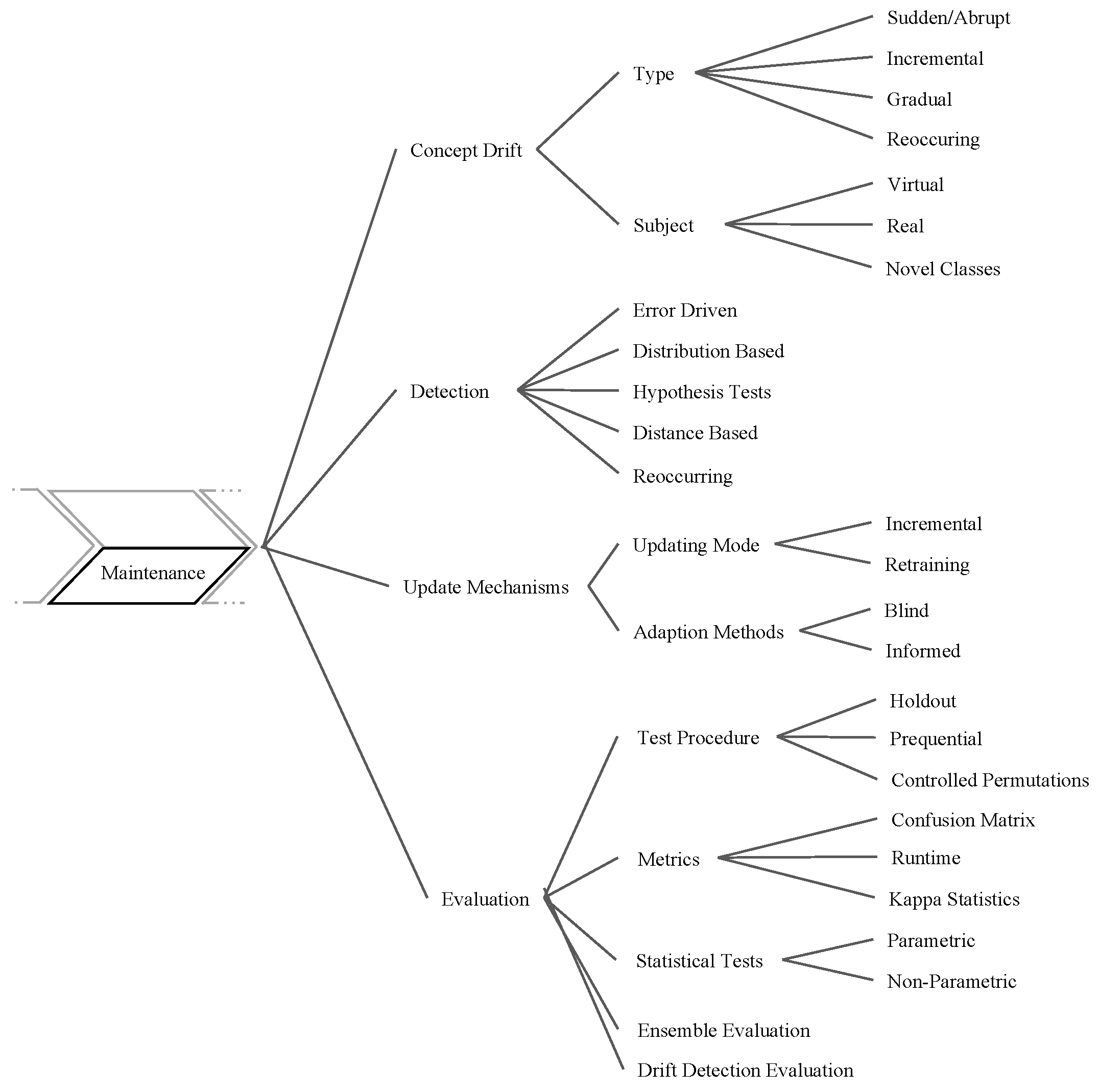
6. Classifier Maintenance
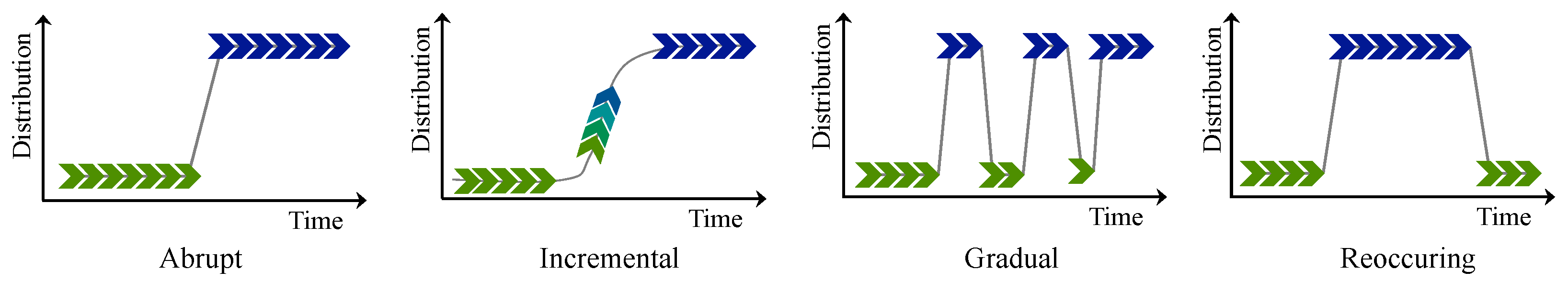
6.1. Concept Drift
6.2. Drift Detection Algorithms
6.2.1. Error Driven
6.2.2. Distribution Based
6.2.3. Statistical Test Based
6.2.4. Semi- and Unsupervised
6.2.5. Reoccurring Concept Detection
6.3. Update Mechanisms
6.3.1. Updating Mode
6.3.2. Adaptation Methods
6.4. Evaluation
6.4.1. Test Procedure
6.4.2. Evaluation Metrics
6.4.3. Statistical Tests
6.4.4. Ensemble Evaluation
6.4.5. Drift Detection Evaluation
7. Current and Future Research Directions
7.1. Central List of Future Research Directions
- The lack of appropriate real-world benchmark datasets is a problem in data stream classification, especially in areas where privacy or other regulations are applied, e.g., in health care or when using social media data. A safe and secure way to share the datasets must be identified and developed.
- Most preprocessing methods (e.g., discretization) still are in preliminary stages, as they have issues with efficiency in stream scenarios.
- Dealing with missing data is a challenging task, especially in evolving data streams.
- The combination of several data stream sources, as well as handling high-dimensional data, is in the early stages.
- Imbalanced data is a problem in data stream classification scenarios. This challenge touches on preprocessing tasks such as under- and oversampling and the actual classification and drift detection methods.
- Neural network-based approaches are often inferior in efficiency.
- A unified metric or concept for evaluation of stream classifiers is still missing. Due to the data’s time dependency and possible verification latencies, current evaluation measures derived from the batch setting are not suitable for stream classification.
- More research regarding the detection of the type of concept drifts is needed.
- Promising potential lies in automated (hyper-)parameter configuration of classification and drift detection algorithms.
7.2. Current Work in the Field
7.2.1. Data Sources and Benchmarking
7.2.2. Data Processing
7.2.3. Stream Classification Algorithms and Architectures
7.2.4. Classifier Maintenance
8. Discussion
Author Contributions
Funding
Institutional Review Board Statement
Informed Consent Statement
Conflicts of Interest
References
- Stefanowski, J.; Brzezinski, D. Stream Classification. In Encyclopedia of Machine Learning and Data Mining; Springer: Boston, MA, USA, 2017; pp. 1191–1199. [Google Scholar] [CrossRef]
- Gracewell, J.J.; Pavalarajan, S. Fall Detection Based on Posture Classification for Smart Home Environment. J. Ambient Intell. Humaniz. Comput. 2019, 12, 3581–3588. [Google Scholar] [CrossRef]
- Zorich, L.; Pichara, K.; Protopapas, P. Streaming Classification of Variable Stars. Mon. Not. R. Astron. Soc. 2020, 492, 2897–2909. [Google Scholar] [CrossRef]
- Gama, J.A.; Žliobait, I.; Bifet, A.; Pechenizkiy, M.; Bouchachia, A. A Survey on Concept Drift Adaptation. ACM Comput. Surv. 2014, 46, 44. [Google Scholar] [CrossRef]
- Gomes, H.M.; Barddal, J.P.; Enembreck, F.; Bifet, A. A Survey on Ensemble Learning for Data Stream Classification. ACM Comput. Surv. (CSUR) 2017, 50, 23. [Google Scholar] [CrossRef]
- Bishop, C.M. Pattern Recognition and Machine Learning; Springer: New York, NY, USA, 2006. [Google Scholar]
- Din, S.U.; Shao, J.; Kumar, J.; Mawuli, C.B.; Mahmud, S.M.H.; Zhang, W.; Yang, Q. Data Stream Classification with Novel Class Detection: A Review, Comparison and Challenges. Knowl. Inf. Syst. 2021, 63, 2231–2276. [Google Scholar] [CrossRef]
- Mohammadi, M.; Al-Fuqaha, A.; Sorour, S.; Guizani, M. Deep Learning for IoT Big Data and Streaming Analytics: A Survey. IEEE Commun. Surv. Tutor. 2018, 20, 2923–2960. [Google Scholar] [CrossRef]
- Al-Osta, M.; Bali, A.; Gherbi, A. Event Driven and Semantic Based Approach for Data Processing on IoT Gateway Devices. J. Ambient Intell. Humaniz. Comput. 2019, 10, 4663–4678. [Google Scholar] [CrossRef]
- Yu, L.; Gao, Y.; Zhang, Y.; Guo, L. A Framework for Classification of Data Stream Application in Vehicular Network Computing. In Proceedings of the Green Energy and Networking, Dalian, China, 4 May 2019; Jin, J., Li, P., Fan, L., Eds.; Springer: Cham, Switzerland, 2019; pp. 57–67. [Google Scholar]
- Grzenda, M.; Kwasiborska, K.; Zaremba, T. Combining Stream Mining and Neural Networks for Short Term Delay Prediction. In Proceedings of the International Joint Conference SOCO’17-CISIS’17-ICEUTE’17, León, Spain, 6–8 September 2017; Springer: Cham, Switzerland, 2017; pp. 188–197. [Google Scholar]
- Wang, Q.; Chen, K. Multi-Label Zero-Shot Human Action Recognition Via Joint Latent Ranking Embedding. Neural Netw. 2020, 122, 1–23. [Google Scholar] [CrossRef]
- Khannouz, M.; Glatard, T. A Benchmark of Data Stream Classification for Human Activity Recognition on Connected Objects. Sensors 2020, 20, 6486. [Google Scholar] [CrossRef]
- Singh, T.; Vishwakarma, D. Video Benchmarks of Human Action Datasets: A Review. Artif. Intell. Rev. 2019, 52, 1107–1154. [Google Scholar] [CrossRef]
- Kumar, E.K.; Kishore, P.; Kumar, M.T.K.; Kumar, D.A. 3D Sign Language Recognition with Joint Distance and Angular Coded Color Topographical Descriptor on a 2–Stream CNN. Neurocomputing 2020, 372, 40–54. [Google Scholar] [CrossRef]
- Anjum, A.; Abdullah, T.; Tariq, M.F.; Baltaci, Y.; Antonopoulos, N. Video Stream Analysis in Clouds: An Object Detection and Classification Framework for High Performance Video Analytics. IEEE Trans. Cloud Comput. 2019, 7, 1152–1167. [Google Scholar] [CrossRef]
- Nahar, V.; Li, X.; Zhang, H.L.; Pang, C. Detecting Cyberbullying in Social Networks using Multi-Agent System. Web Intell. Agent Syst. Int. J. 2014, 12, 375–388. [Google Scholar] [CrossRef]
- Tuarob, S.; Tucker, C.S.; Salathe, M.; Ram, N. An Ensemble Heterogeneous Classification Methodology for Discovering Health-Related Knowledge in Social Media Messages. J. Biomed. Inform. 2014, 49, 255–268. [Google Scholar] [CrossRef]
- Burdisso, S.G.; Errecalde, M.; Montes-y Gómez, M. A Text Classification Framework for Simple and Effective Early Depression Detection over Social Media Streams. Expert Syst. Appl. 2019, 133, 182–197. [Google Scholar] [CrossRef]
- Deviatkin, D.; Shelmanov, A.; Larionov, D. Discovering, Classification, and Localization of Emergency Events via Analyzing of Social Network Text Streams. In Proceedings of the International Conference on Data Analytics and Management in Data Intensive Domains, Moscow, Russia, 9–12 October 2018; Springer: Cham, Switzerland, 2018; pp. 180–196. [Google Scholar]
- Taninpong, P.; Ngamsuriyaroj, S. Tree-Based Text Stream Clustering with Application to Spam Mail Classification. Int. J. Data Min. Model. Manag. 2018, 10, 353–370. [Google Scholar] [CrossRef]
- Hu, X.; Wang, H.; Li, P. Online Biterm Topic Model Based Short Text Stream Classification Using Short Text Expansion and Concept Drifting Detection. Pattern Recognit. Lett. 2018, 116, 187–194. [Google Scholar] [CrossRef]
- Carrasco-Davis, R.; Cabrera-Vives, G.; Förster, F.; Estévez, P.A.; Huijse, P.; Protopapas, P.; Reyes, I.; Martínez-Palomera, J.; Donoso, C. Deep Learning for Image Sequence Classification of Astronomical Events. Publ. Astron. Soc. Pac. 2019, 131, 108006. [Google Scholar] [CrossRef]
- Lyon, R.; Brooke, J.; Knowles, J.; Stappers, B. A Study on Classification in Imbalanced and Partially-Labelled Data Streams. In Proceedings of the 2013 IEEE International Conference on Systems, Man, and Cybernetics, Manchester, UK, 13–16 October 2013; pp. 1506–1511. [Google Scholar]
- Huijse, P.; Estevez, P.A.; Protopapas, P.; Principe, J.C.; Zegers, P. Computational Intelligence Challenges and Applications on Large-Scale Astronomical Time Series Databases. IEEE Comput. Intell. Mag. 2014, 9, 27–39. [Google Scholar] [CrossRef] [Green Version]
- Brandt, M.; Tucker, C.; Kariryaa, A.; Rasmussen, K.; Abel, C.; Small, J.; Chave, J.; Rasmussen, L.; Hiernaux, P.; Diouf, A.; et al. An Unexpectedly Large Count of Trees in the West African Sahara and Sahel. Nature 2020, 587, 78–82. [Google Scholar] [CrossRef]
- Krishnaveni, P.; Sutha, J. Novel Deep Learning Framework for Broadcasting Abnormal Events Obtained From Surveillance Applications. J. Ambient Intell. Humaniz. Comput. 2020, 11, 4123. [Google Scholar] [CrossRef]
- Ali, M.; Ali, R.; Hussain, N. Improved Medical Image Classification Accuracy on Heterogeneous and Imbalanced Data using Multiple Streams Network. Int. J. Adv. Comput. Sci. Appl. 2021, 12, 617–622. [Google Scholar] [CrossRef]
- Ding, Y.; Li, Z.; Yastremsky, D. Real-time Face Mask Detection in Video Data. arXiv 2021, arXiv:2105.01816. [Google Scholar]
- Liu, L.; Lei, W.; Wan, X.; Liu, L.; Luo, Y.; Feng, C. Semi-Supervised Active Learning for COVID-19 Lung Ultrasound Multi-symptom Classification. In Proceedings of the 2020 IEEE 32nd International Conference on Tools with Artificial Intelligence (ICTAI), Baltimore, MD, USA, 9–11 November 2020; pp. 1268–1273. [Google Scholar] [CrossRef]
- Sun, J.; Li, H.; Fujita, H.; Fu, B.; Ai, W. Class-Imbalanced Dynamic Financial Distress Prediction Based on Adaboost-SVM Ensemble Combined with SMOTE and Time Weighting. Inf. Fusion 2020, 54, 128–144. [Google Scholar] [CrossRef]
- Vanschoren, J.; van Rijn, J.N.; Bischl, B.; Torgo, L. OpenML: Networked Science in Machine Learning. SIGKDD Explor. Newsl. 2014, 15, 49–60. [Google Scholar] [CrossRef]
- Srivani, B.; Sandhya, N.; Padmaja Rani, B. Literature review and analysis on big data stream classification techniques. Int. J. Knowl.-Based Intell. Eng. Syst. 2020, 24, 205–215. [Google Scholar] [CrossRef]
- Souza, V.M.A.; dos Reis, D.M.; Maletzke, A.G.; Batista, G.E.A.P.A. Challenges in Benchmarking Stream Learning Algorithms with Real-World Data. Data Min. Knowl. Discov. 2020, 34, 1805–1858. [Google Scholar] [CrossRef]
- Gomes, H.M.; Read, J.; Bifet, A.; Barddal, J.P.; Gama, J.a. Machine Learning for Streaming Data: State of the Art, Challenges, and Opportunities. SIGKDD Explor. Newsl. 2019, 21, 6–22. [Google Scholar] [CrossRef]
- Lu, J.; Liu, A.; Dong, F.; Gu, F.; Gama, J.; Zhang, G. Learning Under Concept Drift: A Review. IEEE Trans. Knowl. Data Eng. 2018, 31, 2346–2363. [Google Scholar] [CrossRef] [Green Version]
- Janardan; Mehta, S. Concept drift in Streaming Data Classification: Algorithms, Platforms and Issues. Procedia Comput. Sci. 2017, 122, 804–811. [Google Scholar] [CrossRef]
- Heywood, M. Evolutionary model building under streaming data for classification tasks: Opportunities and challenges. Genet. Program. Evolvable Mach. 2014, 16, 283–326. [Google Scholar] [CrossRef]
- Bifet, A.; Read, J.; Žliobaitė, I.; Pfahringer, B.; Holmes, G. Pitfalls in Benchmarking Data Stream Classification and How to Avoid Them. Prague, Czech Republic, 23–27 September 2013; Blockeel, H., Kersting, K., Nijssen, S., Železný, F., Eds.; Springer: Berlin/Heidelberg, Germany, 2013; pp. 465–479. [Google Scholar] [CrossRef]
- Zheng, X.; Li, P.; Chu, Z.; Hu, X. A Survey on Multi-Label Data Stream Classification. IEEE Access 2019, 8, 1249–1275. [Google Scholar] [CrossRef]
- Engelen, J.; Hoos, H. A survey on semi-supervised learning. Mach. Learn. 2020, 109, 373–440. [Google Scholar] [CrossRef]
- Narasimhamurthy, A.; Kuncheva, L.I. A Framework for Generating Data to Simulate Changing Environments. In Proceedings of the 25th Conference on IASTED International Multi-Conference: Artificial Intelligence and Applications, Innsbruck, Austria, 12–14 February 2007; ACTA Press: Anaheim, CA, USA, 2007; pp. 384–389. [Google Scholar]
- Zhao, J.; Jing, X.; Yan, Z.; Pedrycz, W. Network traffic classification for data fusion: A survey. Inf. Fusion 2021, 72, 22–47. [Google Scholar] [CrossRef]
- Tidjon, L.N.; Frappier, M.; Mammar, A. Intrusion Detection Systems: A Cross-Domain Overview. IEEE Commun. Surv. Tutor. 2019, 21, 3639–3681. [Google Scholar] [CrossRef]
- Veit, A.; Matera, T.; Neumann, L.; Matas, J.; Belongie, S. COCO-Text: Dataset and Benchmark for Text Detection and Recognition in Natural Images. arXiv 2016, arXiv:cs.CV/1601.07140. [Google Scholar]
- Assenmacher, D.; Weber, D.; Preuss, M.; Calero Valdez, A.; Bradshaw, A.; Ross, B.; Cresci, S.; Trautmann, H.; Neumann, F.; Grimme, C. Benchmarking Crisis in Social Media Analytics: A Solution for the Data Sharing Problem. Soc. Sci. Comput. Rev. (SSCR) J. 2021, 39. [Google Scholar] [CrossRef]
- Gama, J.; Medas, P.; Castillo, G.; Rodrigues, P. Learning with Drift Detection. In Proceedings of the Brazilian Symposium on Artificial Intelligence; Springer: Sao Luis, Maranhao, Brazil, 2004; pp. 286–295. [Google Scholar]
- Aha, D. Waveform Database Generator Data Set. 2021. Available online: http://archive.ics.uci.edu/ml/datasets/waveform+database+generator+%28version+1%29 (accessed on 5 September 2022).
- Barddal, J.P.; Murilo Gomes, H.; Enembreck, F. A Survey on Feature Drift Adaptation. In Proceedings of the 27th International Conference on Tools with Artificial Intelligence, Vietri sul Mare, Italy, 9–11 November 2015; Volume 127, pp. 1053–1060. [Google Scholar] [CrossRef]
- Bifet, A.; Gavaldà, R.; Holmes, G.; Pfahringer, B. Machine Learning for Data Streams: With Practical Examples in MOA; The MIT Press: Cambridge, MA, USA, 2018. [Google Scholar] [CrossRef]
- Hulten, G.; Spencer, L.; Domingos, P. Mining Time-Changing Data Streams. In Proceedings of the Seventh ACM SIGKDD International Conference on Knowledge Discovery and Data Mining, San Francisco, CA, USA, 26–29 August 2001; ACM: New York, NY, USA, 2001; pp. 97–106. [Google Scholar] [CrossRef]
- Street, W.N.; Kim, Y. A Streaming Ensemble Algorithm (SEA) for Large-Scale Classification. In Proceedings of the Seventh ACM SIGKDD International Conference on Knowledge Discovery and Data Mining, San Francisco, CA, USA, 26–29 August 2001; ACM: New York, NY, USA, 2001; pp. 377–382. [Google Scholar] [CrossRef]
- Schlimmer, J.C.; Granger, R.H. Incremental Learning from Noisy Data. Mach. Learn. 1986, 1, 317–354. [Google Scholar] [CrossRef]
- Agrawal, R.; Imielinski, T.; Swami, A. Database Mining: A Performance Perspective. IEEE Trans. Knowl. Data Eng. 1993, 5, 914–925. [Google Scholar] [CrossRef]
- Breiman, L.; Friedman, J.H.; Olshen, R.A.; Stone, C.J. Classification and Regression Trees; Brooks/Cole Publishing: Monterey, CA, USA, 1984. [Google Scholar]
- Aha, D. LED Display Domain Data Set. 2021. Available online: https://archive.ics.uci.edu/ml/datasets/LED+Display+Domain (accessed on 5 September 2022).
- Elwell, R.; Polikar, R. Incremental Learning of Concept Drift in Nonstationary Environments. IEEE Trans. Neural Netw. 2011, 22, 1517–1531. [Google Scholar] [CrossRef]
- Kohavi, R. Scaling up the accuracy of naive-Bayes classifiers: A decision-tree hybrid. In Proceedings of the Second International Conference on Knowledge Discovery and Data Mining, Portland, OR, USA, 2–4 August 1996. [Google Scholar]
- Data Expo. Airline On-Time Performance. 2018. Available online: http://stat-computing.org/dataexpo/2009/ (accessed on 5 September 2022).
- Visser, B.; Gouk, H. AWS Spot Pricing Market. 2018. Available online: https://www.openml.org/d/41424 (accessed on 5 September 2022).
- Krizhevsky, A. Learning Multiple Layers of Features from Tiny Images; Technical Report; University of Toronto: Toronto, ON, Canada, 2009. [Google Scholar]
- Li, H. CIFAR10-DVS: An event-stream dataset for object classification. Front. Neurosci. 2017, 11, 309. [Google Scholar] [CrossRef] [PubMed]
- Harries, M. SPLICE-2 Comparative Evaluation: Electricity Pricing; Technical Report; University of South Wales: South Wales, UK, 1999. [Google Scholar]
- Delany, S.J.; Cunningham, P.; Tsymbal, A.; Coyle, L. A case-based technique for tracking concept drift in spam filtering. Knowl. Based Syst. 2005, 18, 187–195. [Google Scholar] [CrossRef]
- Katakis, I.; Tsoumakas, G.; Vlahavas, I. Tracking Recurring Contexts Using Ensemble Classifiers: An Application to Email Filtering. Knowl. Inf. Syst. 2010, 22, 371–391. [Google Scholar] [CrossRef]
- Blackard, J.; Dean, D. Comparative Accuracies of Artificial Neural Networks and Discriminant Analysis in Predicting Forest Cover Types from Cartographic Variables. Comput. Electron. Agric. 1999, 24, 131–151. [Google Scholar] [CrossRef]
- Vergara, A.; Vembu, S.; Ayhan, T.; Ryan, M.A.; Homer, M.L.; Huerta, R. Chemical gas sensor drift compensation using classifier ensembles. Sens. Actuators B Chem. 2012, 166–167, 320–329. [Google Scholar] [CrossRef]
- Rodriguez-Lujan, I.; Fonollosa, J.; Vergara, A.; Homer, M.; Huerta, R. On the calibration of sensor arrays for pattern recognition using the minimal number of experiments. Chemom. Intell. Lab. Syst. 2014, 130, 123–134. [Google Scholar] [CrossRef]
- Zhu, X. Stream Data Mining Repository. 2010. Available online: https://www.cse.fau.edu/~xqzhu/stream.html (accessed on 5 September 2022).
- Killourhy, K.; Maxion, R. Why Did My Detector Do That?! In Proceedings of the Recent Advances in Intrusion Detection, Ottawa, ON, Canada, 15–17 September 2010; Jha, S., Sommer, R., Kreibich, C., Eds.; Springer: Berlin/Heidelberg, Germany, 2010; pp. 256–276. [Google Scholar]
- Lecun, Y.; Bottou, L.; Bengio, Y.; Haffner, P. Gradient-Based Learning Applied to Document Recognition. Proc. IEEE 1998, 86, 2278–2324. [Google Scholar] [CrossRef]
- Žliobaitė, I. Combining Similarity in Time and Space for Training Set Formation Under Concept Drift. Intell. Data Anal. 2011, 15, 589–611. [Google Scholar] [CrossRef]
- Ditzler, G.; Polikar, R. Incremental Learning of Concept Drift from Streaming Imbalanced Data. IEEE Trans. Knowl. Data Eng. 2013, 25, 2283–2301. [Google Scholar] [CrossRef]
- Zupan, B.; Bohanec, M.; Bratko, I.; Demsar, J. Machine Learning by Function Decomposition. In Proceedings of the Fourteenth International Conference on Machine Learning; Morgan Kaufmann, Nashville, TN, USA, 8–12 July 1997. [Google Scholar]
- Zhang, K.; Fan, W. Forecasting Skewed Biased Stochastic Ozone Days: Analyses, Solutions and Beyond. Knowl. Inf. Syst. 2008, 14, 299–326. [Google Scholar] [CrossRef]
- Losing, V.; Hammer, B.; Wersing, H. Interactive online learning for obstacle classification on a mobile robot. In Proceedings of the International Joint Conference on Neural Networks, Killarney, Ireland, 12–17 July 2015; pp. 1–8. [Google Scholar] [CrossRef]
- Cattral, R.; Oppacher, F.; Deugo, D. Supervised and Unsupervised Data Mining with an Evolutionary Algorithm. Recent Adv. Comput. Comput. Commun. 2002, 2, 296–300. [Google Scholar] [CrossRef]
- Losing, V.; Hammer, B.; Wersing, H. KNN Classifier with Self Adjusting Memory for Heterogeneous Concept Drift. In Proceedings of the 2016 IEEE 16th International Conference on Data Mining (ICDM), Barcelona, Spain, 12–15 December 2016; Volume 1, pp. 291–300. [Google Scholar] [CrossRef]
- Katakis, I.; Tsoumakas, G.; Vlahavas, I. An Ensemble of Classifiers for coping with Recurring Contexts in Data Streams. In Proceedings of the 18th European Conference Artificial Intelligence, European Coordinating Committee for Artificial Intelligence, Patras, Greece, 21 July 2008; pp. 763–764. [Google Scholar] [CrossRef]
- Katakis, I.; Tsoumakas, G.; Vlahavas, I. Dynamic Feature Space and Incremental Feature Selection for the Classification of Textual Data Streams. In Proceedings of the ECML/PKDD-2006 International Workshop on Knowledge Discovery from Data Streams, Berlin, Germany, 18–22 September 2006; Springer: Berlin/Heidelberg, Germany, 2006; p. 107. [Google Scholar]
- He, Y.; Sick, B. CLeaR: An adaptive continual learning framework for regression tasks. AI Perspect 2021, 3, 2. [Google Scholar] [CrossRef]
- Zliobaite, I. How good is the Electricity benchmark for evaluating concept drift adaptation. arXiv 2013, arXiv:cs.LG/1301.3524. [Google Scholar]
- Žliobaitė, I.; Bifet, A.; Read, J.; Pfahringer, B.; Holmes, G. Evaluation Methods and Decision Theory for Classification of Streaming Data with Temporal Dependence. Mach. Learn. 2015, 98, 455–482. [Google Scholar] [CrossRef]
- Krawczyk, B.; Minku, L.L.; Gama, J.; Stefanowski, J.; Woźniak, M. Ensemble learning for data stream analysis: A survey. Inf. Fusion 2017, 37, 132–156. [Google Scholar] [CrossRef]
- Wares, S.; Isaacs, J.; Elyan, E. Data Stream Mining: Methods and Challenges for Handling Concept Drift. SN Appl. Sci. 2019, 1, 1412. [Google Scholar] [CrossRef]
- Wankhade, K.; Dongre, S.; Jondhale, K. Data stream classification: A review. Iran J. Comput. Sci. 2020, 3, 239–260. [Google Scholar] [CrossRef]
- Gartner IT Glossary. Frameworks. 2021. Available online: https://www.gartner.com/en/information-technology/glossary/framework (accessed on 5 September 2022).
- Bahri, M.; Bifet, A.; Gama, J.; Gomes, H.M.; Maniu, S. Data stream analysis: Foundations, major tasks and tools. WIREs Data Min. Knowl. Discov. 2021, 11, e1405. [Google Scholar] [CrossRef]
- Nguyen, H.L.; Woon, Y.K.; Ng, W.K. A Survey on Data Stream Clustering and Classification. Knowl. Inf. Syst. 2015, 45, 535–569. [Google Scholar] [CrossRef]
- Inoubli, W.; Aridhi, S.; Mezni, H.; Maddouri, M.; Nguifo, E. A comparative study on streaming frameworks for big data. In Proceedings of the Very Large Data Bases (VLDB), Rio de Janeiro, Brazil, 27–31 August 2018; Springer: Berlin/Heidelberg, Germany, 2018. [Google Scholar]
- García, S.; Ramírez-Gallego, S.; Luengo, J.; Benítez, J.M.; Herrera, F. Big data preprocessing: Methods and prospects. Big Data Anal. 2016, 1, 9. [Google Scholar] [CrossRef]
- Hulten, G.; Domingos, P. VFML: Very Fast Machine Learning Toolkit for Mining High-Speed Data Streams. 2004. Available online: https://www.cs.washington.edu/dm/vfml/ (accessed on 5 September 2022).
- Jubatus Team. Framework and Library for Distributed Online Machine Learning. 2019. Available online: http://jubat.us/en/ (accessed on 5 September 2022).
- Apache Software Foundation. Apache Spark–Unified Analytics Engine for Big Data. 2021. Available online: https://spark.apache.org (accessed on 5 September 2022).
- Noah’s Ark Lab. streamDM: Data Mining for Spark Streaming. 2016. Available online: http://huawei-noah.github.io/streamDM/ (accessed on 5 September 2022).
- Montiel, J.; Halford, M.; Mastelini, S.M.; Bolmier, G.; Sourty, R.; Vaysse, R.; Zouitine, A.; Gomes, H.M.; Read, J.; Abdessalem, T.; et al. River: Machine Learning for Streaming Data in Python. arXiv 2020, arXiv:cs.LG/2012.04740. [Google Scholar]
- Bifet, A.; Holmes, G.; Pfahringer, B.; Kranen, P.; Kremer, H.; Jansen, T.; Seidl, T. MOA: Massive Online Analysis. A Framework for Stream Classification and Clustering. In Proceedings of the First Workshop on Applications of Pattern Analysis, Windsor, UK, 1–3 September 2010; pp. 44–50. [Google Scholar]
- Hall, M.; Frank, E.; Holmes, G.; Pfahringer, B.; Reutemann, P.; Witten, I.H. The WEKA Data Mining Software: An Update. SIGKDD Explor. Newsl. 2009, 11, 10–18. [Google Scholar] [CrossRef]
- Ramírez-Gallego, S.; Krawczyk, B.; García, S.; Woźniak, M.; Herrera, F. A Survey on Data Preprocessing for Data Stream Mining: Current Status and Future Directions. Neurocomputing 2017, 239, 39–57. [Google Scholar] [CrossRef]
- Masud, M.M.; Chen, Q.; Gao, J.; Khan, L.; Han, J.; Thuraisingham, B. Classification and Novel Class Detection of Data Streams in a Dynamic Feature Space. In Proceedings of the Machine Learning and Knowledge Discovery in Databases, Athens, Greece, 5–9 September 2011; Balcázar, J.L., Bonchi, F., Gionis, A., Sebag, M., Eds.; Springer: Berlin/Heidelberg, Germany, 2010; pp. 337–352. [Google Scholar]
- Beringer, J.; Hüllermeier, E. Efficient Instance-based Learning on Data Streams. Intell. Data Anal. 2007, 11, 627–650. [Google Scholar] [CrossRef] [Green Version]
- Gama, J.A.; Pinto, C. Discretization from Data Streams: Applications to Histograms and Data Mining. In Proceedings of the 2006 ACM Symposium on Applied Computing, Dijon, France, 23–27 April 2006; ACM: New York, NY, USA, 2006; pp. 662–667. [Google Scholar] [CrossRef]
- Prati, R.C.; Luengo, J.; Herrera, F. Emerging topics and challenges of learning from noisy data in nonstandard classification: A survey beyond binary class noise. Knowl. Inf. Syst. 2019, 60, 63–97. [Google Scholar] [CrossRef]
- Sun, B.; Chen, S.; Wang, J.; Chen, H. A Robust Multi-Class AdaBoost Algorithm for Mislabeled Noisy Data. Knowl.-Based Syst. 2016, 102, 87–102. [Google Scholar] [CrossRef]
- Alghushairy, O.; Alsini, R.; Soule, T.; Ma, X. A Review of Local Outlier Factor Algorithms for Outlier Detection in Big Data Streams. Big Data Cogn. Comput. 2020, 5, 1. [Google Scholar] [CrossRef]
- Yala, N.; Fergani, B.; Fleury, A. Towards Improving Feature Extraction and Classification for Activity Recognition on Streaming Data. J. Ambient Intell. Humaniz. Comput. 2017, 8, 177–189. [Google Scholar] [CrossRef]
- Tieppo, E.; Santos, R.R.d.; Barddal, J.P.; Nievola, J.C. Hierarchical classification of data streams: A systematic literature review. Artif. Intell. Rev. 2021, 54, 1–40. [Google Scholar] [CrossRef]
- Zhu, Y.; Shasha, D. StatStream: Statistical Monitoring of Thousands of Data Streams in Real Time. In Proceedings of the 28th International Conference on Very Large Databases; Bernstein, P.A., Ioannidis, Y.E., Ramakrishnan, R., Papadias, D., Eds.; Morgan Kaufmann: San Francisco, CA, USA, 2002; Chapter 32; pp. 358–369. [Google Scholar] [CrossRef]
- Ng, W.; Dash, M. Discovery of Frequent Patterns in Transactional Data Streams. In Transactions on Large-Scale Data- and Knowledge-Centered Systems II; Springer: Berlin/Heidelberg, Germany, 2010; pp. 1–30. [Google Scholar] [CrossRef]
- Bifet, A.; Gavalda, R. Learning from Time-Changing Data with Adaptive Windowing. In Proceedings of the 2007 SIAM International Conference on Data Mining; Society for Industrial and Applied Mathematics (SIAM): Philadelphia, PA, USA, 2007; pp. 443–448. [Google Scholar]
- Aggarwal, C.C. A Survey of Stream Classification Algorithms. In Data Classification: Algorithms and Applications; Charu, C., Aggarwal, V.K., Eds.; CRC Press: New York, NY, USA, 2014; Chapter 9; pp. 245–274. [Google Scholar]
- Khamassi, I.; Sayed Mouchaweh, M.; Hammami, M.; Ghédira, K. Discussion and review on evolving data streams and concept drift adapting. Evol. Syst. 2018, 9, 1–23. [Google Scholar] [CrossRef]
- Masud, M.M.; Woolam, C.; Gao, J.; Khan, L.; Han, J.; Hamlen, K.W.; Oza, N.C. Facing the Reality of Data Stream Classification: Coping with Scarcity of Labeled Data. Knowl. Inf. Syst. 2012, 33, 213–244. [Google Scholar] [CrossRef]
- Žliobaitė, I.; Bifet, A.; Pfahringer, B.; Holmes, G. Active Learning with Drifting Streaming Data. IEEE Trans. Neural Netw. Learn. Syst. 2013, 25, 27–39. [Google Scholar] [CrossRef] [PubMed]
- Arabmakki, E.; Kantardzic, M. SOM-Based Partial Labeling of Imbalanced Data Stream. Neurocomputing 2017, 262, 120–133. [Google Scholar] [CrossRef]
- Chawla, N.V.; Bowyer, K.W.; Hall, L.O.; Kegelmeyer, W.P. SMOTE: Synthetic Minority Over-sampling Technique. J. Artif. Intell. Res. 2002, 16, 321–357. [Google Scholar] [CrossRef]
- Krawczyk, B.; Stefanowski, J.; Wozniak, M. Data Stream Classification and Big Data Analytics. Neurocomputing 2015, 150, 238–239. [Google Scholar] [CrossRef]
- Iwashita, A.S.; Papa, J.P. An Overview on Concept Drift Learning. IEEE Access 2019, 7, 1532–1547. [Google Scholar] [CrossRef]
- Pan, S.; Zhang, Y.; Li, X. Dynamic Classifier Ensemble for Positive Unlabeled Text Stream Classification. Knowl. Inf. Syst. 2012, 33, 267–287. [Google Scholar] [CrossRef]
- Gaber, M.M.; Zaslavsky, A.; Krishnaswamy, S. A Survey of Classification Methods in Data Streams. In Data Streams; Advances in Database Systems; Aggarwal, C.C., Ed.; Springer: Boston, MA, USA, 2007; Volume 31, pp. 39–59. [Google Scholar] [CrossRef]
- Lemaire, V.; Salperwyck, C.; Bondu, A. A Survey on Supervised Classification on Data Streams. Bus. Intell. 2014, 4, 88–125. [Google Scholar]
- Barddal, J.P.; Gomes, H.M.; de Souza Britto, A.; Enembreck, F. A benchmark of classifiers on feature drifting data streams. In Proceedings of the 2016 23rd International Conference on Pattern Recognition (ICPR), Cancun, Mexico, 4–8 December 2016; pp. 2180–2185. [Google Scholar] [CrossRef]
- Losing, V.; Hammer, B.; Wersing, H. Incremental on-line learning: A review and comparison of state of the art algorithms. Neurocomputing 2018, 275, 1261–1274. [Google Scholar] [CrossRef]
- Nagendran, N.; Sultana, H.P.; Sarkar, A. A Comparative Analysis on Ensemble Classifiers for Concept Drifting Data Streams. In Soft Computing and Medical Bioinformatics; SpringerBriefs in Applied Sciences and Technology; Springer: Singapore, 2019; pp. 55–62. [Google Scholar] [CrossRef]
- Li, L.; Sun, R.; Cai, S.; Zhao, K.; Zhang, Q. A Review of Improved Extreme Learning Machine Methods for Data Stream Classification. Multimed. Tools Appl. 2019, 78, 33375–33400. [Google Scholar] [CrossRef]
- Brzezinski, D.; Stefanowski, J. Ensemble Diversity in Evolving Data Streams. In Proceedings of the International Conference on Discovery Science, Bari, Italy, 19–21 October 2016; Springer: Cham, Switzerland, 2016; pp. 229–244. [Google Scholar]
- Domingos, P.; Hulten, G. Mining High-Speed Data Streams. In Proceedings of the Sixth ACM SIGKDD International Conference on Knowledge Discovery and Data Mining, Boston, MA, USA, 20–23 August 2000; ACM: New York, NY, USA, 2000; pp. 71–80. [Google Scholar]
- Yin, C.; Feng, L.; Ma, L. An Improved Hoeffding-ID Data-Stream Classification Algorithm. J. Supercomput. 2016, 72, 2670–2681. [Google Scholar] [CrossRef]
- Kourtellis, N.; Morales, G.D.F.; Bifet, A.; Murdopo, A. VHT: Vertical Hoeffding Tree. In Proceedings of the International Conference on Big Data, Washington, DC, USA, 5–8 December 2016; pp. 915–922. [Google Scholar]
- Sun, Y.; Wang, Z.; Liu, H.; Du, C.; Yuan, J. Online Ensemble Using Adaptive Windowing for Data Streams with Concept Drift. Int. J. Distrib. Sens. Netw. 2016, 12, 4218973. [Google Scholar] [CrossRef]
- Gomes, H.M.; Bifet, A.; Read, J.; Barddal, J.P.; Enembreck, F.; Pfharinger, B.; Holmes, G.; Abdessalem, T. Adaptive Random Forests for Evolving Data Stream Classification. Mach. Learn. 2017, 106, 1469–1495. [Google Scholar] [CrossRef]
- Huang, G.B.; Zhu, Q.Y.; Siew, C.K. Extreme Learning Machine: A New Learning Scheme of Feedforward Neural Networks. In Proceedings of the International Joint Conference on Neural Networks, Budapest, Hungary, 25–29 July 2004; Volume 2, pp. 985–990. [Google Scholar]
- Liang, N.Y.; Huang, G.B.; Saratchandran, P.; Sundararajan, N. A Fast and Accurate Online Sequential Learning Algorithm for Feedforward Networks. IEEE Trans. Neural Netw. 2006, 17, 1411–1423. [Google Scholar] [CrossRef]
- Xu, S.; Wang, J. A Fast Incremental Extreme Learning Machine Algorithm for Data Streams Classification. Expert Syst. Appl. 2016, 65, 332–344. [Google Scholar] [CrossRef]
- Lara-Benítez, P.; Carranza-García, M.; Martínez-Álvarez, F.; Santos, J.C.R. On the Performance of Deep Learning Models for Time Series Classification in Streaming. In Proceedings of the 15th International Conference on Soft Computing Models in Industrial and Environmental Applications, Burgos, Spain, 16–18 September 2020; Springer: Cham, Switzerland, 2020; pp. 144–154. [Google Scholar]
- Elboushaki, A.; Hannane, R.; Afdel, K.; Koutti, L. xMultiD-CNN: A Multi-Dimensional Feature Learning Approach Based on Deep Convolutional Networks for Gesture Recognition in RGB-D Image Sequences. Expert Syst. Appl. 2020, 139, 112829. [Google Scholar] [CrossRef]
- Lin, Z.; Li, S.; Ni, D.; Liao, Y.; Wen, H.; Du, J.; Chen, S.; Wang, T.; Lei, B. Multi-Task Learning for Quality Assessment of Fetal Head Ultrasound Images. Med. Image Anal. 2019, 58, 101548. [Google Scholar] [CrossRef]
- Besedin, A.; Blanchart, P.; Crucianu, M.; Ferecatu, M. Deep Online Classification Using Pseudo-Generative Models. Comput. Vis. Image Underst. 2020, 201, 103048. [Google Scholar] [CrossRef]
- Law, Y.N.; Zaniolo, C. An Adaptive Nearest Neighbor Classification Algorithm for Data Streams. In Proceedings of the European Conference on Principles of Data Mining and Knowledge Discovery, Porto, Portugal, 3–7 October 2005; Jorge, A.M., Torgo, L., Brazdil, P., Camacho, R., Gama, J., Eds.; Springer: Berlin/Heidelberg, Germany, 2005; pp. 108–120. [Google Scholar] [CrossRef] [Green Version]
- Sethi, T.S.; Kantardzic, M.; Hu, H. A Grid Density Based Framework for Classifying Streaming Data in the Presence of Concept Drift. J. Intell. Inf. Syst. 2016, 46, 179–211. [Google Scholar] [CrossRef]
- Tennant, M.; Stahl, F.; Rana, O.; Gomes, J.B. Scalable Real-Time Classification of Data Streams with Concept Drift. Future Gener. Comput. Syst. 2017, 75, 187–199. [Google Scholar] [CrossRef]
- Haque, A.; Khan, L.; Baron, M. SAND: Semi-Supervised Adaptive Novel Class Detection and Classification over Data Stream. In Proceedings of the Thirtieth AAAI Conference on Artificial Intelligence, Phoenix, AZ, USA, 12–17 February 2016; pp. 1652–1658. [Google Scholar]
- Masud, M.M.; Gao, J.; Khan, L.; Han, J.; Thuraisingham, B. Classification and Novel Class Detection in Data Streams with Active Mining. In Proceedings of the Pacific-Asia Conference on Knowledge Discovery and Data Mining, Hyderabad, India, 21–24 June 2010; Springer: Berlin/Heidelberg, Germany, 2010; pp. 311–324. [Google Scholar]
- Widmer, G.; Kubat, M. Learning in the presence of concept drift and hidden contexts. Mach. Learn. 1996, 23, 69–101. [Google Scholar] [CrossRef]
- Maloof, M.A.; Michalski, R.S. Selecting examples for partial memory learning. Mach. Learn. 2000, 41, 27–52. [Google Scholar] [CrossRef]
- Bayes, T. LII. An essay towards solving a problem in the doctrine of chances. By the late Rev. Mr. Bayes, FRS communicated by Mr. Price, in a letter to John Canton, AMFR S. Philos. Trans. R. Soc. Lond. 1763, 53, 370–418. [Google Scholar]
- Tsang, I.W.; Kocsor, A.; Kwok, J.T. Simpler Core Vector Machines with Enclosing Balls. In Proceedings of the 24th International Conference on Machine Learning, Corvalis, OR, USA, 20–24 June 2007; ACM: New York, NY, USA, 2007; pp. 911–918. [Google Scholar] [CrossRef]
- Rai, P.; Daumé, H.; Venkatasubramanian, S. Streamed Learning: One-Pass SVMs. In Proceedings of the 21st International Jont Conference on Artifical Intelligence, Pasadena, CA, USA, 11–17 July 2009; Morgan Kaufmann Publishers Inc.: San Francisco, CA, USA, 2009; pp. 1211–1216. [Google Scholar] [CrossRef]
- Hashemi, S.; Yang, Y.; Mirzamomen, Z.; Kangavari, M. Adapted One-Versus-All Decision Trees for Data Stream Classification. IEEE Trans. Knowl. Data Eng. 2008, 21, 624–637. [Google Scholar] [CrossRef]
- Read, J.; Pfahringer, B.; Holmes, G. Multi-Label Classification Using Ensembles of Pruned Sets. In Proceedings of the 2008 Eighth IEEE International Conference on Data Mining, Pisa, Italy, 15–19 December 2008; pp. 995–1000. [Google Scholar]
- Read, J.; Bifet, A.; Holmes, G.; Pfahringer, B. Scalable and Efficient Multi-Label Classification for Evolving Data Streams. Mach. Learn. 2012, 88, 243–272. [Google Scholar] [CrossRef]
- Lu, J.; Yang, Y.; Webb, G.I. Incremental discretization for naïve-bayes classifier. In Proceedings of the International Conference on Advanced Data Mining and Applications, Xi’an, China, 14–16 August 2006; Li, X., Zaïane, O.R., Li, Z., Eds.; Springer: Berlin/Heidelberg, Germany, 2006; pp. 223–238. [Google Scholar] [CrossRef]
- Webb, G.I.; Hyde, R.; Cao, H.; Nguyen, H.L.; Petitjean, F. Characterizing Concept Drift. Data Min. Knowl. Discov. 2016, 30, 964–994. [Google Scholar] [CrossRef] [Green Version]
- Faria, E.R.; Goncalves, I.J.; de Carvalho, A.C.; Gama, J. Novelty Detection in Data Streams. Artif. Intell. Rev. 2016, 45, 235–269. [Google Scholar] [CrossRef]
- Bifet, A. Classifier Concept Drift Detection and the Illusion of Progress. In Proceedings of the International Conference on Artificial Intelligence and Soft Computing, Zakopane, Poland, 11–15 June 2017; Springer: Cham, Switzerland, 2017; pp. 715–725. [Google Scholar]
- Gemaque, R.N.; Costa, A.F.J.; Giusti, R.; Santos, E.M. An overview of unsupervised drift detection methods. WIREs Data Min. Knowl. Discov. 2020, 10, e1381. [Google Scholar] [CrossRef]
- Hu, H.; Kantardzic, M.; Sethi, T.S. No Free Lunch Theorem for concept drift detection in streaming data classification: A review. WIREs Data Min. Knowl. Discov. 2020, 10, e1327. [Google Scholar] [CrossRef]
- Baena-Garcıa, M.; del Campo-Ávila, J.; Fidalgo, R.; Bifet, A.; Gavalda, R.; Morales-Bueno, R. Early Drift Detection Method. In Proceedings of the Fourth International Workshop on Knowledge Discovery from Data Streams, Philadelphia, PA, USA, 20 August 2006; ACM: New York, NY, USA, 2006; Volume 6, pp. 77–86. [Google Scholar]
- Frias-Blanco, I.; del Campo-Ávila, J.; Ramos-Jimenez, G.; Morales-Bueno, R.; Ortiz-Diaz, A.; Caballero-Mota, Y. Online and Non-Parametric Drift Detection Methods Based on Hoeffding’s Bounds. IEEE Trans. Knowl. Data Eng. 2014, 27, 810–823. [Google Scholar] [CrossRef]
- Liu, A.; Zhang, G.; Lu, J. Fuzzy Time Windowing for Gradual Concept Drift Adaptation. In Proceedings of the IEEE International Conference on Fuzzy Systems, Naples, Italy, 9–12 July 2017; pp. 1–6. [Google Scholar]
- Dasu, T.; Krishnan, S.; Venkatasubramanian, S.; Yi, K. An Information-Theoretic Approach to Detecting Changes in Multi-Dimensional Data Streams. In Proceedings of the Symposium on the Interface of Statistics, Computing Science, and Applications, Pasadena, CA, USA, 24–27 May 2006; American Statistical Association: New York, NY, USA, 2006. [Google Scholar]
- Page, E.S. Continuous inspection schemes. Biometrika 1954, 41, 100–115. [Google Scholar] [CrossRef]
- Wang, H.; Abraham, Z. Concept Drift Detection for Streaming Data. In Proceedings of the International Joint Conference on Neural Networks, Killarney, Ireland, 12–17 July 2015; pp. 1–9. [Google Scholar] [CrossRef]
- Spinosa, E.J.; de Carvalho, A.P.d.L.F.; Gama, J. Novelty Detection with Application to Data Streams. Intell. Data Anal. 2009, 13, 405–422. [Google Scholar] [CrossRef]
- Faria, E.R.; Gama, J.; Carvalho, A.C. Novelty Detection Algorithm for Data Streams Multi-Class Problems. In Proceedings of the 28th Annual ACM Symposium on Applied Computing, Coimbra, Portugal, 18–22 March 2013; ACM: New York, NY, USA, 2013; pp. 795–800. [Google Scholar]
- Din, S.U.; Shao, J. Exploiting Evolving Micro-Clusters for Data Stream Classification with Emerging Class Detection. Inf. Sci. 2020, 507, 404–420. [Google Scholar] [CrossRef]
- Anderson, R.; Koh, Y.S.; Dobbie, G. CPF: Concept Profiling Framework for Recurring Drifts in Data Streams. In Proceedings of the Australasian Joint Conference on Artificial Intelligence, Hobart, TAS, Australia, 5–8 December 2016; Springer: Berlin/Heidelberg, Germany, 2016; pp. 203–214. [Google Scholar]
- Anderson, R.; Koh, Y.S.; Dobbie, G.; Bifet, A. Recurring Concept Meta-Learning for Evolving Data Streams. Expert Syst. Appl. 2019, 138, 112832. [Google Scholar] [CrossRef]
- Bifet, A.; de Francisci Morales, G.; Read, J.; Holmes, G.; Pfahringer, B. Efficient Online Evaluation of Big Data Stream Classifiers. In Proceedings of the 21th ACM SIGKDD International Conference on Knowledge Discovery and Data Mining, Sydney, NSW, Australia, 10–13 August 2015; ACM: New York, NY, USA, 2015; pp. 59–68. [Google Scholar] [CrossRef] [Green Version]
- Grzenda, M.; Gomes, H.M.; Bifet, A. Delayed labelling evaluation for data streams. Data Min. Knowl. Discov. 2020, 34, 1237–1266. [Google Scholar] [CrossRef]
- Brzezinski, D.; Stefanowski, J. Prequential AUC for Classifier Evaluation and Drift Detection in Evolving Data Streams. In Proceedings of the 3rd International Conference on New Frontiers in Mining Complex Patterns, Nancy, France, 19 September 2014; Springer: Berlin/Heidelberg, Germany, 2014; pp. 87–101. [Google Scholar] [CrossRef]
- Bifet, A.; Holmes, G.; Pfahringer, B.; Frank, E. Fast Perceptron Decision Tree Learning from Evolving Data Streams. In Proceedings of the 14th Pacific-Asia Conference on Knowledge Discovery and Data Mining, Hyderabad, India, 21–24 June 2010; Springer: Berlin/Heidelberg, Germany, 2010; pp. 299–310. [Google Scholar] [CrossRef]
- McNemar, Q. Note on the sampling error of the difference between correlated proportions or percentages. Psychometrika 1947, 12, 153–157. [Google Scholar] [CrossRef]
- Wilcoxon, F. Individual Comparisons by Ranking Methods. Biom. Bull. 1945, 1, 80–83. [Google Scholar] [CrossRef]
- Nemenyi, P. Distribution-Free Multiple Comparisons. Ph.D. Thesis, Princeton University, Princeton, NJ, USA, 1663. [Google Scholar]
- Bonab, H.; Can, F. Less Is More: A Comprehensive Framework for the Number of Components of Ensemble Classifiers. IEEE Trans. Neural Netw. Learn. Syst. 2019, 30, 2735–2745. [Google Scholar] [CrossRef]
- Sidhu, P.; Bhatia, M.P.S. A Novel Online Ensemble Approach to Handle Concept Drifting Data Streams: Diversified Dynamic Weighted Majority. Int. J. Mach. Learn. Cybern. 2018, 9, 37–61. [Google Scholar] [CrossRef]
- Büyükcakir, A.; Bonab, H.; Can, F. A Novel Online Stacked Ensemble for Multi-Label Stream Classification. In Proceedings of the 27th ACM International Conference on Information and Knowledge Management, Torino, Italy, 22–26 October 2018; ACM: New York, NY, USA, 2018; pp. 1063–1072. [Google Scholar]
- Jackowski, K. New Diversity Measure for Data Stream Classification Ensembles. Eng. Appl. Artif. Intell. 2018, 74, 23–34. [Google Scholar] [CrossRef]
- Goncalves, P.M.; de Carvalho Santos, S.G.; Barros, R.S.; Vieira, D.C. A Comparative Study on Concept Drift Detectors. Expert Syst. Appl. 2014, 41, 8144–8156. [Google Scholar] [CrossRef]
- Mahalanobis, P.C. On the generalised distance in statistics. Proc. Natl. Inst. Sci. India 1936, 2, 49–55. [Google Scholar]
- Chamikara, M.A.P.; Bertók, P.; Liu, D.; Camtepe, S.; Khalil, I. Efficient Data Perturbation for Privacy Preserving and Accurate Data Stream Mining. Pervasive Mob. Comput. 2018, 48, 1–19. [Google Scholar] [CrossRef] [Green Version]
- Meurisch, C.; Bayrak, B.; Mühlhäuser, M. Privacy-Preserving AI Services through Data Decentralization. In Proceedings of the Web Conference 2020, Taipei, Taiwan, 20–24 April 2020; Association for Computing Machinery: New York, NY, USA, 2020; pp. 190–200. [Google Scholar] [CrossRef]
- Soni, M.; Barot, Y.; Gomathi, S. A Review on Privacy-Preserving Data Preprocessing. J. Cybersecur. Inf. Manag. 2020, 4, 16–30. [Google Scholar] [CrossRef]
- Li, X.; Guivant, J. Efficient and accurate object detection with simultaneous classification and tracking. arXiv 2020, arXiv:2007.02065. [Google Scholar]
- Zhang, C.; Li, R.; Kim, W.; Yoon, D.; Patras, P. Driver Behavior Recognition via Interwoven Deep Convolutional Neural Nets With Multi-Stream Inputs. IEEE Access 2020, 8, 191138–191151. [Google Scholar] [CrossRef]
- Lin, Y.; Ding, W.; Qiang, S.; Deng, L.; Li, G. ES-ImageNet: A Million Event-Stream Classification Dataset for Spiking Neural Networks. Front. Neurosci. 2021, 15, 726582. [Google Scholar] [CrossRef]
- Sun, Y.; Sun, Y.; Dai, H. Two-Stage Cost-Sensitive Learning for Data Streams With Concept Drift and Class Imbalance. IEEE Access 2020, 8, 191942–191955. [Google Scholar] [CrossRef]
- Kathirgamanathan, B.; Cunningham, P. A Feature Selection Method for Multi-dimension Time-Series Data. In Proceedings of the Advanced Analytics and Learning on Temporal Data, Ghent, Belgium, 18 September 2020; Lemaire, V., Malinowski, S., Bagnall, A., Guyet, T., Tavenard, R., Ifrim, G., Eds.; Springer International Publishing: Cham, Switzerland, 2020; pp. 220–231. [Google Scholar]
- Unnikrishnan, V.; Beyer, C.; Matuszyk, P.; Niemann, U.; Pryss, R.; Schlee, W.; Ntoutsi, E.; Spiliopoulou, M. Entity-Level Stream Classification: Exploiting Entity Similarity to Label the Future Observations Referring to an Entity. Int. J. Data Sci. Anal. 2020, 9, 1–15. [Google Scholar] [CrossRef]
- Zhao, Z.; Birke, R.; Han, R.; Robu, B.; Bouchenak, S.; Mokhtar, S.; Chen, L.Y. Enhancing Robustness of On-Line Learning Models on Highly Noisy Data. IEEE Trans. Dependable Secur. Comput. 2021, 18, 2177–2192. [Google Scholar] [CrossRef]
- Zyblewski, P.; Sabourin, R.; Woźniak, M. Data Preprocessing and Dynamic Ensemble Selection for Imbalanced Data Stream Classification. In Proceedings of the Machine Learning and Knowledge Discovery in Databases, Ghent, Belgium, 14–18 September 2020; Cellier, P., Driessens, K., Eds.; Springer: Cham, Switzerland, 2020; pp. 367–379. [Google Scholar]
- Bahri, M.; Gomes, H.M.; Bifet, A.; Maniu, S. CS-ARF: Compressed Adaptive Random Forests for Evolving Data Stream Classification. In Proceedings of the 2020 International Joint Conference on Neural Networks (IJCNN), Glasgow, UK, 19–24 July 2020; pp. 1–8. [Google Scholar]
- Godahewa, R.; Yann, T.; Bergmeir, C.; Petitjean, F. Seasonal Averaged One-Dependence Estimators: A Novel Algorithm to Address Seasonal Concept Drift in High-Dimensional Stream Classification. In Proceedings of the IEEE International Joint Conference on Neural Networks, Glasgow, UK, 19–24 July 2020; pp. 1–8. [Google Scholar]
- Ahrens, K.; Abawi, F.; Wermter, S. DRILL: Dynamic Representations for Imbalanced Lifelong Learning. In Proceedings of the Artificial Neural Networks and Machine Learning Conference; Springer International Publishing: Cham, Switzerland, 2021. [Google Scholar] [CrossRef]
- Burhanudin, U.F.; Maund, J.R.; Killestein, T.; Ackley, K.; Dyer, M.J.; Lyman, J.; Ulaczyk, K.; Cutter, R.; Mong, Y.L.; Steeghs, D.; et al. Light Curve Classification with Recurrent Neural Networks for GOTO: Dealing with Imbalanced Data. Mon. Not. R. Astron. Soc. 2021, 505, 4345–4361. [Google Scholar] [CrossRef]
- Li, X.; Zhou, Y.; Jin, Z.; Yu, P.; Zhou, S. A Classification and Novel Class Detection Algorithm for Concept Drift Data Stream Based on the Cohesiveness and Separation Index of Mahalanobis Distance. J. Electr. Comput. Eng. 2020, 2020, 4027423. [Google Scholar] [CrossRef] [Green Version]
- Yan, X.; Homaifar, A.; Sarkar, M.; Girma, A.; Tunstel, E. A Clustering-based framework for Classifying Data Streams. In Proceedings of the Thirtieth International Joint Conference on Artificial Intelligence, Montreal, QC, Canada, 19–27 August 2021; pp. 3257–3263. [Google Scholar] [CrossRef]
- Alevizopoulou, S.; Koloveas, P.; Tryfonopoulos, C.; Raftopoulou, P. Social Media Monitoring for IoT Cyber-Threats. In Proceedings of the 2021 IEEE International Conference on Cyber Security and Resilience (CSR), Rhodes, Greece, 26–28 July 2021; pp. 436–441. [Google Scholar]
- Vicuna, M.; Khannouz, M.; Kiar, G.; Chatelain, Y.; Glatard, T. Reducing Numerical Precision Preserves Classification Accuracy in Mondrian Forests. In Proceedings of the 2021 IEEE International Conference on Big Data (Big Data), Orlando, FL, USA, 15–18 December 2021. [Google Scholar]
- Grzyb, J.; Klikowski, J.; Wozniak, M. Hellinger Distance Weighted Ensemble for Imbalanced Data Stream Classification. J. Comput. Sci. 2021, 51, 101314. [Google Scholar] [CrossRef]
- Pugliese, V.; Costa, R.; Hirata, C. Comparative Evaluation of the Supervised Machine Learning Classification Methods and the Concept Drift Detection Methods in the Financial Business Problems. Lect. Notes Bus. Inf. Process. 2021, 417, 268–292. [Google Scholar] [CrossRef]
- Zhang, Z.; Han, H.; Cui, X.; Fan, Y. Novel Application of Multi-Model Ensemble Learning for Fault Diagnosis in Refrigeration Systems. Appl. Therm. Eng. 2019, 164, 114516. [Google Scholar] [CrossRef]
- Nguyen, T.T.; Luong, A.V.; Dang, M.T.; Liew, A.W.C.; McCall, J. Ensemble Selection based on Classifier Prediction Confidence. Pattern Recognit. 2020, 100, 107104. [Google Scholar] [CrossRef]
- Li, P.; Wu, M.; He, J.; Hu, X. Recurring Drift Detection and Model Selection-Based Ensemble Classification for Data Streams with Unlabeled Data. New Gener. Comput. 2021, 39, 341–376. [Google Scholar] [CrossRef]


| Step | Search Terms |
|---|---|
| Data sources | Application, dataset, repository, framework |
| Data processing | Input, window, segmentation, preprocessing, labeling |
| Setup | Algorithm |
| Maintenance | Drift detection, change detection, drift adaptation, evaluation, monitoring, assessment, drift detection evaluation, ensemble evaluation |
| Configuration | Configuration, tuning, parameter |
| VFML | Jubatus | streamDM | River | MOA | |
|---|---|---|---|---|---|
| Artificial datasets | ✓ | ✓ | ✓ | ✓ | ✓ |
| Real-world datasets | ✓ | ✓ | ✓ | ✓ | |
| Preprocessing | ✓ | ✓ | ✓ | ✓ | ✓ |
| Data Segmentation | ✓ | ✓ | ✓ | ✓ | ✓ |
| Labeling | ✓ | ✓ | |||
| Trees | ✓ | ✓ | ✓ | ✓ | ✓ |
| Neural networks | ✓ | ✓ | ✓ | ✓ | ✓ |
| Neighborhood-based | ✓ | ✓ | ✓ | ||
| Frequency-based | ✓ | ✓ | ✓ | ✓ | ✓ |
| Rule-based | ✓ | ✓ | ✓ | ✓ | ✓ |
| SVM | ✓ | ✓ | ✓ | ||
| Ensemble | ✓ | ✓ | ✓ | ✓ | |
| Concept drift detection | ✓ | ✓ | ✓ | ||
| Update Mechanisms | ✓ | ✓ | |||
| Evaluation | ✓ | ✓ | ✓ | ✓ | ✓ |
| Work | Drift Types | Drift Detection Catgeories |
|---|---|---|
| [4] | Sudden/abrupt, incremental Gradual, reoccurring | Sequential analysis, control charts, Distribution, contextual |
| [153] | Real, virtual, abrupt, incremental, Gradual, reoccurring, cyclical, full, sub | |
| [154] | Sudden, incremental, gradual, Recurring, concept evolution | Offline, online, number of classifiers, Supervised, unsupervised |
| [155] | Statistical test, error, distribution | |
| [36] | Sudden, gradual, Incremental, reoccurring | Error, distribution, multiple hypothesis |
| [112] | Real, virtual, class prior, Abrupt, gradual, local, Global, cyclic, acyclic, Predictable, unpredictable | Sequential, window-based |
| [118] | Sudden, gradual, Incremental, reoccurring | |
| [85] | Real, virtual | Statistical methods, window-based, Block-based ensembles, incremental |
| [156] | Local, global | Unsupervised batch, unsupervised online |
| [34] | Abrupt, gradual, Incremental, real, virtual | Distribution, sequential analysis, Statistical process control |
| Actually Positive | Actually Negative | ||
|---|---|---|---|
| Predicted positive | True positive () | False positive () | |
| Predicted negative | False negative () | True negative () | |
Publisher’s Note: MDPI stays neutral with regard to jurisdictional claims in published maps and institutional affiliations. |
© 2022 by the authors. Licensee MDPI, Basel, Switzerland. This article is an open access article distributed under the terms and conditions of the Creative Commons Attribution (CC BY) license (https://creativecommons.org/licenses/by/4.0/).
Share and Cite
Clever, L.; Pohl, J.S.; Bossek, J.; Kerschke, P.; Trautmann, H. Process-Oriented Stream Classification Pipeline: A Literature Review. Appl. Sci. 2022, 12, 9094. https://doi.org/10.3390/app12189094
Clever L, Pohl JS, Bossek J, Kerschke P, Trautmann H. Process-Oriented Stream Classification Pipeline: A Literature Review. Applied Sciences. 2022; 12(18):9094. https://doi.org/10.3390/app12189094
Chicago/Turabian StyleClever, Lena, Janina Susanne Pohl, Jakob Bossek, Pascal Kerschke, and Heike Trautmann. 2022. "Process-Oriented Stream Classification Pipeline: A Literature Review" Applied Sciences 12, no. 18: 9094. https://doi.org/10.3390/app12189094
APA StyleClever, L., Pohl, J. S., Bossek, J., Kerschke, P., & Trautmann, H. (2022). Process-Oriented Stream Classification Pipeline: A Literature Review. Applied Sciences, 12(18), 9094. https://doi.org/10.3390/app12189094