
Robust Backstepping Control Applied to UAVs for Pest Recognition in Maize Crops

 , , , , , and
Abstract
:1. Introduction
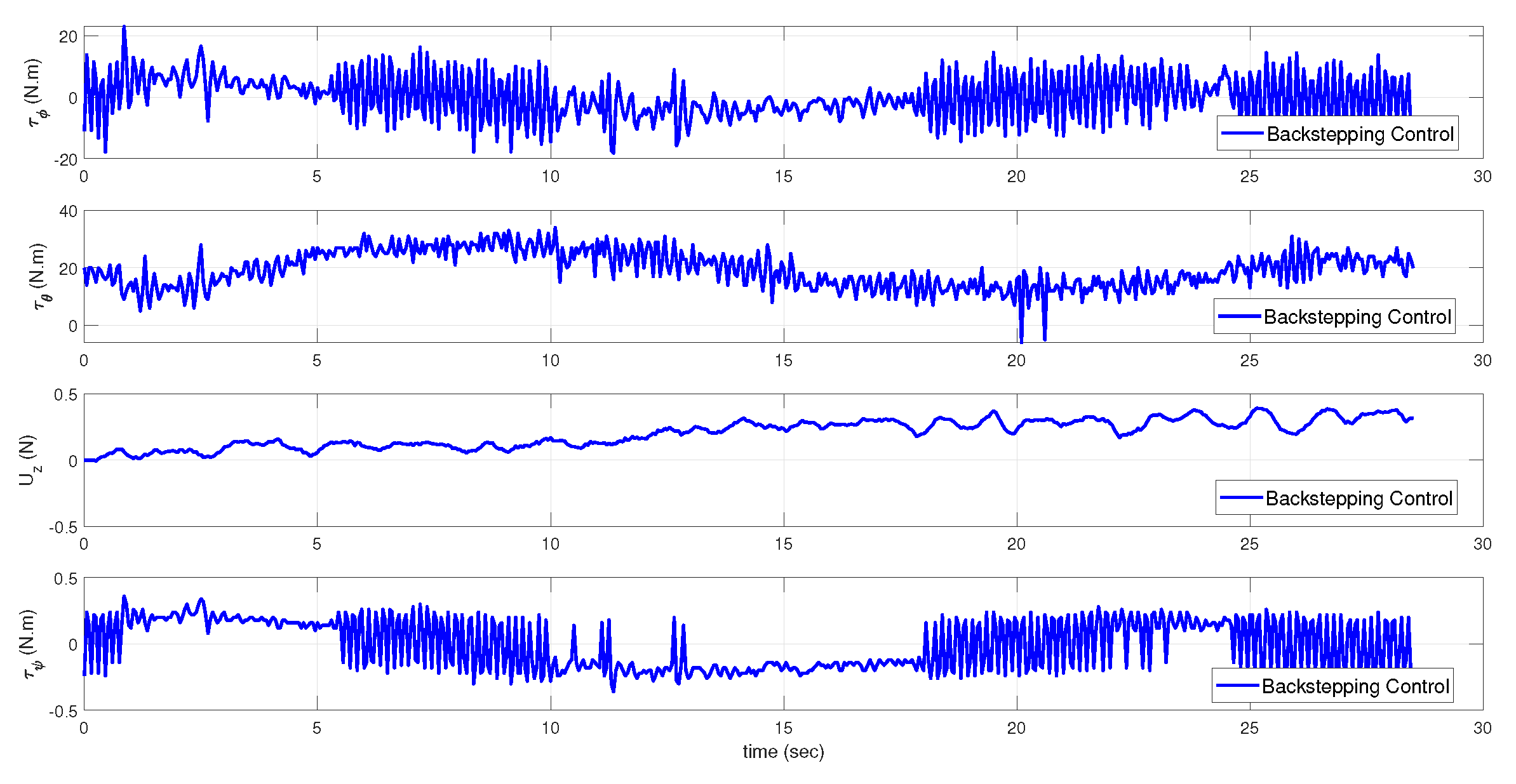
- A new robust backstepping approach-based control algorithm that considers matched vanishing disturbances is proposed. The proposed controller uses a virtual bounded input: the function , which produces bounded control signals, and it is appropriate to the physical constrains of the UAV.
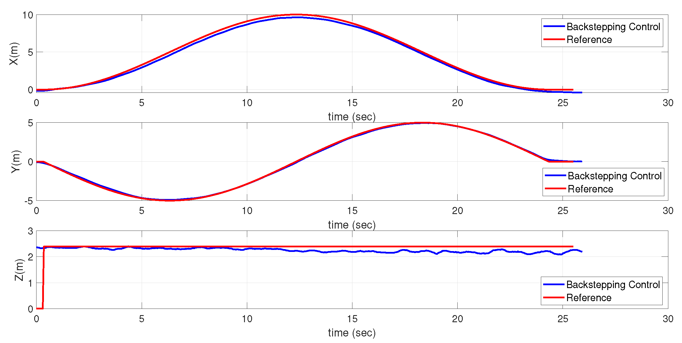
- Experimental results in trajectory tracking using a UAV in an outdoor environment are reported. A specific precision agriculture task is involved using a commercial camera system and MATLAB software.
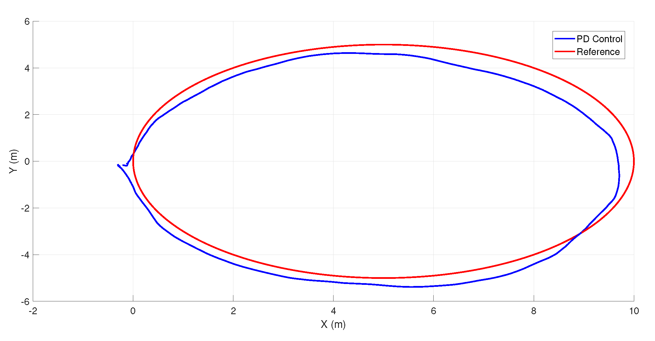
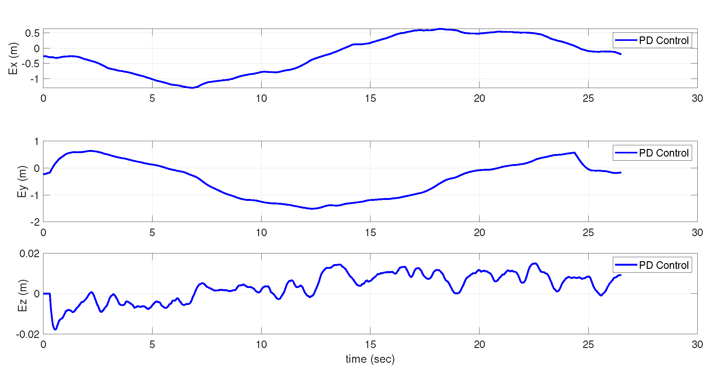
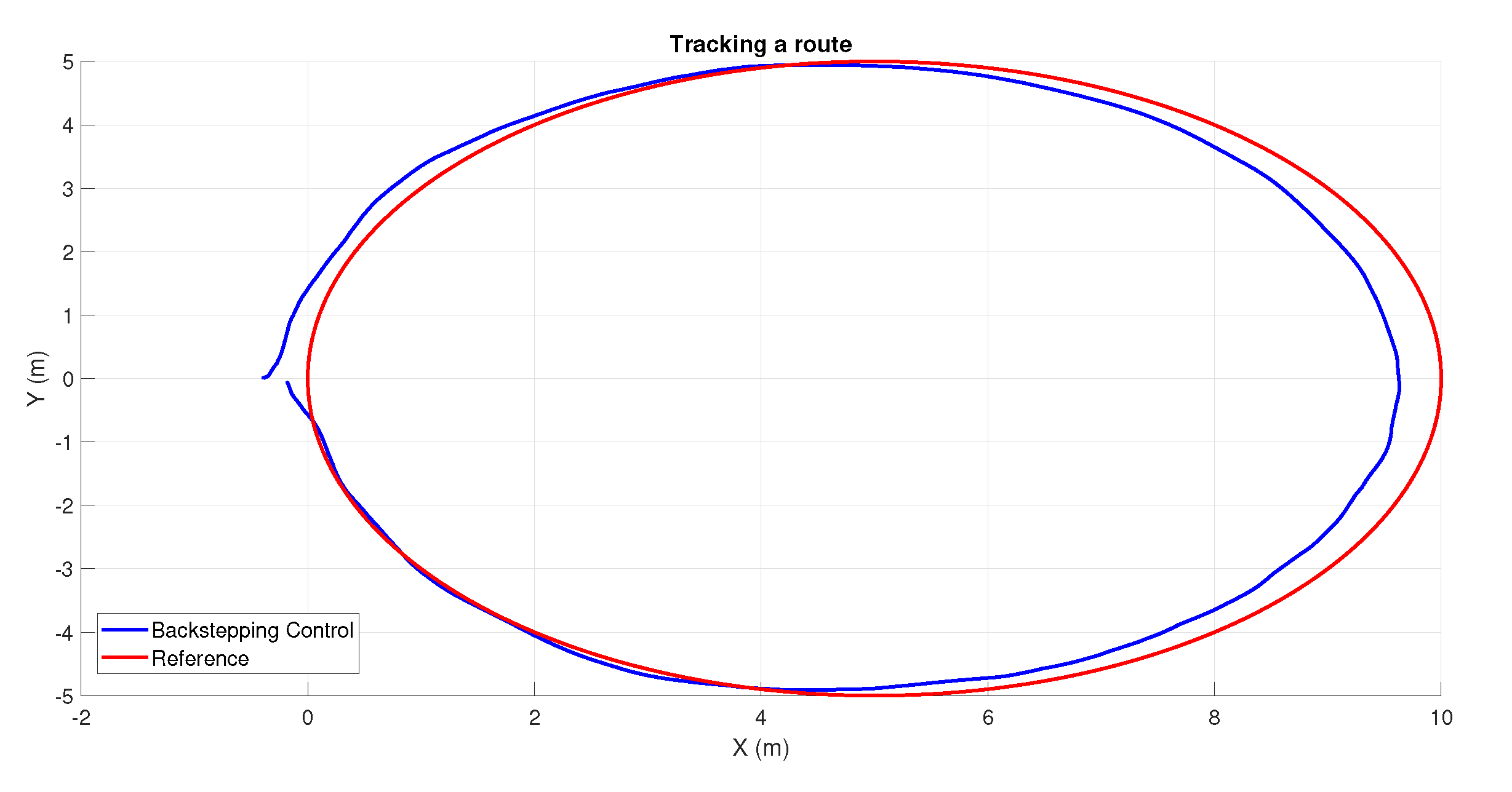
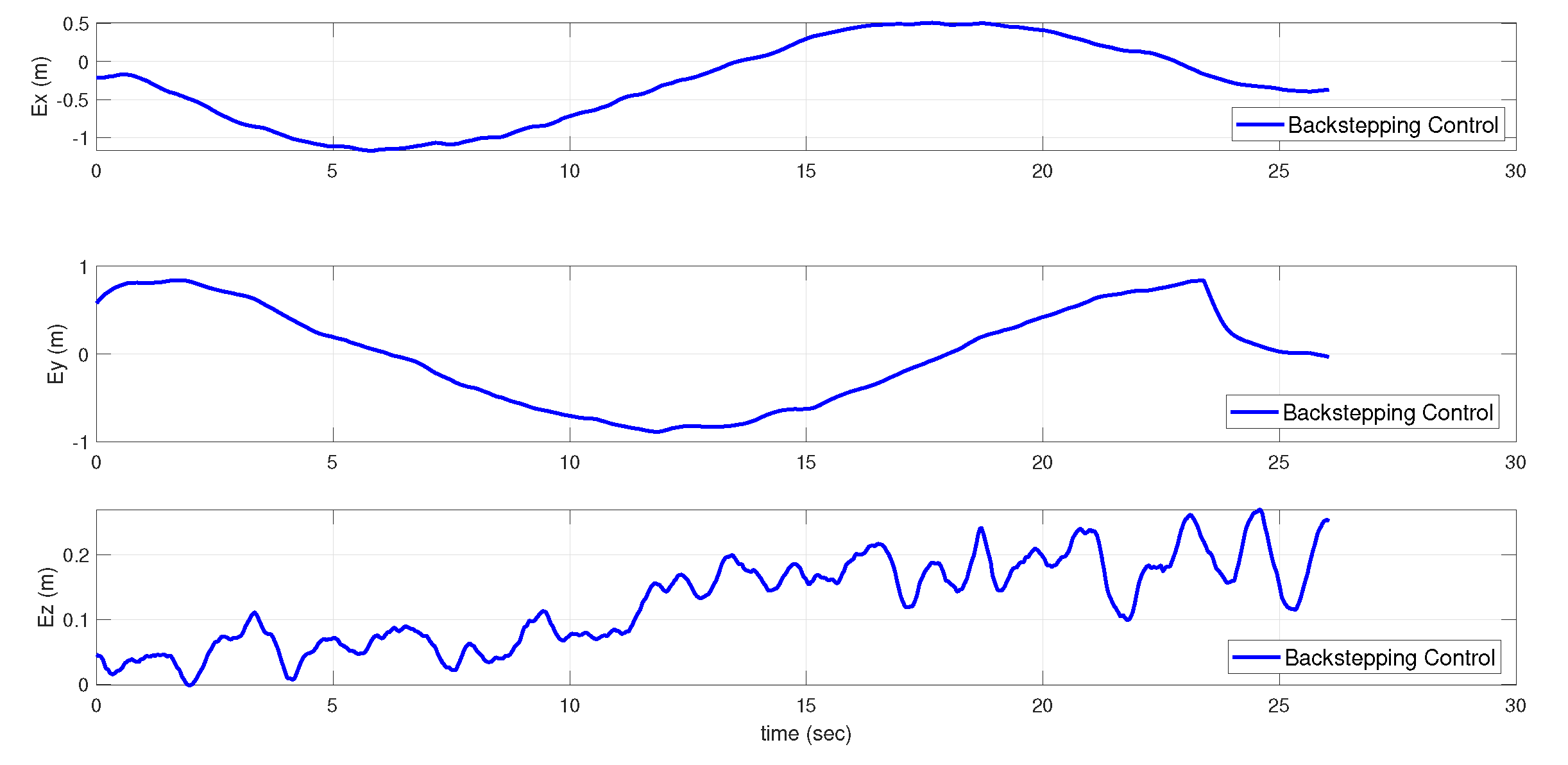
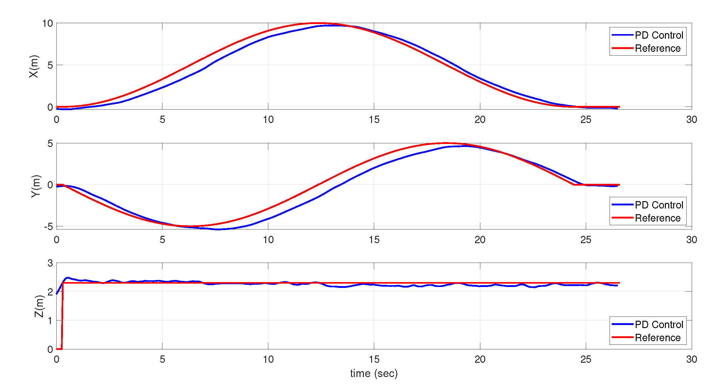
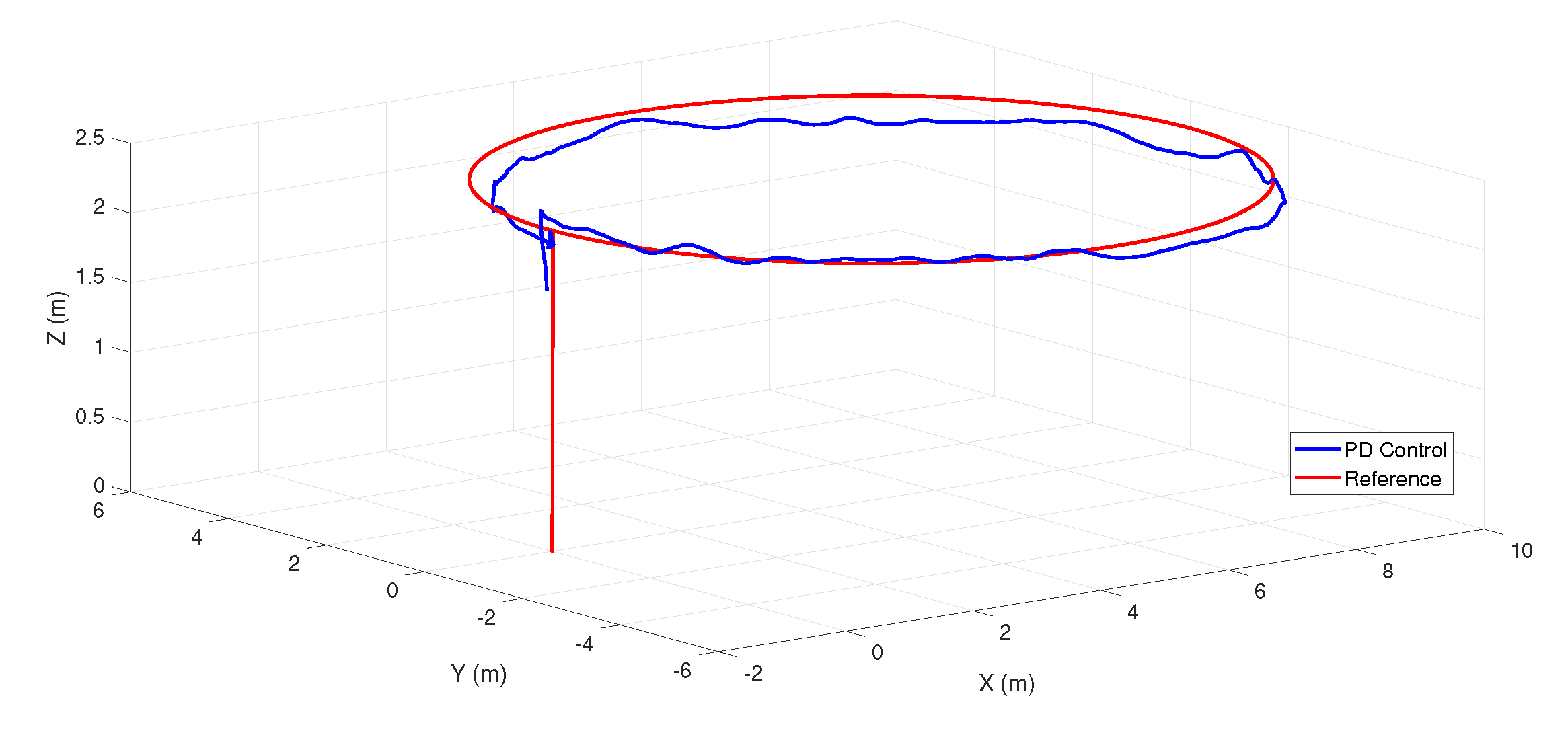
- The robustness provided to the proposed controller allows to reduce the capture of distorted crop images and it represents better performance when our proposal is compared to a PD controller, although a gimbal or additional software are not used.
- This article tries to fill the gap between the technological development with advanced control theory.
2. Problem Formulation and Main Results
2.1. System Description
- The known functions and are continuously differentiable in a domain that contains the origin and .
- The Equation (1) of the system can be stabilized with a state feedback with , then, there is a Lyapunov function that satisfies the following equation:where is a positive definite function,
- Function is a bounded matched vanishing perturbation, i.e.,
2.2. Main Result
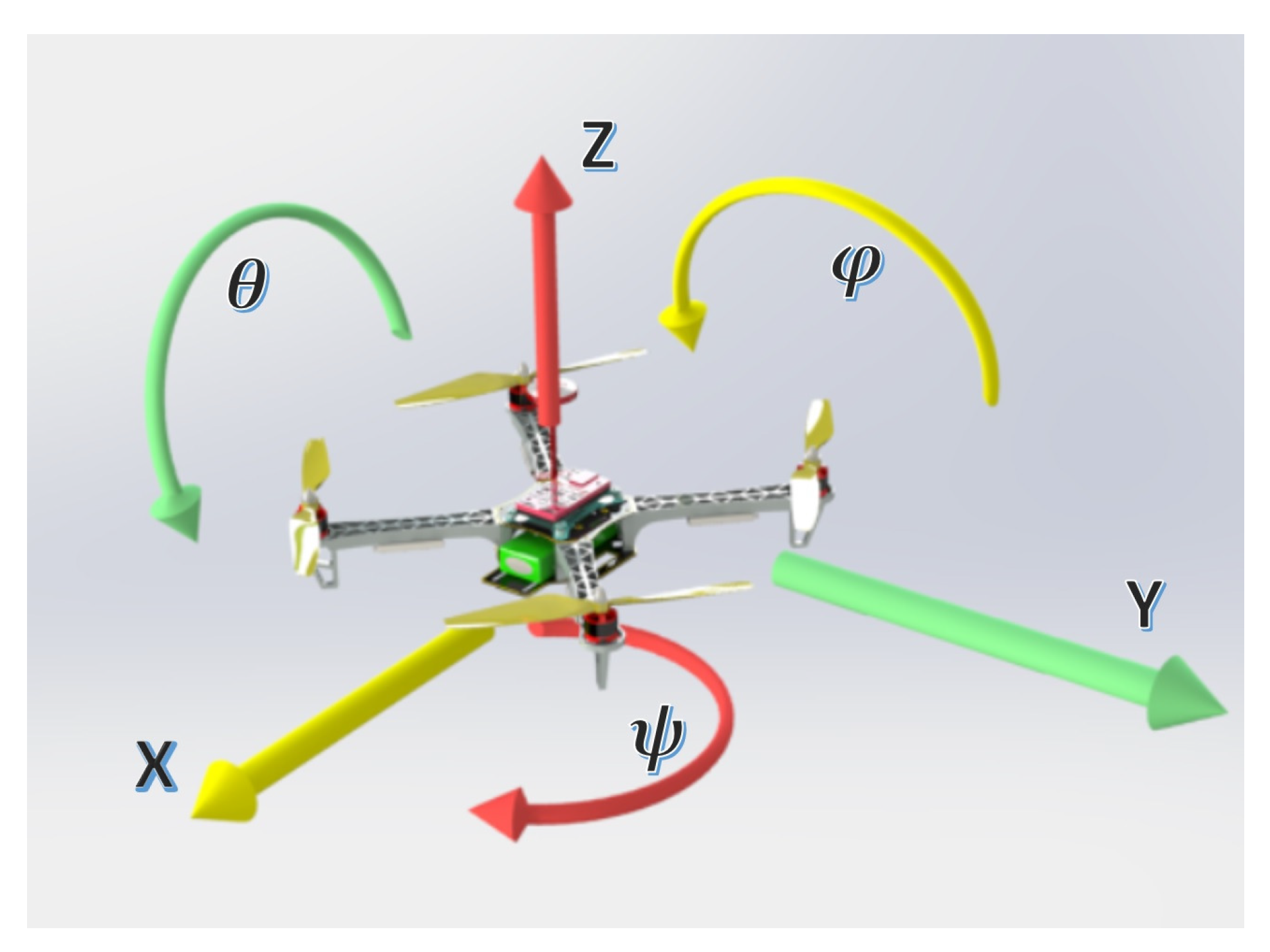
3. Quadrotor Model
- The UAV is considered as a rigid and symmetrical body.
- The center of gravity (CoG) of the quadrotor is in its origin.
- The blades are rigid bodies with fixed angle pitch.
- In the nominal model of the quadrotor, the aerodynamics effects have not been considered.
- The motor dynamic could be modeled as a first-order transfer function, and it is sufficient to reproduce the dynamics between the propeller’s speed set-point and its true speed. As the time constant of this transfer function is small, we can consider that the rotor dynamic is approximately equal to one [33]. This assumption is used to suppose additional dynamics (or uncertain parameters) that represent matched vanishing perturbations in the actuators.
- The attitude angles, pitch, roll and yaw are restricted in the interval [, ].
4. Control Strategy Applied to the Quadrotor
4.1. Altitude Controller
4.2. Yaw Controller
4.3. Controller for Subsystem
4.4. Controller for Subsystem
5. Experimental Results
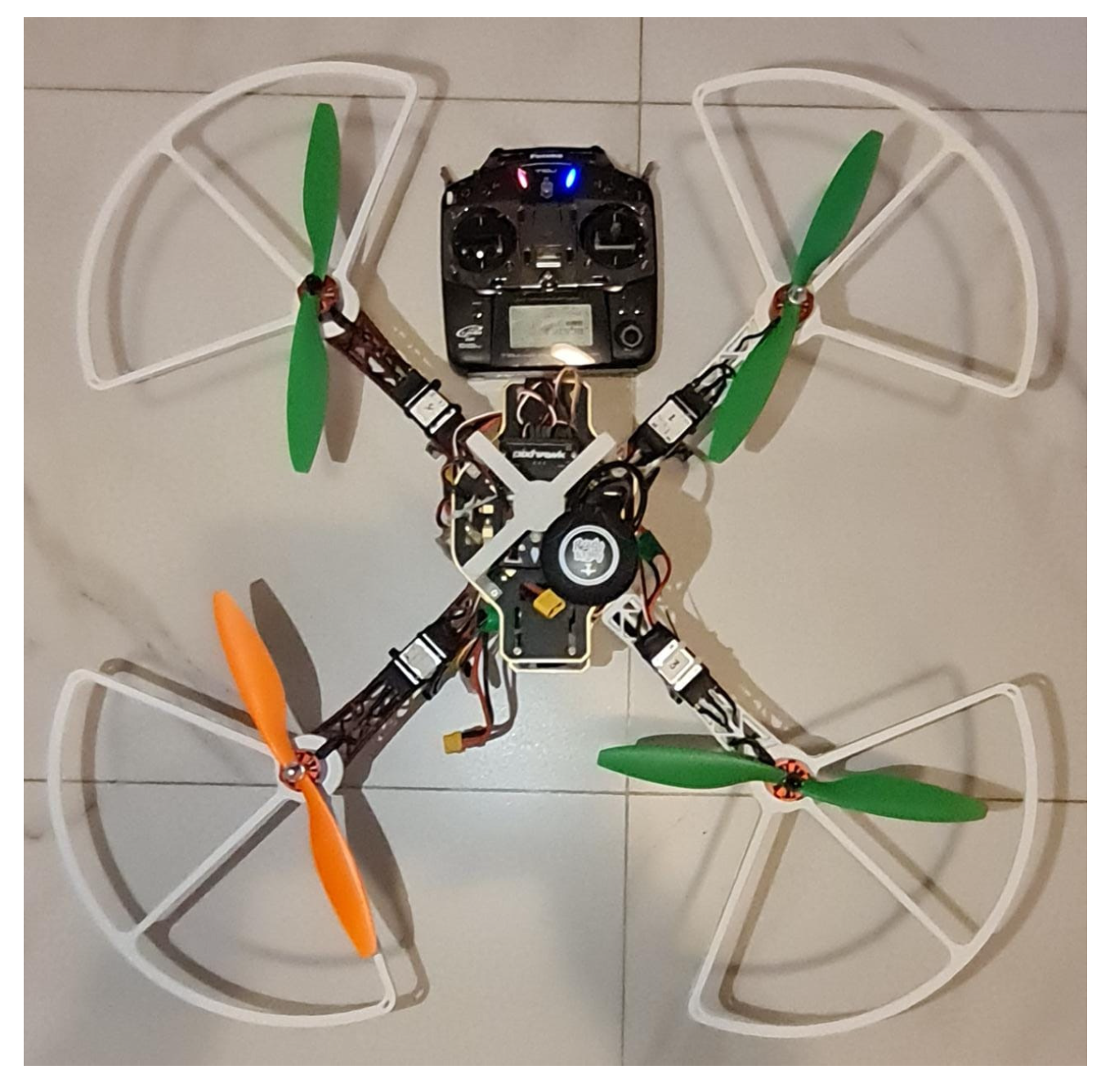
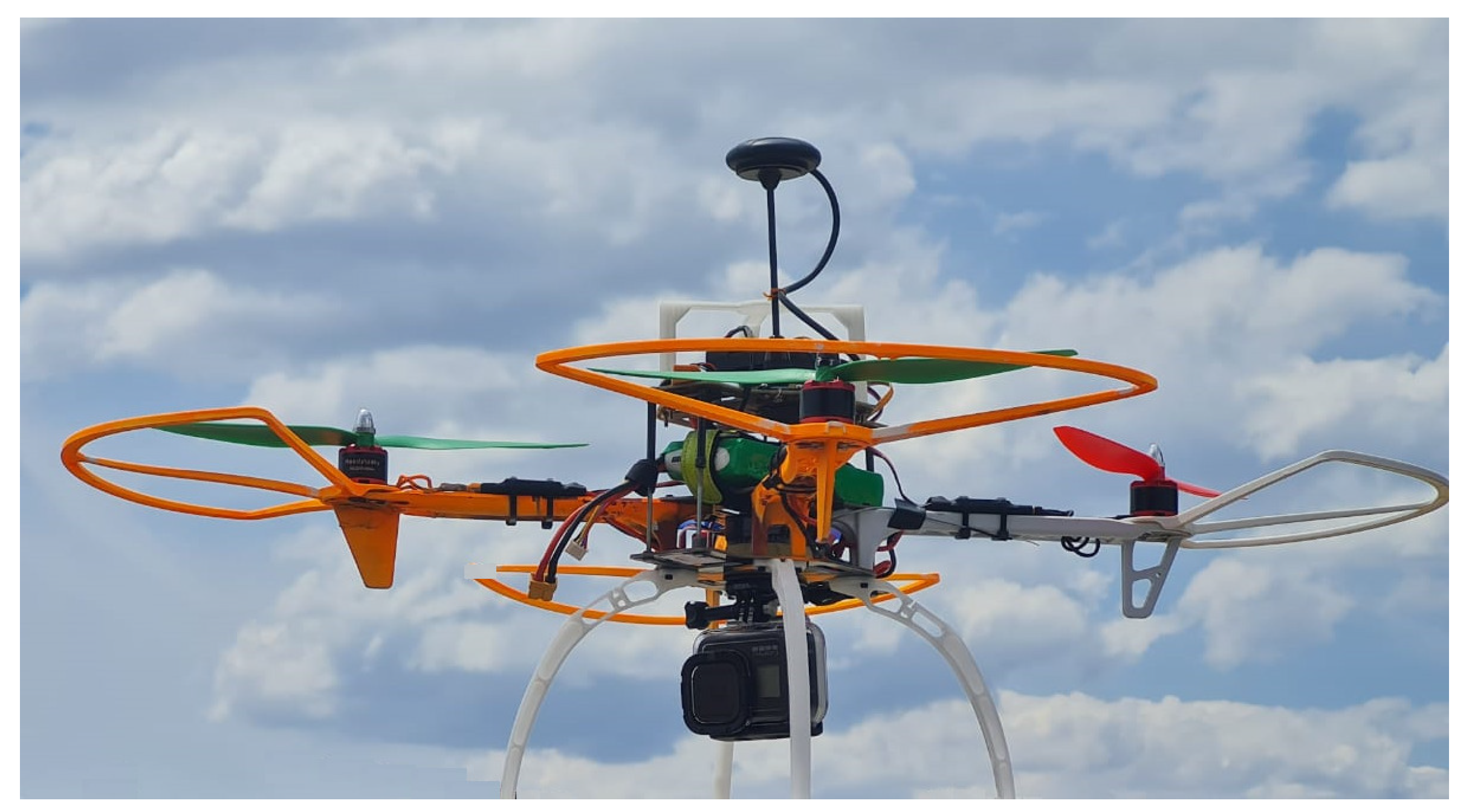
5.1. Experimental Platform Description
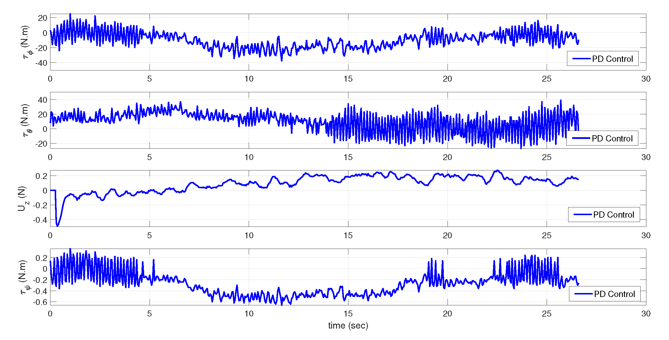
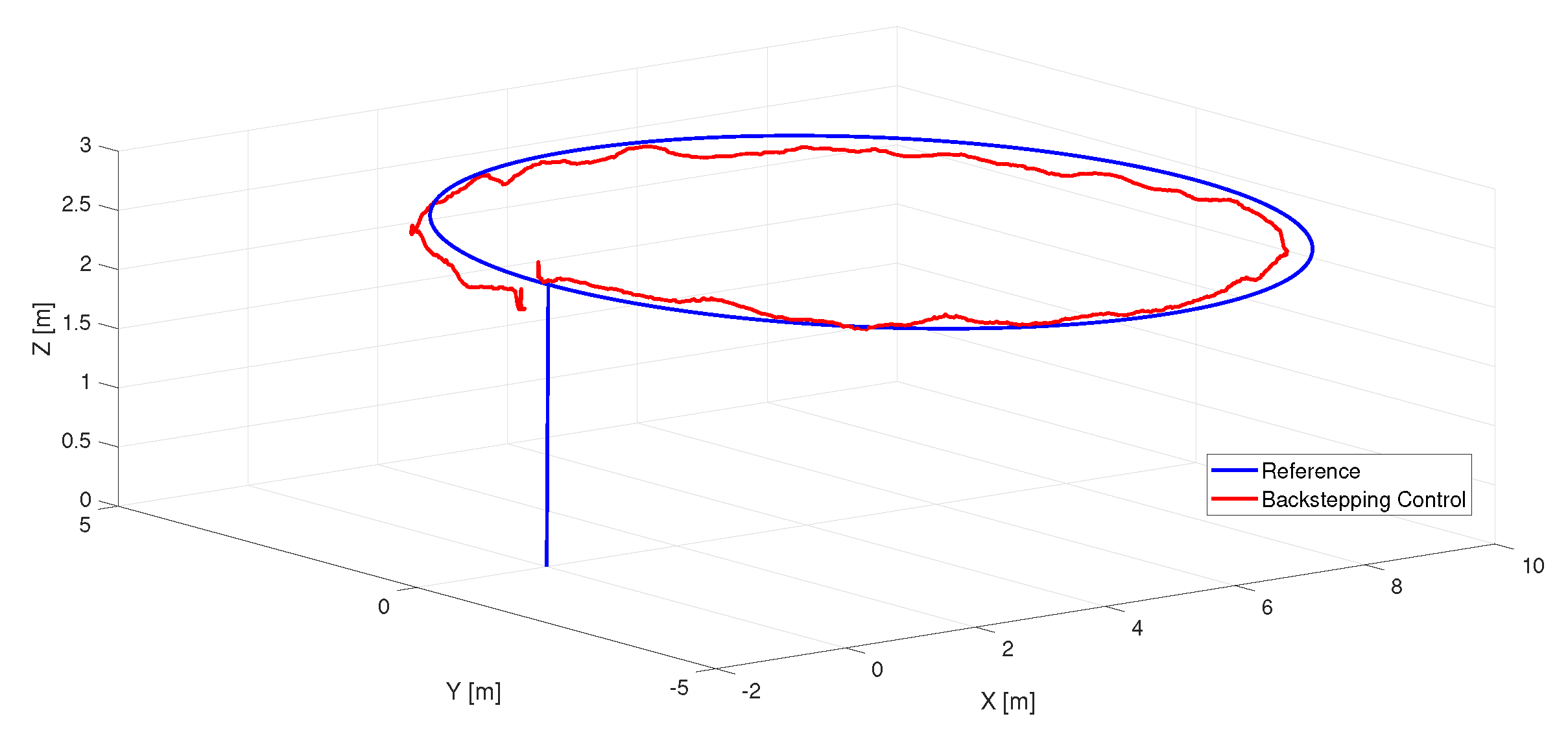
5.2. Experimental Results Applying Synthesized Controllers
6. Detection of Pest in Corn Leaves
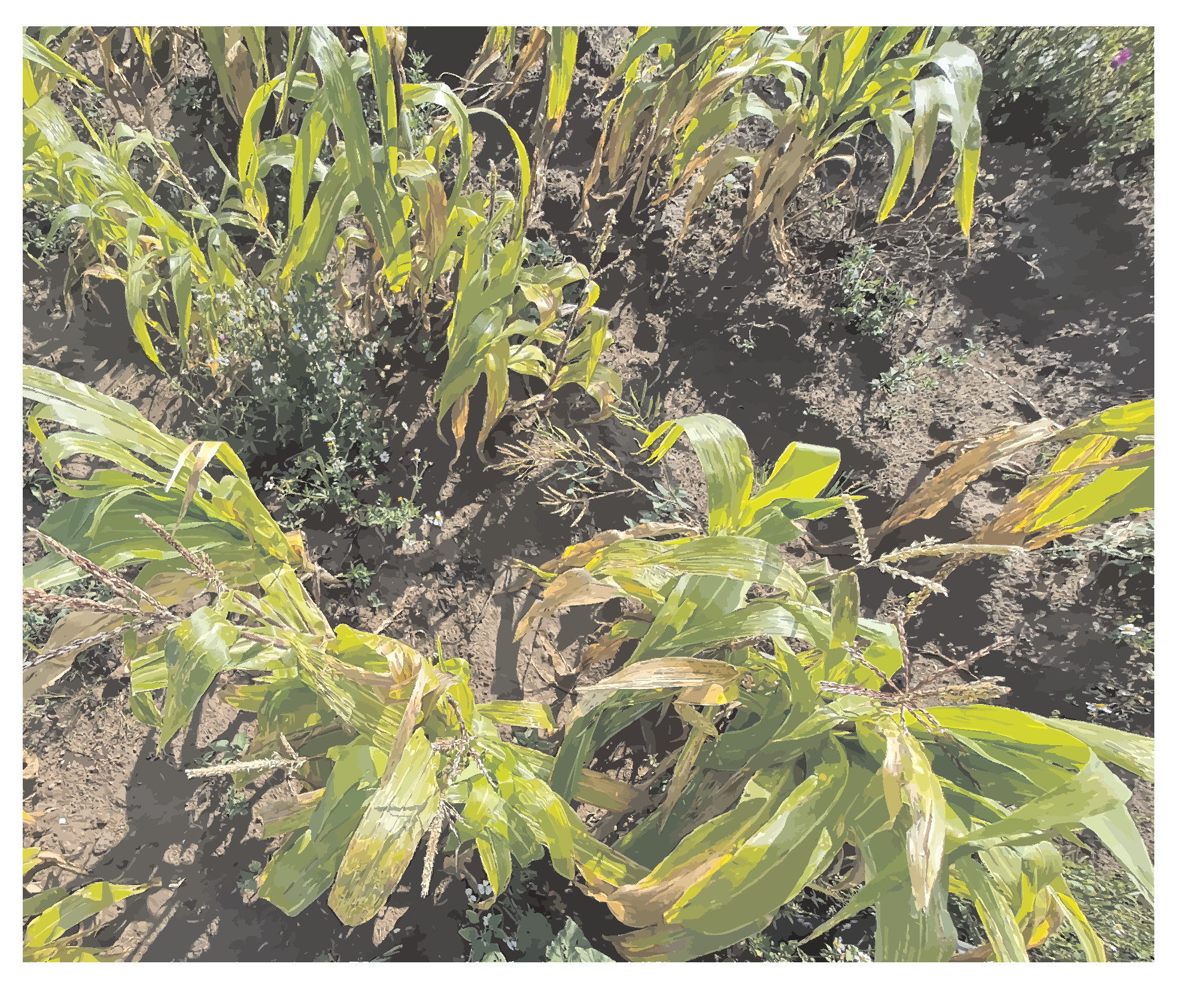
6.1. Vision System
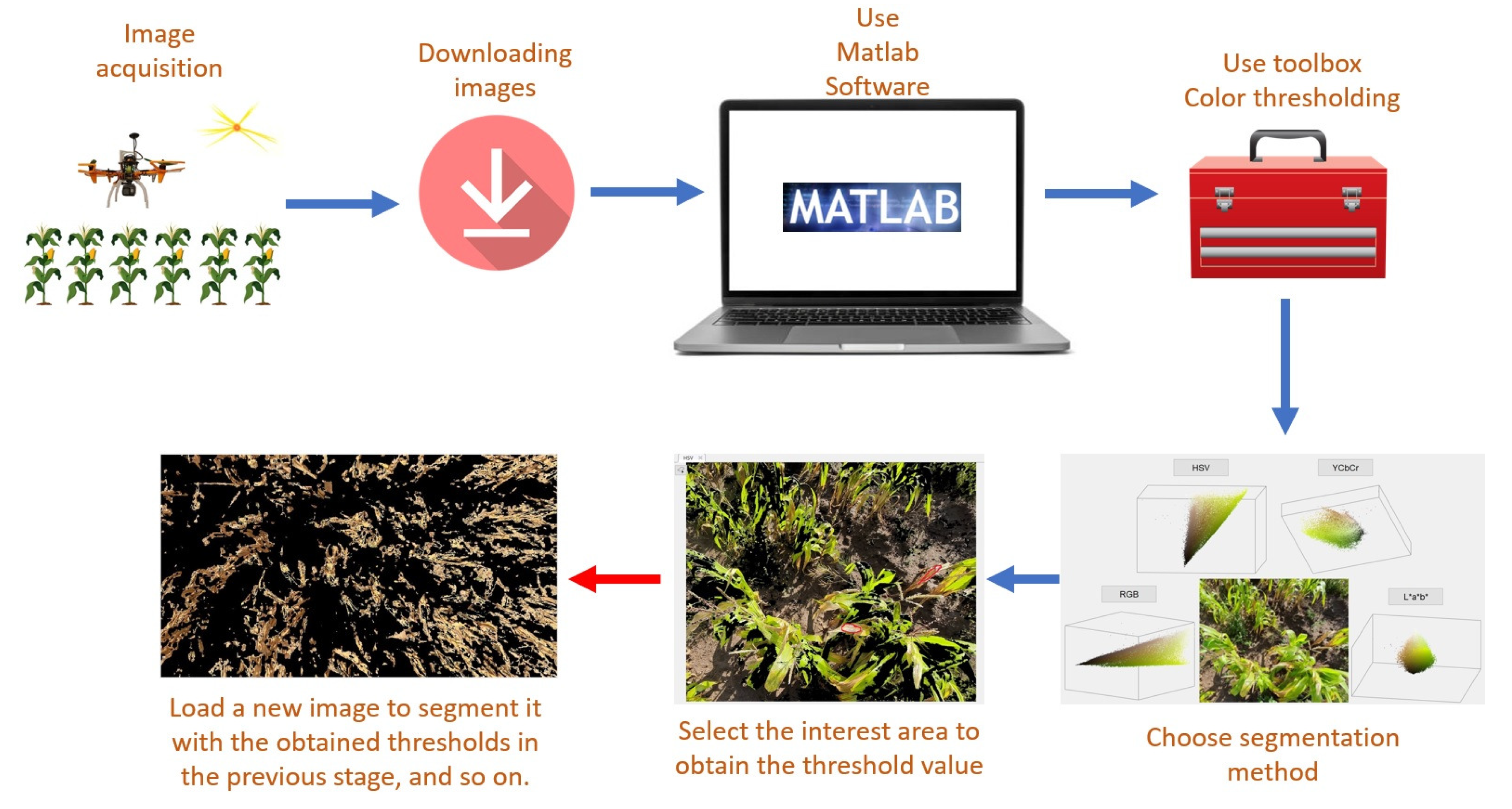
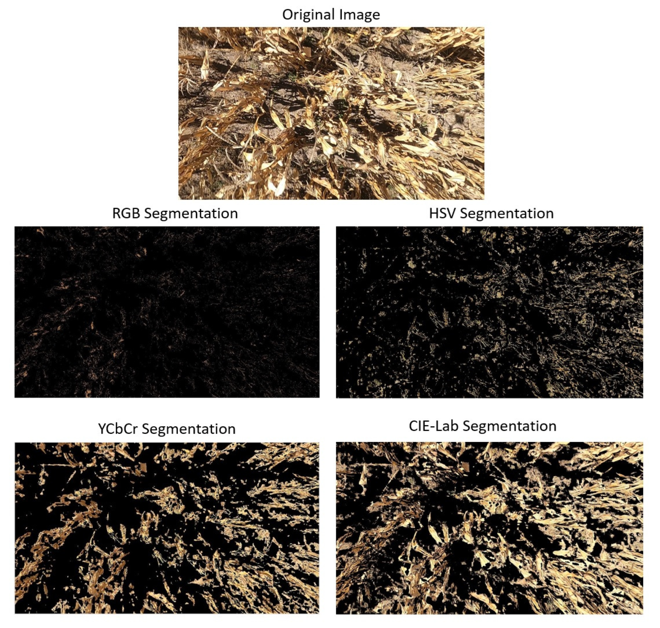
6.2. Image Processing
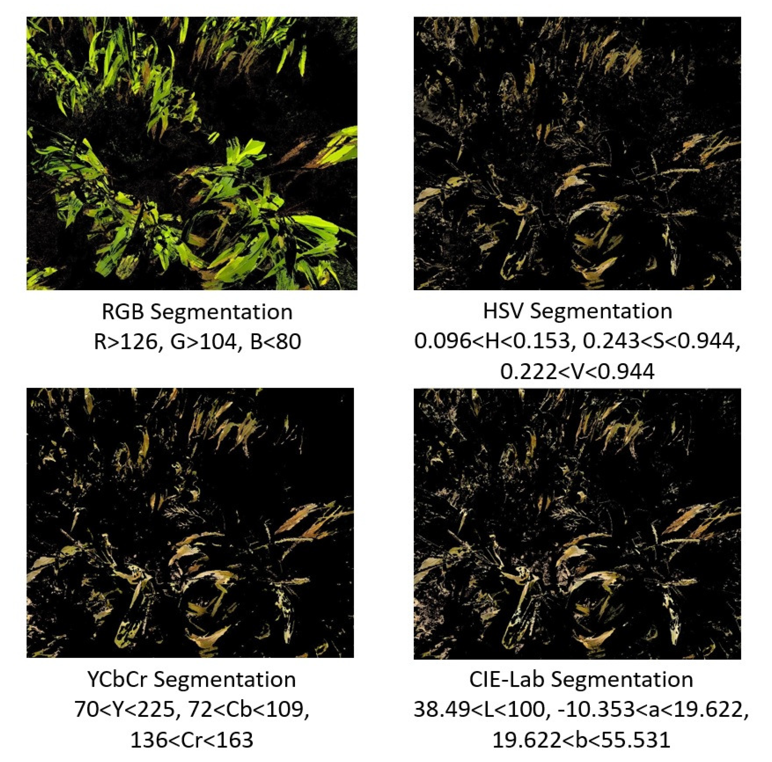
Segmentation Method
7. Conclusions
Author Contributions
Funding
Institutional Review Board Statement
Informed Consent Statement
Data Availability Statement
Conflicts of Interest
References
- Thanh, H.L.N.N.; Hong, S.K. Quadcopter robust adaptive second order sliding mode control based on PID sliding surface. IEEE Access 2018, 6, 66850–66860. [Google Scholar] [CrossRef]
- Ononiwu, G.; Onojo, O.; Ozioko, O.; Nosiri, O. Quadcopter design for payload delivery. J. Comput. Commun. 2016, 4, 1–12. [Google Scholar] [CrossRef]
- Duggal, V.; Sukhwani, M.; Bipin, K.; Syamasundar Reddy, G.; Madhava Krishna, K. Plantation monitoring and yield estimation using autonomous quadcopter for precision agriculture. In Proceedings of the 2016 IEEE International Conference on Robotics and Automation (ICRA), Stockholm, Sweden, 16–21 May 2016; pp. 5121–5127. [Google Scholar]
- Mogili, U.R.; Deepak, B. Review on application of drone systems in precision agriculture. Procedia Comput. Sci. 2018, 133, 502–509. [Google Scholar] [CrossRef]
- Kuantama, E.; Tarca, R.; Dzitac, S.; Dzitac, I.; Vesselenyi, T.; Tarca, I. The design and experimental development of air scanning using a sniffer Quadcopter. Sensors 2019, 19, 3849. [Google Scholar] [CrossRef] [PubMed]
- Rudin, K.; Hua, M.D.; Ducard, G.; Bouabdallah, S. A robust attitude controller and its application to quadrotor helicopters. IFAC Proc. Vol. 2011, 44, 10379–10384. [Google Scholar] [CrossRef]
- Ramirez-Rodriguez, H.; Parra-Vega, V.; Sanchez-Orta, A.; Garcia-Salazar, O. Robust backstepping control based on integral sliding modes for tracking of quadrotors. J. Intell. Robot. Syst. 2014, 73, 55–66. [Google Scholar] [CrossRef]
- Peng, C.; Bai, Y.; Gong, X.; Gao, Q.; Zhao, C.; Tian, Y. Modeling and robust backstepping sliding mode control with Adaptive RBFNN for a novel coaxial eight-rotor UAV. IEEE/CAA J. Autom. Sin. 2015, 2, 56–64. [Google Scholar]
- Zhao, Y.; Sun, X.; Wang, G.; Fan, Y. Adaptive Backstepping Sliding Mode Tracking Control for Underactuated Unmanned Surface Vehicle With Disturbances and Input Saturation. IEEE Access 2021, 9, 1304–1312. [Google Scholar] [CrossRef]
- Kim, N.S.; Kuc, T.Y. Sliding Mode Backstepping Control for Variable Mass Hexa-Rotor UAV. In Proceedings of the 2020 20th International Conference on Control, Automation and Systems (ICCAS), Busan, Korea, 13–16 October 2020; pp. 873–878. [Google Scholar]
- García, O.; Ordaz, P.; Santos-Sánchez, O.J.; Salazar, S.; Lozano, R. Backstepping and Robust Control for a Quadrotor in Outdoors Environments: An Experimental Approach. IEEE Access 2019, 7, 40635–40648. [Google Scholar] [CrossRef]
- Colorado, J.D.; Cera-Bornacelli, N.; Caldas, J.S.; Petro, E.; Rebolledo, M.C.; Cuellar, D.; Calderon, F.; Mondragon, I.F.; Jaramillo-Botero, A. Estimation of nitrogen in rice crops from UAV-captured images. Remote Sens. 2020, 12, 3396. [Google Scholar] [CrossRef]
- Cabecinhas, D.; Cunha, R.; Silvestre, C. A nonlinear quadrotor trajectory tracking controller with disturbance rejection. Control Eng. Pract. 2014, 26, 1–10. [Google Scholar] [CrossRef]
- Vallejo-Alarcón, M.A.; Castro-Linares, R. Robust backstepping control for highly demanding quadrotor flight. Control Eng. Appl. Inform. 2020, 22, 51–62. [Google Scholar]
- Aboudonia, A.; El-Badawy, A.; Rashad, R. Active anti-disturbance control of a quadrotor unmanned aerial vehicle using the command-filtering backstepping approach. Nonlinear Dyn. 2017, 90, 581–597. [Google Scholar] [CrossRef]
- Zhang, J.; Gu, D.; Deng, C.; Wen, B. Robust and adaptive backstepping control for hexacopter UAVs. IEEE Access 2019, 7, 163502–163514. [Google Scholar] [CrossRef]
- Dhadekar, D.D.; Sanghani, P.D.; Mangrulkar, K.; Talole, S. Robust control of quadrotor using uncertainty and disturbance estimation. J. Intell. Robot. Syst. 2021, 101, 1–21. [Google Scholar] [CrossRef]
- Xuan-Mung, N.; Hong, S.K.; Nguyen, N.P.; Le, T.L. Autonomous quadcopter precision landing onto a heaving platform: New method and experiment. IEEE Access 2020, 8, 167192–167202. [Google Scholar] [CrossRef]
- Derrouaoui, S.H.; Bouzid, Y.; Guiatni, M. Nonlinear robust control of a new reconfigurable unmanned aerial vehicle. Robotics 2021, 10, 76. [Google Scholar] [CrossRef]
- de Morais, G.A.; Marcos, L.B.; Bueno, J.N.A.; de Resende, N.F.; Terra, M.H.; Grassi, V., Jr. Vision-based robust control framework based on deep reinforcement learning applied to autonomous ground vehicles. Control Eng. Pract. 2020, 104, 104630. [Google Scholar] [CrossRef]
- Castillo, P.; Munoz, L.; Santos, O. Robust control algorithm for a rotorcraft disturbed by crosswind. IEEE Trans. Aerosp. Electron. Syst. 2014, 50, 756–763. [Google Scholar] [CrossRef]
- Li, C.; Zhang, Y.; Li, P. Full control of a quadrotor using parameter-scheduled backstepping method: Implementation and experimental tests. Nonlinear Dyn. 2017, 89, 1259–1278. [Google Scholar] [CrossRef]
- Mokhtari, M.R.; Cherki, B. A new robust control for minirotorcraft unmanned aerial vehicles. ISA Trans. 2015, 56, 86–101. [Google Scholar] [CrossRef] [PubMed]
- Mejias, L.; Diguet, J.P.; Dezan, C.; Campbell, D.; Kok, J.; Coppin, G. Embedded computation architectures for autonomy in Unmanned Aircraft Systems (UAS). Sensors 2021, 21, 1115. [Google Scholar] [CrossRef] [PubMed]
- López-Labra, H.A.; Santos-Sánchez, O.J.; Rodríguez-Guerrero, L.; Ordaz-Oliver, J.P.; Cuvas-Castillo, C. Experimental results of optimal and robust control for uncertain linear time-delay systems. J. Optim. Theory Appl. 2019, 181, 1076–1089. [Google Scholar] [CrossRef]
- Khalil, H.K. Nonlinear Systems, 3rd ed.; Prentice Hall: Hoboken, NJ, USA, 1996. [Google Scholar]
- Hock, J.; Kranz, J.; Renfro, B. Studies on the epidemiology of the tar spot disease complex of maize in Mexico. Plant Pathol. 1995, 44, 490–502. [Google Scholar] [CrossRef]
- Velusamy, P.; Rajendran, S.; Mahendran, R.K.; Naseer, S.; Shafiq, M.; Choi, J.G. Unmanned Aerial Vehicles (UAV) in precision agriculture: Applications and challenges. Energies 2021, 15, 217. [Google Scholar] [CrossRef]
- Kitpo, N.; Inoue, M. Early rice disease detection and position mapping system using drone and IoT architecture. In Proceedings of the 2018 12th South East Asian Technical University Consortium (SEATUC), Yogyakarta, Indonesia, 12–13 March 2018; Volume 1, pp. 1–5. [Google Scholar]
- Görlich, F.; Marks, E.; Mahlein, A.K.; König, K.; Lottes, P.; Stachniss, C. UAV-based classification of cercospora leaf spot using RGB images. Drones 2021, 5, 34. [Google Scholar] [CrossRef]
- Castillo, P.; Lozano, R.; Dzul, A. Modelling and Control of Mini-Flying Machines, 1st ed.; Springer: London, UK, 2005. [Google Scholar]
- Lozano, R. Unmanned Aerial Vehicles: Embedded Control, 1st ed.; Wiley-ISTE: London, UK, 2010. [Google Scholar]
- Bouabdallah, S.; Siegwart, R. Full control of a quadrotor. In Proceedings of the 2007 IEEE/RSJ International Conference on Intelligent Robots and Systems, San Diego, CA, USA, 29 October–2 November 2007; pp. 153–158. [Google Scholar]
- Svacha, J.; Mohta, K.; Kumar, V. Improving quadrotor trajectory tracking by compensating for aerodynamic effects. In Proceedings of the 2017 International Conference on Unmanned Aircraft Systems (ICUAS), Miami, FL, USA, 13–16 June 2017; pp. 860–866. [Google Scholar]
- Santos, O.; Romero, H.; Salazar, S.; Garcia, O. Optimized Discrete Control Law for Quadrotor Stabilization: Experimental Results. J. Intell. Robot. Syst. 2016, 84, 67–81. [Google Scholar] [CrossRef]
- GoPro-Cameras. GoPro Inc. June 2022. Available online: https://gopro.com/en/us/shop/cameras/hero8-black/CHDHX801-master.html (accessed on 30 June 2022).
- Kaganami, H.G.; Beiji, Z. Region-based segmentation versus edge detection. In Proceedings of the 2009 Fifth International Conference on Intelligent Information Hiding and Multimedia Signal Processing, Kyoto, Japan, 12–14 September 2009; pp. 1217–1221. [Google Scholar]


| Subsystems | |||
|---|---|---|---|
| Trajectory Tracking | ||||
|---|---|---|---|---|
| Performance Index | BS | PD | ||
| IAEx | 674.0325 | 732.8948 | 0.3195 | 0.6095 |
| IAEy | 646.48 | 849.0646 | 0.5691 | 0.6949 |
| IAEz | 59.96 | 85.4140 | 0.06747 | 0.0678 |
| Trajectory Tracking | ||
|---|---|---|
| Performance Index | BS | PD |
| 6051.2 | 6662 | |
| 7337 | 8661 | |
| 519.647 | 662.5175 | |
| 802.8 | 848.2 | |
Publisher’s Note: MDPI stays neutral with regard to jurisdictional claims in published maps and institutional affiliations. |
© 2022 by the authors. Licensee MDPI, Basel, Switzerland. This article is an open access article distributed under the terms and conditions of the Creative Commons Attribution (CC BY) license (https://creativecommons.org/licenses/by/4.0/).
Share and Cite
Rodríguez-Guerrero, L.; Benítez-Morales, A.; Santos-Sánchez, O.-J.; García-Pérez, O.; Romero-Trejo, H.; Ordaz-Oliver, M.-O.; Ordaz-Oliver, J.-P. Robust Backstepping Control Applied to UAVs for Pest Recognition in Maize Crops. Appl. Sci. 2022, 12, 9075. https://doi.org/10.3390/app12189075
Rodríguez-Guerrero L, Benítez-Morales A, Santos-Sánchez O-J, García-Pérez O, Romero-Trejo H, Ordaz-Oliver M-O, Ordaz-Oliver J-P. Robust Backstepping Control Applied to UAVs for Pest Recognition in Maize Crops. Applied Sciences. 2022; 12(18):9075. https://doi.org/10.3390/app12189075
Chicago/Turabian StyleRodríguez-Guerrero, Liliam, Alejandro Benítez-Morales, Omar-Jacobo Santos-Sánchez, Orlando García-Pérez, Hugo Romero-Trejo, Mario-Oscar Ordaz-Oliver, and Jesús-Patricio Ordaz-Oliver. 2022. "Robust Backstepping Control Applied to UAVs for Pest Recognition in Maize Crops" Applied Sciences 12, no. 18: 9075. https://doi.org/10.3390/app12189075
APA StyleRodríguez-Guerrero, L., Benítez-Morales, A., Santos-Sánchez, O.-J., García-Pérez, O., Romero-Trejo, H., Ordaz-Oliver, M.-O., & Ordaz-Oliver, J.-P. (2022). Robust Backstepping Control Applied to UAVs for Pest Recognition in Maize Crops. Applied Sciences, 12(18), 9075. https://doi.org/10.3390/app12189075