Effect of Soil Damping on the Soil–Pile–Structure Interaction Analyses in Cohesionless Soils

Abstract

Pile foundations in earthquake-prone regions must be analyzed and designed considering the dynamic loads. In the fully nonlinear dynamic analyses, the soil nonlinearity can be considered using the modulus degradation curves in the total-stress approach, and the soil damping is controlled by the unloading/reloading rule. Several researchers have investigated the effect of soil damping on the free-field soil response analyses, but the effect on the soil–pile–structure system response has not been studied thoroughly. In this study, the nonlinear elastic method (hyperbolic model) and the elastoplastic Mohr–Coulomb (MC) models were implemented to investigate the effect of soil damping on the pile and structure response. Dynamic soil–pile–structure interaction analyses were performed by simulating two different centrifuge tests published in the literature, and the analysis results were compared with the centrifuge test results. The analyses with the low-intensity input motions showed that the superstructure accelerations and the bending moments in the single pile were estimated with reasonable accuracy. However, the superstructure accelerations might be underestimated under high-intensity motions, especially in the MC model. Additional analyses were performed under six earthquake records. The constitutive models (MC and hyperbolic) may significantly vary the maximum structural acceleration and pile maximum moments (up to 50%). As a result, the responses of the superstructure and the pile in soil–pile–structure interaction problems are highly dependent on the soil constitutive model that must take the damping into account accurately; in turn, due account must be given to the selection of the constitutive model.

1. Introduction

Designing a pile foundation is critical under lateral loading, especially in high seismicity zones. Two commonly used methods are available for the analyses: Three-dimensional finite element (or finite difference) [1,2,3,4] or beam on Winkler Foundation (BNWF) [5,6,7] approaches. Both methods require the definition of nonlinear soil behavior under dynamic loads. Historically, the assumption of linear behavior for the pile and the superstructure is valid in most cases, and the linear soil–pile–structure interaction has been well studied by various researchers [8,9,10]. However, soils exhibit highly nonlinear behavior even under low strains, and the main uncertainty in the analyses arises from the modeling approach taking this nonlinearity into account [7,11,12,13].

The nonlinear behavior of soils has been studied by many researchers experimentally [14,15,16,17,18]. The equivalent-linear analysis method was developed initially [19], and the modulus degradation curves have expressed the soil nonlinearity in these analyses. The equivalent-linear analysis is a theoretically linear method, but the soil nonlinearity and damping are integrated into the analyses by an iterative approach. The fully nonlinear techniques have been developed to represent the nonlinear soil behavior accurately. However, a major difficulty in the fully nonlinear methods is the definition of unloading/reloading behavior which governs the damping ratio. The effect of several soil constitutive models on the soil response has been studied by 1-dimensional site response analyses [20,21,22,23]. Several other 3D constitutive models are available to simulate soil behavior [24,25,26]. However, a wide variety of damping performances exist under dynamic loading. Studies have been conducted on the soil–pile–structure interaction [2,27,28,29]. However, the effect of soil damping on the structure and pile responses has not been studied thoroughly.

The main purpose of this study is to show the effect of the soil hysteretic damping on the pile–soil–structure system response using relatively simple constitutive models. Two different centrifuge test setups of Gohl [30] and Wilson [31] were simulated by three-dimensional models in FLAC^3D [32] for verification purposes. Fully nonlinear analyses were performed for the single pile–soil–structure systems. Since the earthquake records used in the centrifuge tests were limited, a new numerical model was created, having a single pile–structure model embedded in a single cohesionless soil layer and analyzed using six different earthquake records. The methods followed in the study are given in detail in Section 2. The results of the analyses are presented in Section 3.

2. The Method

The main objective of this study is to show the effect of soil’s damping ratio on the soil–pile–structure interaction analyses. For this purpose, two constitutive models were employed; each has a different damping formulation for soil.

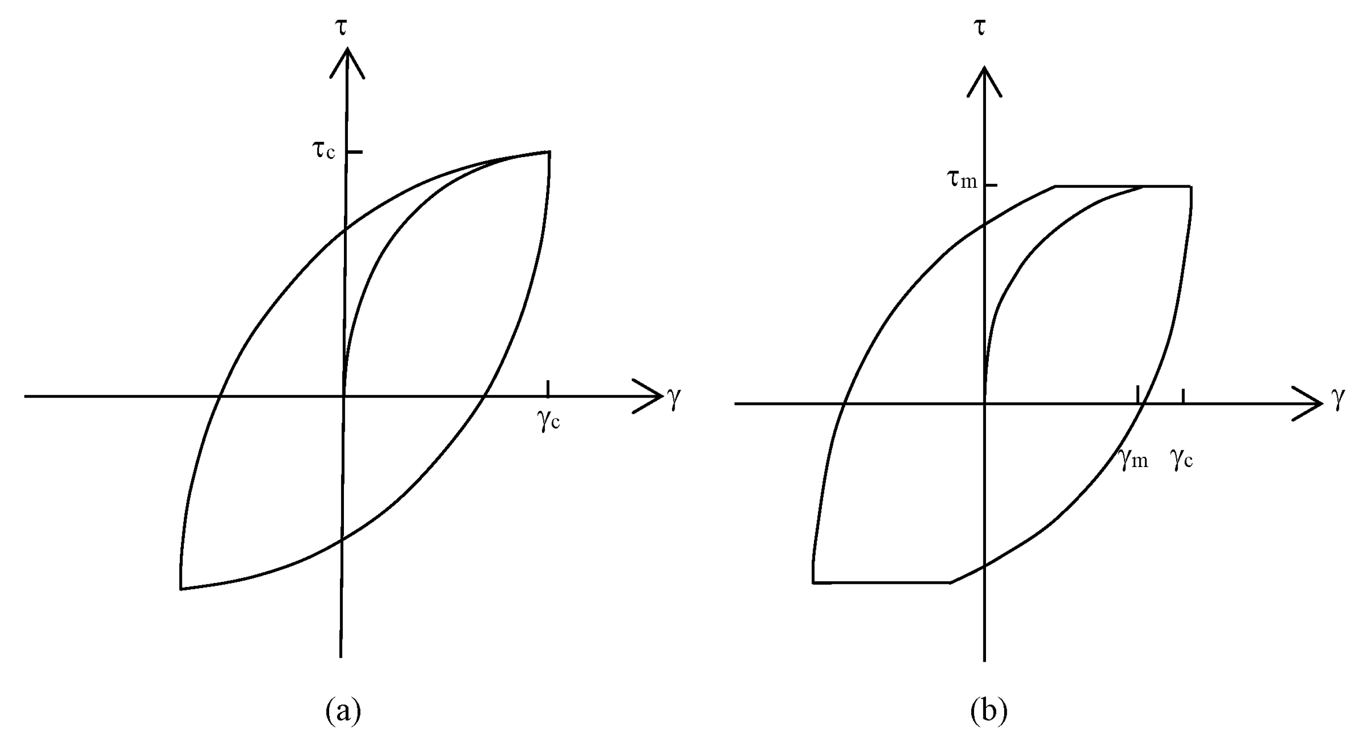
2.1. Soil Models

The first model is the hyperbolic model, where the modulus degradation curves govern the nonlinear soil behavior, and the ultimate strength is not defined explicitly. The reference strain concept defines the nonlinear soil behavior in the hyperbolic model. Figure 1a shows a loading–unloading–reloading cycle in the hyperbolic model. The second model is the Mohr–Coulomb (MC), in which the shear strength limits the ultimate stress that can be sustained. Figure 1b depicts a loading–unloading–reloading cycle in the MC model. Both models employ Masing’s rule for unloading/reloading behavior. However, the resulting damping ratio could be higher in the MC model, depending on the shear strain. According to Figure 1, the stress–strain behavior in MC for strains up to the yield strain γ_m is the same as in the hyperbolic model. However, the dissipated energy is greater in the MC when the accumulated shear strain is greater than the yield strain. Therefore, the models yield different damping values, particularly at shallow depths where the shear strength of cohesionless soils is significantly lower.

The definition of hysteretic damping is the ratio of the energy dissipated in one cycle to the maximum stored energy. The damping ratio for the stress–strain loops shown in Figure 1a can be calculated using Equation (1) in the hyperbolic model.

$${\mathrm{D}}_{\mathrm{masing}}=\frac{2}{\pi }\left\{2\frac{1+\frac{{\gamma }_c}{{\gamma }_{ref}}}{{\left(\frac{{\gamma }_c}{{\gamma }_{ref}}\right)}^2}\left[\frac{{\gamma }_c}{{\gamma }_{ref}}-\ln \left(1+\frac{{\gamma }_c}{{\gamma }_{ref}}\right)\right]-1\right\}$$

(1)

Equation (1) includes the γ_c, the shear strain due to the dynamic load, and γ_ref, the soil property defining the modulus degradation curves. In addition to the parameters used in the hyperbolic model (γ_c and γ_ref), the MC model includes the strain at which the maximum shear stress is sustained, γ_m. If the cyclic strain γ_c is less than the γ_m, the resulting damping ratio becomes equal to the one in the hyperbolic model. Once the strain γ_c is greater than γ_m in the MC model, the damping ratio formulation is as in Equation (2). Equations (1) and (2) were given in the FLAC^3D manual [32]. However, in this study, the denominator of the multiplication has been corrected to 1/(γ_c/γ_m).

$${\mathrm{D}}_{\mathrm{masing}}=\frac{2}{\pi }\left\{2\frac{1+\frac{{\gamma }_m}{{\gamma }_{ref}}}{{\left(\frac{{\gamma }_m}{{\gamma }_{ref}}\right)}^2}\left[\frac{{\gamma }_m}{{\gamma }_{ref}}-\ln \left(1+\frac{{\gamma }_m}{{\gamma }_{ref}}\right)\right]-1\right\}\frac{1}{\frac{{\gamma }_c}{{\gamma }_m}}+\frac{2}{\pi }\frac{\left({\gamma }_c-{\gamma }_m\right)}{{\gamma }_c}$$

(2)

In this study, the soil’s small strain shear moduli (G_max) were determined by Equations (3) and (4) (Seed and Idris [16]), and the bulk modulus is calculated by elastic theory using Poisson’s ratio. The maximum shear modulus computed using Equation (3) was applied to the soil domain considering the initial confining stresses. However, a minimum cut-off value of 10 kPa was applied to G_max to prevent the soil domain near the ground surface from having an unrealistically low initial soil modulus.

$$G_{max}=21.7 {(K_2)}_{max} p_a {\left(\frac{{{\sigma }^{\prime }}_m}{p_a}\right)}^{0.5}$$

(3)

$${(K_2)}_{max}=3.5 {\left(D_R\right)}^{2/3}$$

(4)

The nonlinear stress–strain behavior of soils can be considered by normalized shear modulus reduction (G/G_max) curves. Many researchers have studied the nonlinear behavior of cohesionless soils under cyclic loads, and reduction curves have been suggested [14,15,16]. The curves suggested by Seed and Idriss [16] have been implemented in the verification analyses presented by Boulanger et al. [11], Thavaraj et al. [33], and Kwon & Yoo [34]. In this study, effective stress-dependent curves of Darendeli [14] were employed to better consider the variation with depth (Figure 2a). The shear modulus reduction equation is given in Equation (5). The reference strain in the equation depends on the effective confining stress as in Equation (6), according to Darendeli [14]. The hysteretic damping command in FLAC^3D [32] was utilized for the soil domain in the model. The reference strain values were assigned to each zone by considering the initial effective stress (total stress approach). However, the maximum shear strain was on the order of 0.1–0.3% in the study performed by Darendeli [14], which could not involve the large strain (>1%) behavior. In contrast, the study of Seed and Idriss [16] showed that the G/G_max value for modulus degradation curves at 3% shear strain varies between 0.03 and 0.05. Therefore, a cut-off for G/G_max is required to accurately represent the large strain behavior in the modulus degradation. Since the experimental study presented by Darendeli (2001) does not include the large strain data (≥1%), 0.05 was assumed for minimum G/G_max considering the Seed and Idriss [16] curves. The minimum cut-off value of 0.05 was applied for the modulus reduction ratio to prevent further increase in damping beyond a certain shear strain. The damping ratio variation with shear strain curves in the hyperbolic model is shown in Figure 2b.

$$\frac{G}{G_{max}}=\frac{1}{1+{\left(\frac{\gamma }{{\gamma }_{ref}}\right)}^{0.919}}$$

(5)

$${\gamma }_r=0.0352{\left[\frac{{{\sigma }^{\prime }}_m}{p_a}\right]}^{0.3483}$$

(6)

It should be noted that the damping values in Figure 2b are calculated using Equation (1), which obeys Masing’s [35] criterion for unloading/reloading. However, the MC model approach yields different damping ratio values than the hyperbolic model. Equations (1) and (2) can be used to compare the damping ratios at various cyclic strains for a given confining stress. Figure 3 shows the damping ratio variation with shear strain for hyperbolic and MC models for the given confining stress levels. According to the figure, the damping at relatively higher strains is significantly greater in the MC model, especially at the lower confining stresses. Consequently, a perfectly plastic MC model could cause the damping to be considerably higher than the hyperbolic model.

2.2. Verification Analyses Using Hyperbolic and MC Constitutive Models

In this study, two centrifuge tests published in the literature were used for verification purposes. Figure 4 shows the test containers (Gohl [30] and Wilson [31]) in the prototype units. In Gohl [30], a pile with a diameter of 0.57 m was placed inside dry Nevada sand with a relative density of D_R = 40%. The single mass was placed on top of the pile extending to 2.0 m from the ground surface.

The diameter and the length of the highly instrumented single pile in Wilson [31] were 0.67 m and 16.7 m, respectively. A 49 Mg mass on the pile created a single degree of freedom system. The free height of the single pile was 3.8 m. The soil in which the piles were embedded was the saturated Nevada sand placed at two different relative densities. The thicknesses of these layers were 9.4 m and 11.3 m, and the relative densities were 55% and 80%, respectively.

The damping ratio formulations given in Equations (1) and (2) depend on the reference strain (γ_ref) and yield strain (γ_m), where the last of which depends on the shear strength. The friction angles for medium-dense and dense sand were selected as 36° and 40° for soil layers in Wilson (1998). The friction angle was assumed to be 34° for the sand in Gohl (1991). The soil parameters selected for the verification analyses are given in

Table 1. The soil parameters selected for the verification analyses.

	Wilson, 1998		Gohl, 1991
Layer	Layer 1	Layer 2	Single Layer
Effective unit weight, γ′ (kN/m3)	9.5	9.9	15.1
Relative density (%)	55	80	40
Friction angle, φ′ (°)	36	40	34
Dilation angle ψ (°)	4	8	2
Poisson’s ratio, ν	0.45	0.45	0.30

.

In this study, the numerical model was created in FLAC^3D [32]. The model dimensions in x-y-z directions are 16 m × 10 m × 12 m and 20 m × 51 m × 20 m in Gohl [30] and Wilson [31], respectively. The zone sizes must be fine enough to accurately transmit the waves from the base into the model. Finer zones are used in the vicinity of the pile in the lateral direction, and the zone sizes gradually increase using an aspect ratio of 1.1. In the vertical direction, the dimension of each solid zone is constant. Still, the height of each element must be lower than the limit suggested by Kuhlemeyer and Lysmer [36], which (Δl) is one-tenth of the wavelength (λ) of the input wave motion (Δl < λ/10). The minimum zone size in the vertical direction is selected (Δl < λ/10 = 1.0 m). The bottom boundary of the model was fixed, and the dynamic free-field boundaries were applied to the sides. Due to symmetry, half of the model is presented in Figure 5.

Although the piles and the structure are three-dimensional in nature, they were modeled with the beam elements for simplicity. The structural elements (beam) were rigidly connected to the surrounding soil, where the pile displacement is the same as the deformation of the soil. The rigid connection approach was adopted by several researchers [12,13,37]. Since the problem is a laterally loaded pile model under dynamic loading, the key property affecting the response is the flexural stiffness of the pile and the superstructure. The superstructure properties summarized in

Table 2. The superstructure properties in the verification analyses.

Structure (Wilson, 1998)				Structure (Gohl, 1991)
Flexural Stiffness EI (MN·m2)	Height (m)	Mass (Mg)	Tfixed (s)	Flexural Stiffness EI (MN·m2)	Height (m)	Mass (Mg)	Tfixed (s)
427	3.8	49	0.3	172	2.0	52.2	0.3

were assigned to the beam elements used in the numerical analyses.

The numerical models for verification analyses were created in the FLAC^3D and analyzed under the same input motions as in the centrifuge tests. Gohl [30] applied a random input motion having 0.15 g acceleration amplitude to the rigid container base. The acceleration–time history of the motion is given in Figure 6 (provided by Amin Rahmani and Mahdi Taibeat). In Wilson [31], two real earthquake records (Loma Prieta, 1989-Santa Cruz station and Kobe, 1995-Port Island station) were used in the centrifuge tests. The UC Davis centrifuge laboratory provides the input motion’s acceleration time history. Although the soil in Wilson [31] was saturated sand, the Santa Cruz motion with a_max = 0.05 g (Event K) did not cause significant excess pore water pressure. Hence, the event was selected in this study for the non-liquefiable case. Event I and Event J are the motions of Santa Cruz and Kobe with a_max = 0.49 g and a_max = 0.22 g, respectively, in which the medium dense sand completely liquefied under these events in Wilson [31].

2.3. Numerical Analyses Using Hyperbolic and MC Constitutive Models

A new single pile–soil–structure model was created and analyzed using the additional earthquake records in this study. The numerical model consists of a single layer of dry cohesionless soil where D_R = 55%. The unit weight of the soil was 18 kN/m³. The friction angle and dilation angle values were 36° and 4°, respectively. The model dimensions were 20 × 20 × 30 in x, y, and z directions. The soil properties used in the verification analyses are given in

Table 3. The soil properties used in the numerical analyses.

Layer	Single Layer
Effective unit weight, γ′ (kN/m3)	18
Relative density (%)	55
Friction angle, φ′ (°)	36
Dilation angle ψ (°)	4
Poisson’s ratio, ν	0.30

. The bottom boundary of the model was fixed, and the lateral boundaries were free-field to prevent wave reflection from the model sides to the model.

The diameter of the single pile was 0.65 m in the analyses, and the elastic modulus of concrete (E = 30 GPa) was set to the pile. The pile length was 12 m, setting the slenderness ratio L/D = 18 (flexible pile). A single degree of freedom system was created with a column having the same properties as the pile. A single 40-tonne mass was placed at the top of the 5 m high column. The fixed base natural period of the single degree of freedom system was approximately 0.5 s. The parameters for the pile and the structure used in the numerical analyses are given in

Table 4. Pile and superstructure properties used in the numerical analyses.

Pile		Structure
Diameter (m)	Length (m)	E (MN/m2)	I (m4)	Mass (Mg)	Flexural Stiffness EI (MN·m2)	H (m)	Tfixed (s)
0.65	16	30,000	0.00876	40	262.8	5.0	0.5

.

The earthquake records were selected from the PEER database [38], with corresponding parameters given in

Table 5. The earthquake records used in the soil–pile–structure interaction analyses.

PEER Code	Earthquake	Year	Mw	Station	Fault	Rrup (km)	(Vs)30 (m/s)	Pga (g)	SF
RSN143	Tabas, Iran	1978	7.35	Tabas	Reverse	2.05	766	0.14	0.17
RSN285	Irpinia, Italy-01	1980	6.90	Bagnoli Irpinio	Normal	8.18	650	0.13	1.0
RSN572	Taiwan SMART1 (45)	1986	7.30	SMART1 E02	Reverse	51.35	672	0.14	1.0
RSN1091	Northridge-01	1994	6.69	Vasquez Rocks Park	Reverse	23.64	996	0.15	1.0
RSN1206	Chi-Chi, Taiwan	1992	7.62	CHY042	Reverse Oblique	28.17	665	0.15	1.5
RSN1613	Duzce, Turkey	1999	7.14	Lamont 1060	Strike Slip	25.88	782	0.16	3.0

. The stations where the average shear wave velocity (V_s,30) values were a minimum of 650 m/s (almost bedrock motion) were selected so that the input motions could be directly applied to the bottom of the model. The original records were linearly scaled by the given factors (SF) such that the peak ground accelerations were obtained around 0.15 g without changing the frequency content. The acceleration time histories of the selected motions are shown in Figure 7.

3. Analysis Results

3.1. Verification Analysis

The soil–pile–structure systems created for the verification analyses were subjected to base excitation with the earthquake input motions in Figure 6. The results of the acceleration response spectrum of the structure and the maximum bending moments that occurred along the pile are presented. This study classified the verification analyses as Case 1 and Case 2 for non-liquefiable and liquefiable soils, respectively.

3.1.1. Non-Liquefiable Soil (Case 1)

The structure responses in Case 1 (Gohl, 1991 [30] and Event K in Wilson, 1998 [31]) were compared with the centrifuge test results through the acceleration response spectra (ARS), as shown in Figure 8. The MC model results were close to the test results in Gohl for both the peak and the spectral accelerations, whereas the hyperbolic model slightly overestimates the accelerations (Figure 8a). The hyperbolic and MC models slightly overestimate the spectral accelerations in the high-frequency domain and underestimate the low-frequency domain under Event K as shown in Figure 8b.

The model responses were compared through the maximum bending moments along the pile. Figure 9a shows the results of the study by Gohl [30], where the bending moments were captured by MC and were overestimated by the hyperbolic model. The bending moments obtained using both MC and hyperbolic models agreed with the centrifuge test results in Event K (Wilson, [31]).

The results showed that the hyperbolic and MC models could be used to simulate the soil behavior by applying a cut-off value of 0.05 to the G/G_max value. It should be noted that the assigned cut-off allows limiting the damping ratio. When the cut-off value was set to 0.02, the hyperbolic model yielded closer results than the MC model. Therefore, a 0.05 value was recommended for the G/G_max in the MC model to get more accurate responses.

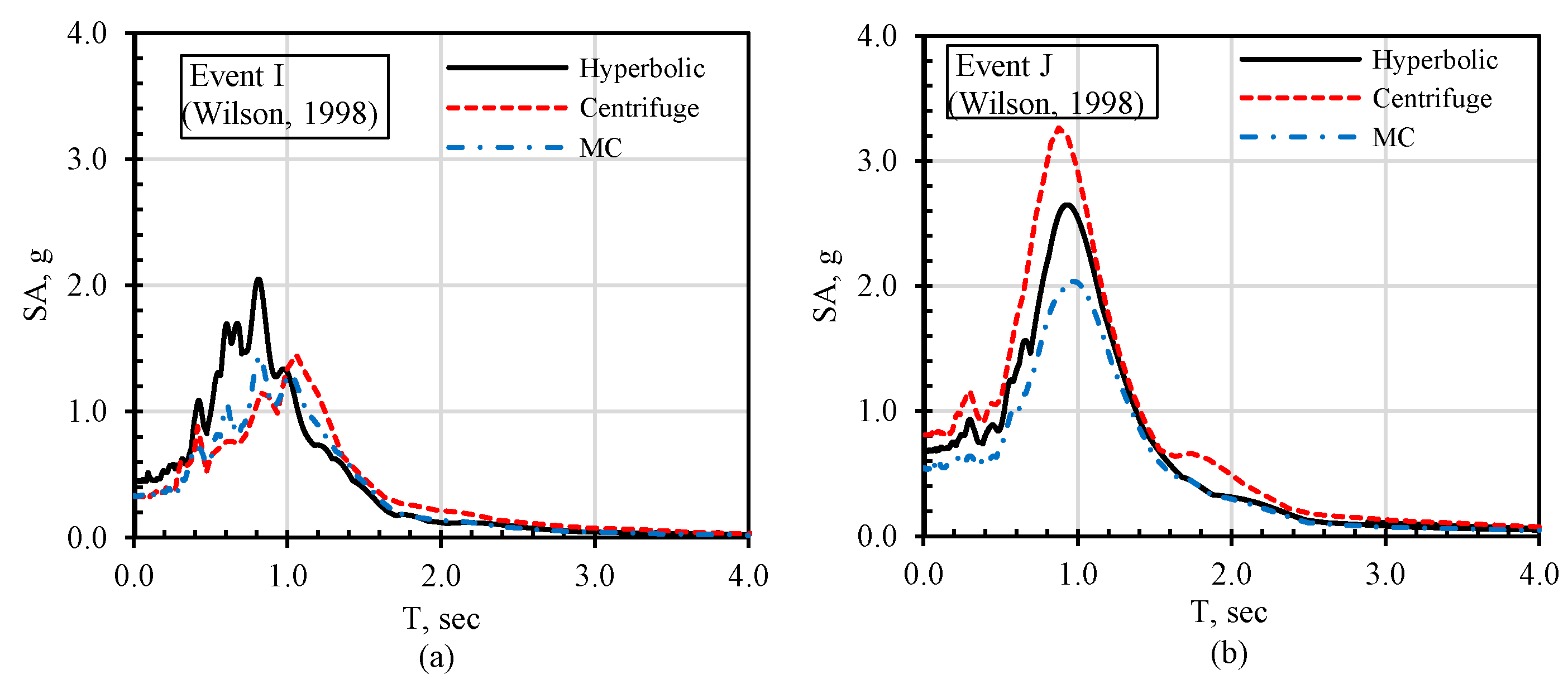
3.1.2. Liquefiable Soil (Case 2)

The soil–pile–structure system response in the liquefiable soils under Event I and Event J (Case 2) were investigated by comparing the analysis results with the centrifuge test outputs. Figure 10a shows the acceleration response spectra for Event I, where the hyperbolic model slightly overestimates the response while the MC model better captures the general trend. However, the MC model significantly underestimates the accelerations in Event J (Figure 10b), in which the hyperbolic model yields closer results. The reason for the high superstructure response in the centrifuge test under Event J has been reported as the reduction in the pore pressures, which result in increased effective stresses (Boulanger, [11], and reduced damping. Since the pore water pressures were not considered in the models employed in this study, the analysis results were overdamped compared to the centrifuge results. The spectral accelerations obtained through the hyperbolic model were closer to the centrifuge test results since the hyperbolic model provides lower damping.

The model responses in the liquefiable soil case were compared through the maximum bending moments along the pile. Figure 11a compares Event I, where the bending moments were closer in the MC model, to the centrifuge test results. In contrast, the hyperbolic model slightly overestimated the bending moments at the shallow depths and underestimated the depths greater than 3 m. Figure 11b shows the pile response under Event J. Both models underestimated the bending moments for shallow depths due to the low superstructure accelerations. However, the hyperbolic model led to a closer pile response in Event J than the MC model. Overall, the MC model caused higher damping than the hyperbolic model due to the perfectly plastic behavior, especially under high-intensity motions. Accordingly, the resulting pile and structure responses were lower in the MC than in the hyperbolic model.

In general, differences in the spectral accelerations and bending moments were observed the verification analysis. Similar inconsistencies were observed in past studies that have used the same centrifuge tests for verification purposes [12,33,34,37]. The primary reason might be the uncertainties in soil behavior. The complex nature of centrifuge tests, and sequential loading that might change the relative density of soil after each test, could be the secondary effect of the uncertainties that could not be taken into consideration in the numerical analyses. Therefore, the verification analysis results were assumed to be promising, considering the complex nature of the problem.

3.2. Numerical Analyses

Further numerical analyses were performed with the earthquake records given in Table 1 to reveal the effect of hysteretic soil damping more clearly. The superstructure accelerations, acceleration response spectra, and maximum bending moments along the pile were compared for the Hyperbolic and MC models.

The numerical analysis results are presented for low-intensity and high-intensity response outputs. Figure 12 shows the acceleration time history of the superstructure, which consists of the first set of earthquake events: RSN143, RSN572, and RSN1614, where the peak structure acceleration (PA) values vary between 0.15 g and 0.31 g. The acceleration response spectra of the structure for the events are compared in Figure 13 with the ARS of the input motions (IM). According to the ARS results, the natural period of the single degree of freedom system is approximately 1 s, where the spectral accelerations reach the peak value. Peak spectral accelerations (PSA) vary from 0.94 g to 1.43 g in the hyperbolic model and between 0.62 g and 1.02 g for the MC model. Figure 14 shows the variation of the maximum bending moments with depth for the first set of earthquakes. The hyperbolic model results in 27%, 55%, and 63% higher bending moments than the MC model for RSN143, RSN572, and RSN1613, respectively. According to the analysis results, the structure and pile responses were greater in the hyperbolic model than in the MC for all the first set of earthquake records.

Figure 15 shows the acceleration time histories of the superstructure for the second set of earthquakes, which consists of RSN285, RSN1091, and RSN1206, where the PA values vary between 0.24 g and 0.70 g. The acceleration response spectra of the structure for the second set of earthquakes were compared in Figure 16 with the ARS of the input motions (IM). According to the ARS results, the natural period of the single degree of freedom system is slightly higher than 1 s, where the spectral accelerations reach the peak value. Peak spectral accelerations varied from 1.73 g to 3.69 g in the hyperbolic model and between 0.94 g and 2.32 g for the MC model. Figure 17 shows the variation of the maximum bending moments with depth for the second set of earthquakes. The hyperbolic model results in 38%, 45%, and 49% higher bending moments than the MC model for RSN285, RSN1091, and RSN1206, respectively. Again, the structure responses were greater in the hyperbolic model than in the MC for all the second set of earthquake records.

The results obtained from the soil–pile–structure interaction analyses have shown the effect of soil damping on the system response. Moreover, it was revealed that the selection of earthquake records plays a key role in the outputs. Although the peak ground accelerations of the input motions were close, the resulting superstructure accelerations were significantly different, depending on the frequency content.

The peak structure acceleration (PA), the peak spectral acceleration (PSA), and maximum bending moments that occurred under the given earthquakes were summarized in

Table 6. Summary of the numerical analysis results under various earthquakes.

	RSN	143	572	1613	285	1091	1206
PA (g)	Hyperbolic MC	0.24	0.31	0.24	0.53	0.37	0.70
		0.18	0.19	0.15	0.33	0.24	0.41
PSA (g)	Hyperbolic MC	1.27	1.43	0.94	2.87	1.73	3.69
		0.95	1.02	0.62	1.79	0.94	2.32
Mmax (kN·m)	Hyperbolic MC	533	701	543	1180	862	1580
		419	451	333	853	593	1060

for both hyperbolic and MC models for comparison. Overall, the superstructure accelerations in the hyperbolic model were higher than in the MC model for all the selected earthquake records. Accordingly, the bending moments were greater again in the hyperbolic model. To summarize, the results of dynamic soil–pile–structure interaction analyses are highly influenced by the input motion and modeling approaches, such as the selection of the constitutive model.

4. Conclusions

The aim of this study is to investigate the influence of hysteretic soil damping on the pile and structure response in the dynamic soil–pile–structure analyses. For this purpose, two well-known centrifuge tests were simulated and analyzed in FLAC^3D for verification using two constitutive soil models. Further analyses were performed with the additional earthquake records in a single pile–soil–structure system. The conclusions from the fully nonlinear analyses are outlined below:

• The nonlinear soil behavior can be modeled using the modulus degradation curves in numerical analyses of soil–pile–structure problems. According to the verification analyses, if the soil damping is integrated into the model accurately, the use of modulus degradation can represent the response even for liquefiable soils.
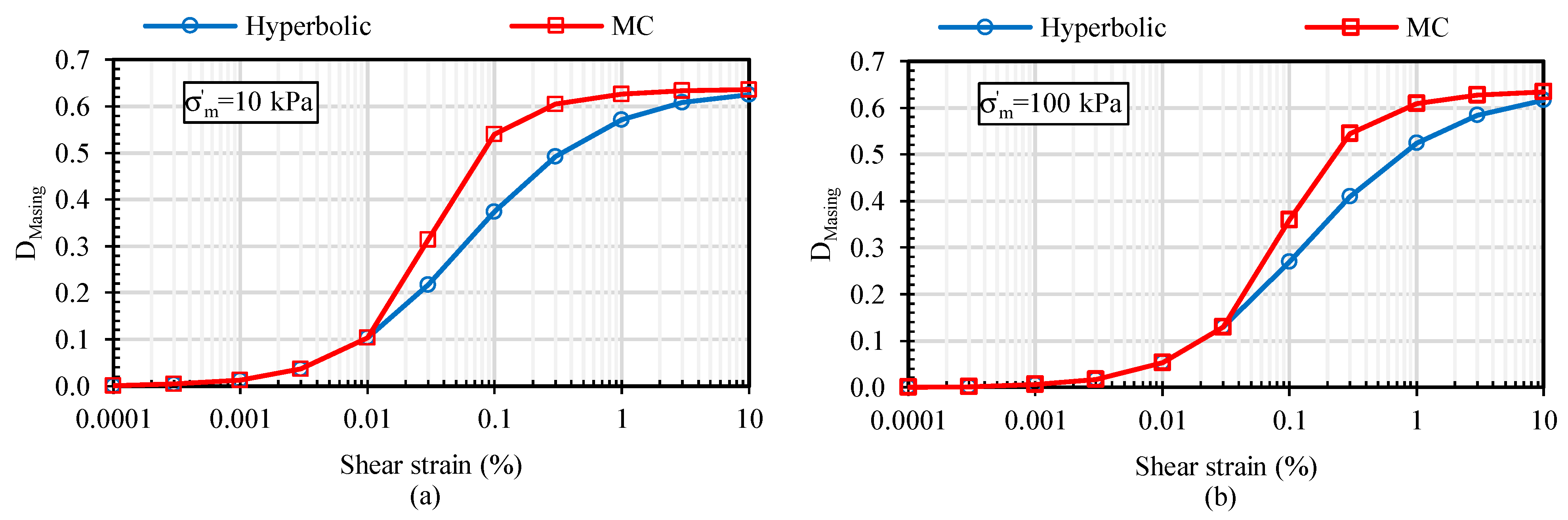
• The constitutive models without a cut-off for G/G_max might cause significantly higher damping ratios. To overcome the higher damping ratio problem, the minimum G/G_max value was set to 0.05, and closer results were obtained in the verification analyses. Thus, the cut-off must be applied to eliminate higher damping ratios at large strains. Generally, the agreement between the 3D analysis results and centrifuge test outputs was reasonably good.
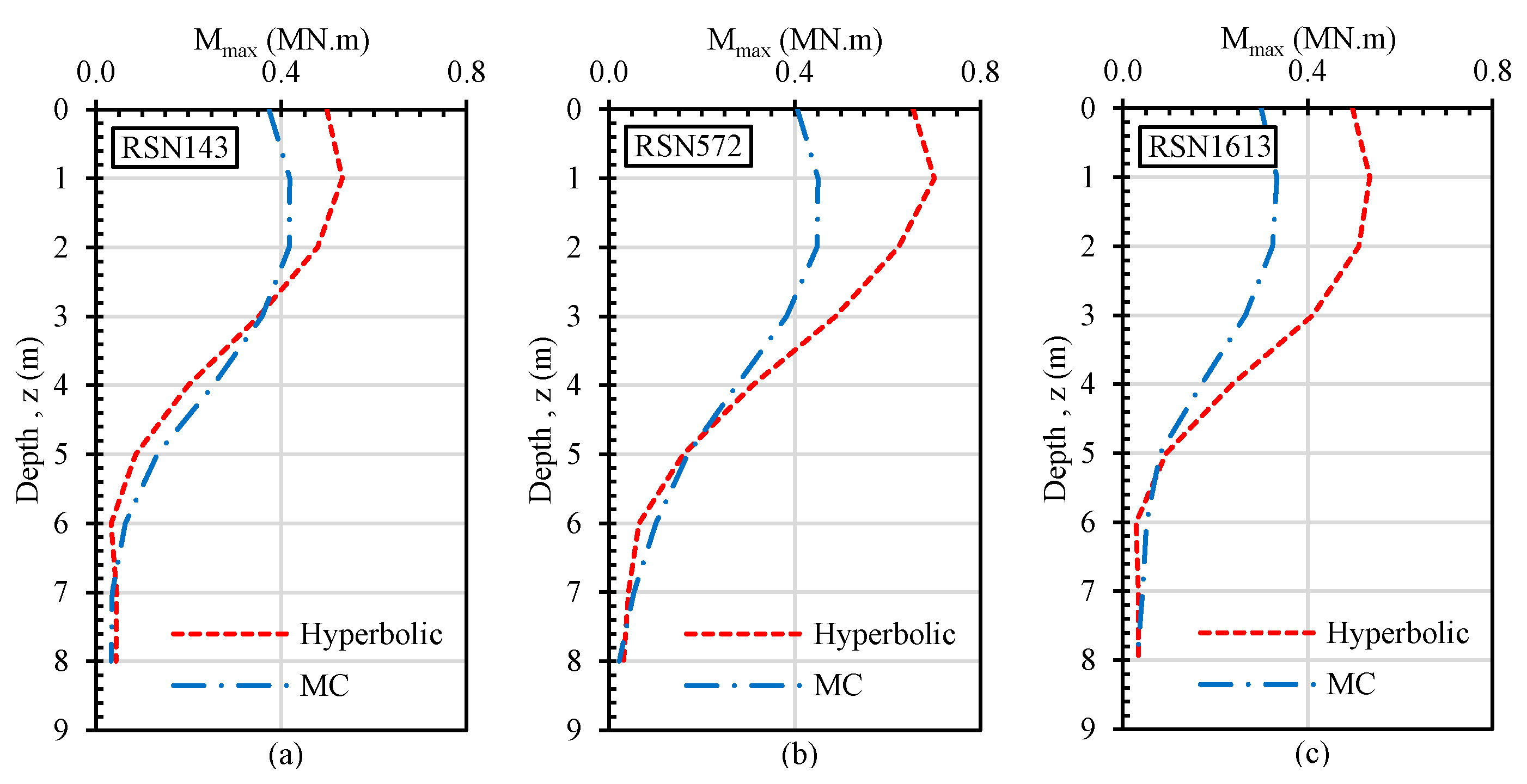
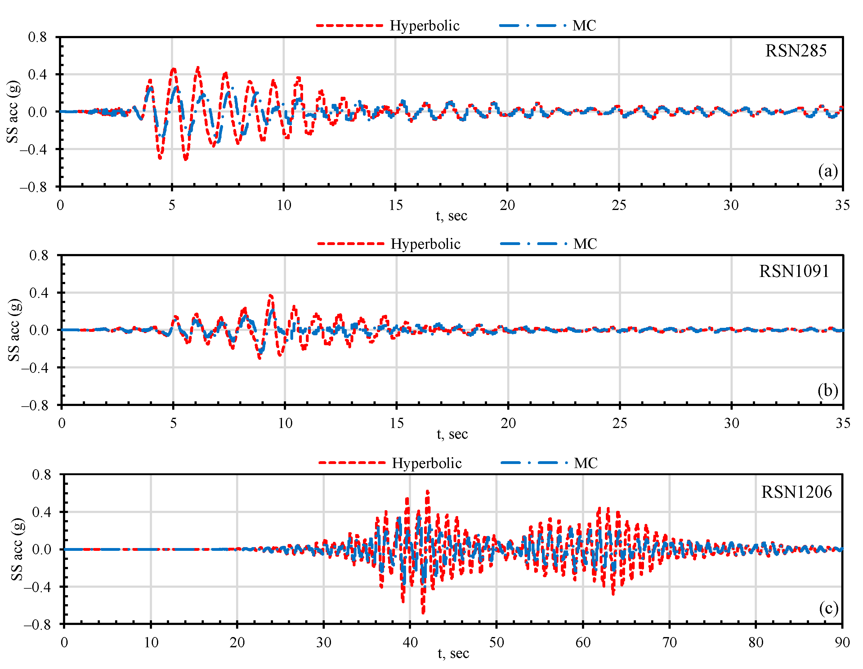
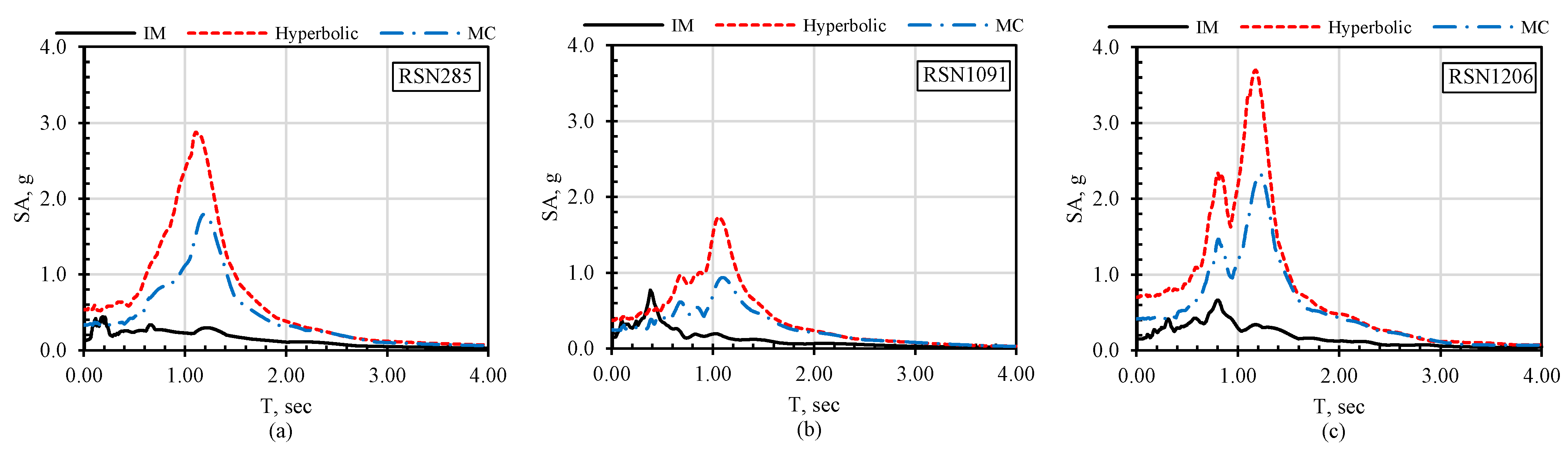
• Dynamic single pile–soil–structure analyses performed with the additional earthquake records selected from the PEER database have confirmed the effect of soil damping on the pile and structure response. Peak structure accelerations, peak spectral accelerations, and bending moments along the pile were compared for hyperbolic and MC models. The peak structure accelerations and the peak bending moments for all earthquake records were greater in the hyperbolic model. The difference between the hyperbolic and MC models varies between 27 and 63%, depending on the applied earthquake record. The results have indicated that the soil damping ratio in the MC model could be considerably high, especially in the shallow depths, since the lower confining stresses cause the shear strength to be significantly low.
• Apart from the damping effect, the analyses have shown that the selection of earthquake records significantly affects the structure and pile response. In particular, although the selected earthquakes have the same peak ground acceleration, as much as three times the difference might occur in the resulting structure accelerations (RSN 1613 and RSN 1206).

The results have indicated that the damping ratio affects the soil–pile–structure response significantly; hence the selection of the constitutive soil model, which represents the damping characteristics of the soil–pile–structure system, is critical. In this study, the soil–pile–interaction problem was investigated through the single pile; however, group pile behavior should be examined in future studies to better understand the actual problem.

References

- Brown, D.A.; Shie, C.-F. Some numerical experiments with a three dimensional finite element model of a laterally loaded pile. Comput. Geotech. 1991, 12, 149–162. [Google Scholar] [CrossRef]
- Luo, C.; Yang, X.; Zhan, C.; Jin, X.; Ding, Z. Nonlinear 3D finite element analysis of soil–pile–structure interaction system subjected to horizontal earthquake excitation. Soil Dyn. Earthq. Eng. 2016, 84, 145–156. [Google Scholar] [CrossRef]
- Giannakos, S.; Gerolymos, N.; Gazetas, G. Cyclic lateral response of piles in dry sand: Finite element modeling and validation. Comput. Geotech. 2012, 44, 116–131. [Google Scholar] [CrossRef]
- Bathe, K.-J. Finite Element Procedures; Klaus-Jurgen Bathe: Watertown, MA, USA, 2006. [Google Scholar]
- Wang, S.; Kutter, B.L.; Chacko, M.J.; Wilson, D.W.; Boulanger, R.W.; Abghari, A. Nonlinear seismic soil-pile structure interaction. Earthq. Spectra 1998, 14, 377–396. [Google Scholar] [CrossRef]
- Nogami, T.; Otani, J.; Konagai, K.; Chen, H.-L. Nonlinear soil-pile interaction model for dynamic lateral motion. J. Geotech. Eng. 1992, 118, 89–106. [Google Scholar] [CrossRef]
- Allotey, N.; El Naggar, M.H. A numerical study into lateral cyclic nonlinear soil–pile response. Can. Geotech. J. 2008, 45, 1268–1281. [Google Scholar] [CrossRef]
- Poulos, H.G. Behavior of laterally loaded piles: I-single piles. J. Soil Mech. Found. Div. 1971, 97, 711–731. [Google Scholar] [CrossRef]
- Banerjee, P.; Davies, T. The behaviour of axially and laterally loaded single piles embedded in nonhomogeneous soils. Geotechnique 1978, 28, 309–326. [Google Scholar] [CrossRef]
- Randolph, M.F. The response of flexible piles to lateral loading. Geotechnique 1981, 31, 247–259. [Google Scholar] [CrossRef]
- Boulanger, R.W.; Curras, C.J.; Kutter, B.L.; Wilson, D.W.; Abghari, A. Seismic soil-pile-structure interaction experiments and analyses. J. Geotech. Geoenviron. Eng. 1999, 125, 750–759. [Google Scholar] [CrossRef]
- Finn, W. A study of piles during earthquakes: Issues of design and analysis. Bull. Earthq. Eng. 2005, 3, 141–234. [Google Scholar] [CrossRef]
- Rahmani, A.; Taiebat, M.; Finn, W.L.; Ventura, C.E. Evaluation of p-y springs for nonlinear static and seismic soil-pile interaction analysis under lateral loading. Soil Dyn. Earthq. Eng. 2018, 115, 438–447. [Google Scholar] [CrossRef]
- Darendeli, M.B. Development of a New Family of Normalized Modulus Reduction and Material Damping Curves; The University of Texas at Austin: Austin, TX, USA, 2001. [Google Scholar]
- Ishibashi, I.; Zhang, X. Unified dynamic shear moduli and damping ratios of sand and clay. Soils Found. 1993, 33, 182–191. [Google Scholar] [CrossRef]
- Seed, H.B.; Idriss, I.M. Soil Moduli and Damping Factors for Dynamic Response Analysis; EERC: Grand Forks, ND, USA, 1970. [Google Scholar]
- Matasović, N.; Vucetic, M. Cyclic characterization of liquefiable sands. J. Geotech. Eng. 1993, 119, 1805–1822. [Google Scholar] [CrossRef]
- Vucetic, M.; Dobry, R. Effect of soil plasticity on cyclic response. J. Geotech. Eng. 1991, 117, 89–107. [Google Scholar] [CrossRef]
- Schnabel, P.; Seed, H.B.; Lysmer, J. Modification of seismograph records for effects of local soil conditions. Bull. Seismol. Soc. Am. 1972, 62, 1649–1664. [Google Scholar] [CrossRef]
- Groholski, D.R.; Hashash, Y.M.; Kim, B.; Musgrove, M.; Harmon, J.; Stewart, J.P. Simplified model for small-strain nonlinearity and strength in 1D seismic site response analysis. J. Geotech. Geoenviron. Eng. 2016, 142, 04016042. [Google Scholar] [CrossRef]
- Phillips, C.; Hashash, Y.M. Damping formulation for nonlinear 1D site response analyses. Soil Dyn. Earthq. Eng. 2009, 29, 1143–1158. [Google Scholar] [CrossRef]
- Park, D.; Hashash, Y.M. Soil damping formulation in nonlinear time domain site response analysis. J. Earthq. Eng. 2004, 8, 249–274. [Google Scholar] [CrossRef]
- Régnier, J.; Bonilla, L.F.; Bard, P.Y.; Bertrand, E.; Hollender, F.; Kawase, H.; Sicilia, D.; Arduino, P.; Amorosi, A.; Asimaki, D.; et al. PRENOLIN: International Benchmark on 1D Nonlinear Site-Response Analysis—Validation Phase Exercise. Bull. Seismol. Soc. Am. 2018, 108, 876–900. [Google Scholar] [CrossRef]
- Beaty, M.H.; Byrne, P.M. UBCSAND Constitutive Model, Version 904aR; Itasca UDM: Minneapolis, MN, USA, 2011; p. 69. [Google Scholar]
- Boulanger, R.; Ziotopoulou, K. PM4Sand (Version 3): A Sand Plasticity Model for Earthquake Engineering Applications. In Center for Geotechnical Modeling Report No. UCD/CGM-15/01; Department of Civil and Environmental Engineering, University of California: Davis, CA, USA, 2015. [Google Scholar]
- Cheng, Z. Application of SANISAND Dafalias-Manzari model in FLAC 3D. In Continuum and Distinct Element Numerical Modeling in Geomechanics, (October 2013); Itasca International Inc.: Minneapolis, MN, USA, 2013. [Google Scholar]
- Hokmabadi, A.S.; Fatahi, B.; Samali, B. Assessment of soil–pile–structure interaction influencing seismic response of mid-rise buildings sitting on floating pile foundations. Comput. Geotech. 2014, 55, 172–186. [Google Scholar] [CrossRef]
- Maheshwari, B.K.; Truman, K.; El Naggar, M.; Gould, P. Three-dimensional nonlinear analysis for seismic soil–pile-structure interaction. Soil Dyn. Earthq. Eng. 2004, 24, 343–356. [Google Scholar] [CrossRef]
- Guin, J.; Banerjee, P. Coupled soil-pile-structure interaction analysis under seismic excitation. J. Struct. Eng. 1998, 124, 434–444. [Google Scholar] [CrossRef]
- Gohl, W.B. Response of Pile Foundations to Simulated Earthquake Loading: Experimental and Analytical Results Volume I. Ph.D. Thesis, University of British Columbia, Vancouver, BC, Canada, 1991. [Google Scholar]
- Wilson, D.W. Soil-Pile-Superstructure Interaction in Liquefying Sand and Soft Clay; Citeseer: University Park, PA, USA, 1998; Volume 1998. [Google Scholar]
- Itasca Consulting Group, Inc. FLAC3D—Fast Lagrangian Analysis of Continua in Three-Dimensions, Version 7.0; Itasca: Minneapolis, MN, USA, 2019. [Google Scholar]
- Thavaraj, T.; Liam Finn, W.; Wu, G. Seismic response analysis of pile foundations. Geotech. Geol. Eng. 2010, 28, 275–286. [Google Scholar] [CrossRef]
- Kwon, S.Y.; Yoo, M. Study on the dynamic soil-pile-structure interactive behavior in liquefiable sand by 3D numerical simulation. Appl. Sci. 2020, 10, 2723. [Google Scholar] [CrossRef]
- Masing, G. Eigenspannungen und Verfestigung beim Messing [Fundamental Stresses and Strengthening with Brass]; International Congress of Applied Mechanich: Zurich, Switzerland, 1926. [Google Scholar]
- Kuhlemeyer, R.L.; Lysmer, J. Finite element method accuracy for wave propagation problems. J. Soil Mech. Found. Div. 1973, 99, 421–427. [Google Scholar] [CrossRef]
- Finn, W.; Fujita, N. Piles in liquefiable soils: Seismic analysis and design issues. Soil Dyn. Earthq. Eng. 2002, 22, 731–742. [Google Scholar] [CrossRef]
- The Pacific Earthquake Engineering Research Center (PEER). PEER Strong Motion Database on Line. Available online: https://peer.berkeley.edu/peer-strong-ground-motion-databases (accessed on 5 April 2022).