Adaptive Industrial Control System Attack Sample Expansion Algorithm Based on Generative Adversarial Network

Abstract

The scarcity of attack samples is the bottleneck problem of anomaly detection of underlying business data in the industrial control system. Predecessors have done a lot of research on temporal data generation, but most of them are not suitable for industrial control attack sample generation. The change patterns of the characteristics of the underlying business data attack samples can be divided into three types: oscillation type, step type, and pulse type. This paper proposes an adaptive industrial control attack sample expansion algorithm based on GAN, which expands the three types of features in different ways. The basic network structure of data expansion adopts GAN. According to the characteristics of oscillation type changes, momentum is selected as the optimizer. Aiming at the characteristics of step type changes, the Adam optimization method is improved. For pulse type features, attack samples are generated according to the location and length of the pulse. Compared with previous time-series data generation methods, this method is more targeted for each feature and has higher similarities.

1. Introduction

In recent years, security incidents occur frequently in industrial control systems. The traditional security research is mainly based on a firewall and trap system in the industrial control system. Once the defense system is broken, the intruder directly enters the business layer to tamper with business data, which will cause huge losses [1]. No matter how the attack is carried out, it will eventually lead to abnormal operation data at the bottom of the industrial control system and cause safety accidents. Anomaly detection of industrial underlying operating data is mainly used to identify runtime data anomalies, which is the last line of defense for security [2].

At present, a large amount of operation data has been accumulated in the industrial control system. However, most of these data are samples under normal conditions, with few abnormal samples, and none of them is the sample of the system being attacked. In order to study the underlying business data of industrial control system for anomaly detection, the research group collected 30 public industrial control datasets, and found that only two of them included the underlying data attack samples. They are the natural gas pipeline dataset [3] of the SCADA Laboratory of Mississippi State University (the gas dataset) and the Singapore dataset [4,5,6]. Due to the lack of attack samples, it is difficult to build more industrial control security datasets. Although some attack samples can be obtained from simulated attacks, they are not enough to support deep learning model training. It is an urgent problem to design an efficient data enhancement method for the characteristics of underlying business data.

At present, artificial intelligence deep learning algorithms are widely used in various fields. For example, convolutional neural networks are commonly used in target tracking and target detection [7,8]. In the field of data expansion, the most efficient and common way is GAN (Generative Adversarial Network) [9], but most GAN derivative networks do not apply to industrial control underlying business data attack samples. In 2019, Zhu et al. [10] and others proposed the time series data generation model of Bilstm-CNN GAN and published papers on nature. This method is mainly aimed at the time series data generation of ECG samples. ECG data have the characteristics of time sequence, periodicity and low data dimension. However, the step-type and pulse-type data in the underlying business data of industrial control are non-periodic, and the data dimension of the entire dataset is high, and there are many types of data changes. If BiLSTM-CNN GAN or other GANs for temporal data generation are used, step-type and pulse-type data will be treated as noise, and it is difficult to learn attack characteristics.

In order to solve the problems of the variety and non-periodicity of the attack sample characteristics of the industrial control system, this paper adopts different methods for different types of data. For oscillation type data, momentum is selected as the optimizer of its discriminator, and GAN is used to generate data directly. For Step type data, an improved Adam optimizer based on GAN is used. When the discriminator encounters step jump, the Adam optimizer decouples instantaneously to prevent step jump from being ignored as noise. For the pulse data, GAN is used to generate data for its positive samples. Then, the pulse signal is generated and inserted into the generated positive example sample. Finally, attack samples are formed.

The structure of the paper is as follows: The first section introduces the current situation of the scarcity of abnormal data in the industrial control system; the second section takes three data sets as examples to illustrate the characteristics of attack samples in industrial control system; the third section describes the current research status of the sequential sample generation algorithm and the commonly used optimizers; the fourth section is the specific principle and implementation process of the algorithm in this paper; the fifth section verifies the effectiveness of our algorithm and compares it with other algorithms; and the sixth section presents conclusions.

2. Background

The research object of anomaly detection technology for underlying business data in an industrial control system is the attacked business data. If there is no sufficient attack sample, all the deep learning anomaly detection algorithms for the underlying business data of industrial control will not be able to train. Three datasets are currently collected that contain samples of underlying business data attacks: the natural gas pipeline dataset of SCADA laboratory of Mississippi State University (the gas dataset), the Singapore dataset, and the real underlying business dataset of an oil depot (the oil dataset).

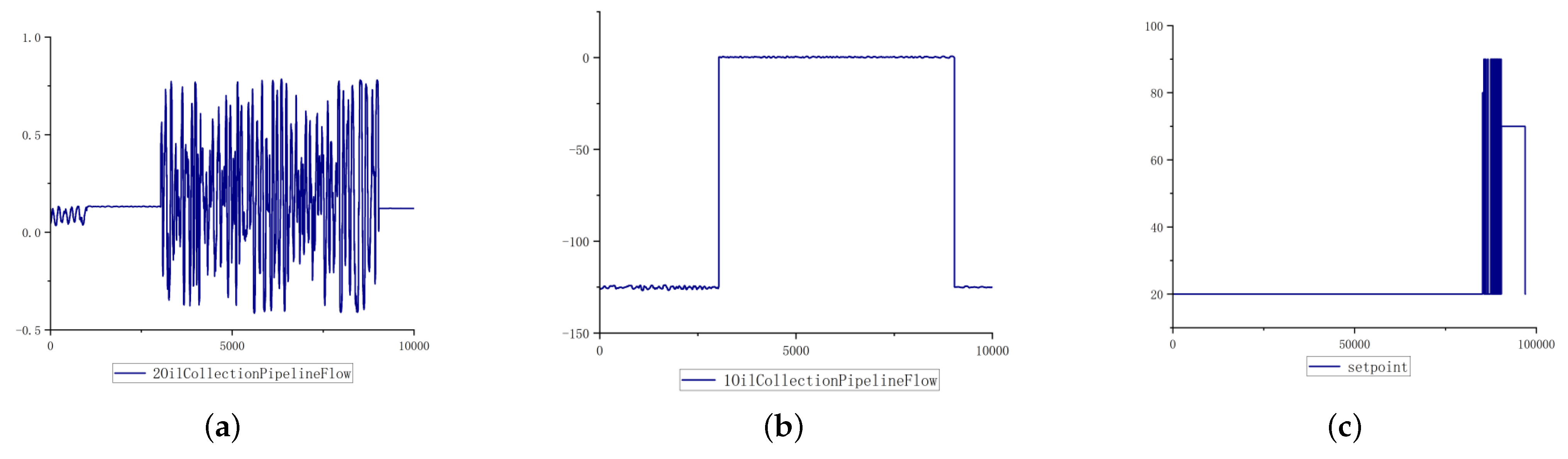
Take the oil dataset as an example. The attack sample dataset of an oil depot has certain temporal characteristics, so it is necessary to pay attention to the temporal relationship of newly generated samples in data generation. At the same time, the dataset includes the flow, pressure and other characteristics of each oil tank. The characteristics of industrial control attack samples will produce step jumps or oscillation fluctuations according to different types of attacks in different periods. Figure 1a is a feature of oscillation type change. The data fluctuates violently when attacked, which is a common fluctuation in industrial control attack sample data. Figure 1b is a feature of step type change. The data generate a huge step jump at the moment of attack. The data range changes significantly and remains unchanged within the duration of attack. Until the end of the attack, the data range returns to the normal range. The change trend of data before and after jump is similar. The specific trend is shown in the following formula:

The time sequence range of step type data are $t_0\sim t_{n-1}$, $t_n$, $t_{n+1}\sim t_m$, where $t_n$ is the time when the step jump occurs, $n+1<m$ and $m-(n+1)=(n-1)-0$:

$$S\left(y\right)=S(\frac{1}{n}\sqrt{\sum _{i=0}^{n-1}(y_{t_i}-y_{t_{n+i+1}})})$$

(1)

Data curve Q is bounded by $t_n$, and the changes of the two curves are similar. When $Q<S$ and $|{\overline{y}}_{t_0\sim t_{n-1}}-{\overline{y}}_{t_{n+1}\sim t_m}|>\epsilon$, the curve is said to have a step, where $\epsilon \gg {\overline{y}}_{t_0\sim t_{n-1}}$ or $\epsilon \gg {\overline{y}}_{t_{n+1}\sim t_m}$.

This classification of the underlying business data of industrial control is also applicable to the Singapore dataset. It comes from a real-life medium-sized water supply network, C-Town water system, established by iTrust, Network Security Research Center of Singapore University of Science and Technology. The system includes 1 independent reservoir, 5 valves, 5 pumping stations, 11 pumps, 7 storage tanks, 388 interfaces and 423 pipelines. The dataset has 130 feature dimensions, which can be divided into oscillation types and step type according to the fluctuation of time series data of each feature and whether there is step jump.

However, only the two classification methods for data expansion above are not applicable to the gas dataset. The Mississippi dataset comes from a set of SCADA systems based on all physical objects researched by Mississippi State University, in which the natural gas tank dataset is the underlying business dataset containing the attack. The natural gas data set has 26 dimensions, in which multiple feature data are in the form of pulses. Figure 1c shows the pulse type change feature, which is different from the step type change data value range. This feature constantly tampers with the data when being attacked, and the binary value jumps repeatedly to form the pulse change.

According to the characteristics of three kinds of industrial control underlying data, this paper studies the adaptive industrial control attack sample expansion algorithm based on GAN, to solve the sample generation problem of step type, oscillation type, and pulse type data.

3. Related Work

3.1. Time-Series Dataset Enhancement Algorithm

The industrial automation control abnormal dataset is a time-series dataset essentially. Although data types are diverse, the data enhancement methods they use have common design ideas, such as flipping, stretching, oversampling or adding noise. The enhancement effect of these methods is not satisfactory. Until the emergence of GAN in 2014, this situation was changed [9]. GAN was first used in the image field. Through the idea of a two person zero sum game, it can generate data that can not be distinguished by humans but can be judged by the model. The generated results are very similar to the original samples, and the generation efficiency is also improved. If this method is applied to the generation of abnormal data of an industrial control system, the generated negative samples are more similar to the positive samples. Thus, the authenticity of the generated samples is improved. After that, many improved methods of GAN began to appear.

In 2014, Mirza [11] proposed the CGAN model, but the quality of the generated data was not satisfactory. In 2015, LAPGAN [12] improved CGAN by introducing the concepts of Gaussian pyramid [13] and Laplace pyramid [14] in the field of image processing into GAN. This algorithm improves the convergence speed and the quality of the generated data, but it uses more computer memory. In the same year, Radford [15] used a convolution layer in GAN to make the generated pictures more similar and diverse. Its generator is 5-layer deconvolution, and its discriminator is 5-layer convolution. After that, the application of GAN gradually moves towards a broad field.

In 2016, Mogrend [16] proposed C-RNN-GAN, which is one of the first examples of using GAN to generate continuous sequence data. The generator of C-RNN-GAN is an RNN, and the discriminator is a bidirectional RNN, which allows the discriminator to obtain the sequence context in two directions. The f-GAN [17] proposed by Nowozins in 2016 solves the problem of the gradient of GAN easily disappearing when calculating the loss in training. This algorithm constructs the objective function of GAN according to the f-divergence of any convex function to enhance the stability of GAN. In 2017, LSGAN [18] appeared. It omitted the cross-entropy loss function and adopted the least square loss function, which improved the image quality, but the training was unstable. In 2017, Martin [19] proposed WGAN, which uses the Earth-Mover distance to calculate the similarity between the probability distribution of real data and the generated data. Although this method improves the stability of GAN. However, WGAN may fail in the process of algorithm convergence. Ref. [20] proposed WGAN-GP to solve the problems of gradient disappearance and parameter dispersing caused by weight clipping in WGAN, which uses a penalty mechanism instead of weight clipping to enforce Lipschitz constraint.

In 2018, Donahue [21] combined GAN with WaveNet to propose WaveGANs [21], which were used in unsupervised audio synthesis. In 2019, Zhu et al. [10] proposed the BiLSTM-CNN GAN on Nature for heart disease data detection. In the same year, Yoon [22] used the generative adversarial networks to generate time-series data; this algorithm considers both temporal features and static features and works well in multi-dimensional periodic time series data with large fluctuations, but it is not suitable for flat and disordered industrial underlying data.

In 2020, Ni [23] proposed Signature Wasserstein-1 (Sig-W1) to solve the problem of long time-series data increasing the dimension of generation modeling. This algorithm captures the time dependence of the time-series model and uses it as a discriminator in time-series GAN, establishing a conditional autoregressive feedforward neural network (AR-FNN) as a generator. However, the algorithm still can not solve the problem in which the step jump-points in the data attack samples of the industrial control underlying are ignored as noise.

The abnormal data set of industrial automation control has the characteristics of few jump points and similar data fluctuation trend before and after the jump points. In the iteration of data expansion based on GAN network, its characteristics will be ignored as data noise. To sum up, most of the existing GAN derived networks are more and more powerful in filtering data noise and better in gradient convergence. They will ignore the jump points of the three types of data of the industrial control underlying business data as noise points when the data iteration network updates parameters. However, the convergence speed of the basic GAN gradient is slow, the noise filtering ability is weak, and the characteristics of data jump can be preserved relatively well. In addition, most of the improved GANs for time-series data generation are only applicable to periodic data and have poor performance in disordered Industrial automation control data. In order to make the noise points not be ignored during data iteration, this paper uses the basic adversarial generation network as the main network of data generation.

3.2. Common Optimizer

Stochastic gradient descent (SGD) [24] is frequently updated with high variance, and its objective function will fluctuate violently. Although volatility allows SGD to jump to the new and potentially better local optima, it complicates the process of eventually converging to a specific minimum. The momentum method improves SGD by adding momentum in simulated physics. This algorithm improves the convergence speed while preserving the volatility of the SDG method. Therefore, the momentum optimizer is more suitable for the characteristics of fluctuations in a certain range of oil depot data, but it is not suitable for data with significant jump at a certain time. Both SGD and momentum perform gradient descent and parameter updating at a certain step in the direction of gradient convergence. In addition, in the process of iteration, they gradually reduce the influence of noise, and finally make the gradient converge. However, the step jump point in the oil depot data will be mistaken as noise data, resulting in the generation result showing a gradual rise or fall curve change, and the step change of the generated data is far from that of the original data. Therefore, the better the gradient descent effect, the harder it is to retain the step effect of the data.

The main principle of the Adagrad algorithm is to adapt the learning rate to the parameters. This algorithm uses a large learning rate to deal with features that occur less frequently and uses a small learning rate to deal with features that occur more frequently. The Adagrad algorithm greatly improves robustness based on SGD and is very suitable for processing sparse data. The RMSprop algorithm adds an exponential moving weighted average to improve the Adagrad algorithm, which solves the problem of too small learning rate in the later stage. Adam optimizer [25] combines the advantages of Momentum and RMSprop, and it adds deviation correction, so that the Adam optimizer can greatly reduce the volatility and obtain better results in the early stage of training. However, it can only make the model learn the jump-point in the early stage, and will still ignore the jump-point as noise in the later stage.

Therefore, aiming at the above problems, this paper improves the Adam optimizer. This method amplifies the influence of jump data on gradient updating, and then realizes step jump of data when generating data.

4. Method

4.1. Notation Explanation

In the adaptive industrial control attack sample expansion algorithm based on GAN, certain notations were defined and their meaning was explained, as it is shown in

Table 1. Notations and their meanings.

Notations	Meanings
$d_{max}$	the maximum value of all the data of the current feature
$d_{min}$	the minimum value of all the data of the current feature
$x_t$	the data of this moment in the current data fragment
$x_{t-1}$	the data of previous moment in the current data fragment
$y_1$	the judgment result of the turning point
$d_{avg}$	the average of all data of the current feature
D	matrix with the same size as $d_{avg}$
$X_t$	the current data fragment
$X_{t-1}$	the current data fragment
$y_2$	the turning point judgment result
t	the number of updates
${\theta }_t$	the update step of Adam t
${\theta }_{t-1}$	the step of the previous iteration
$\alpha$	the learning rate
${\widehat{m}}_t$	the momentum
$\sqrt{{\widehat{v}}_t}$	the exponential moving average of the gradient
∈	a constant
$K\left(e^{(-\Delta x)}\right)$	a decreasing function of the change of sample eigenvalues
$y_3$	is the judgment result of pulse position
$\Delta t$	the length of the pulse

.

4.2. Data Generation for Oscillation Type

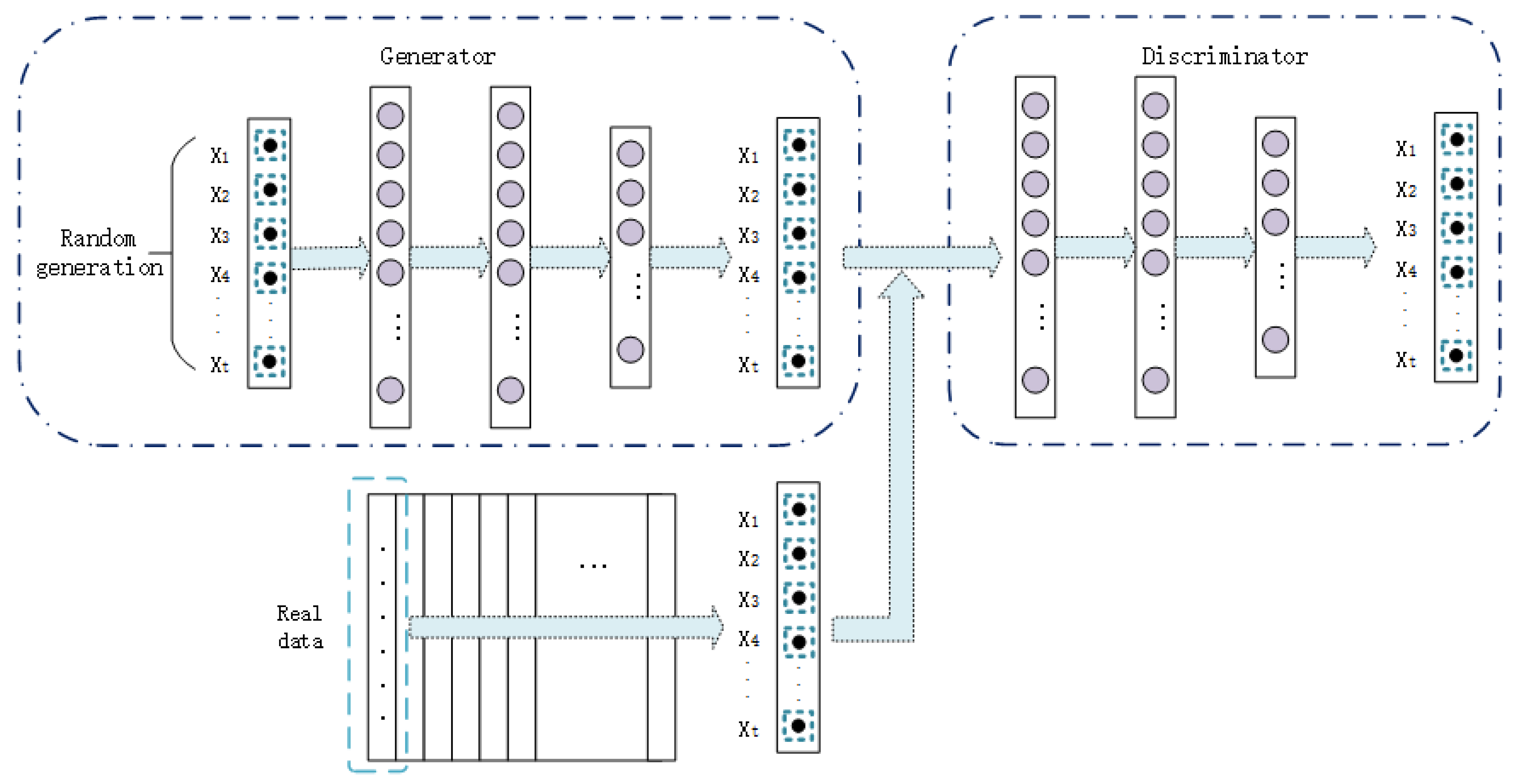
The main network structure of data generation is the original generative adversarial network. As shown in Figure 2, the discriminator consists of three fully connected layers, and leakyRelu is used as the activation function after calculation for each layer of the first two layers. The activation function of the last fully connected layer is sigmoid. The generator is also composed of three full connection layers, and relu is used as the activation function after calculation of each of the first two layers. The activation function of the last full connection layer is tanh.

As shown in Figure 1a, for oscillation types data, this paper selects the momentum optimization method as the optimizer. Compared with Adam that is widely used in various projects, momentum has a strong ability in preserving the fluctuation of oscillation type data. In addition, its convergence speed is higher than SGD.

4.3. Data Generation for Step Type

As shown in Figure 1b, the step type data will change at a certain time, and the changed waveform is very similar to the waveform before the step change. This situation will be considered as noise in the traditional generative countermeasure network. In the process of network iteration, the variable step size of iteration is modified by momentum and average gradient, so that the generated attack samples are smoother and the influence of step is removed as far as possible. In order to generate step type data, this paper is divided into two steps to improve the generative adversarial network: (1) Searching for Jump Points and (2) Improved Adam optimization methodology.

4.3.1. Searching for Jump Points

The step jump points of different feature data have different positions. This paper uses Formula (2) to calculate the jump points:

$$y_1=\left\{\begin{array}{c}1,(d_{max}-d_{min})/2<\left|x_{t-1}-x_t\right|\\ 0,(d_{max}-d_{min})/2\ge \left|x_{t-1}-x_t\right|\end{array}\right.$$

(2)

If the turning point judgment result is 1, the current data segment contains step jump points.

Jump points may occur between fragments except in the middle of fragments, so Formula (3) is used to calculate between fragments:

$$y_2=\left\{\begin{array}{c}1,D/2<\left|X_{t-1}-X_t\right|\\ 0,D/2\ge \left|X_{t-1}-X_t\right|\end{array}\right.$$

(3)

$$d_{avg}=(d_{max}-d_{min})/2$$

(4)

If the turning point judgment result is 1, a step jump occurs between the previous data segment and the current data segment.

4.3.2. Optimization Algorithm for Adam

The core formula of Adam optimization method is Formula (5) [25]:

$${\theta }_t={\theta }_{t-1}-\alpha \ast {\widehat{m}}_t/(\sqrt{{\widehat{v}}_t}+\in )$$

(5)

In order to realize the jump of the generated reserved value of attack samples, the adjustment factor is added in Formula (5), so that it is instantaneously decoupled from the moving average of momentum and gradient index when it encounters step jump, and becomes Formula (6):

$${\theta }_t={\theta }_{t-1}-\alpha \ast K(e^{(-\Delta x)})\ast {\widehat{m}}_t/(\sqrt{{\widehat{v}}_t}+\in )$$

(6)

The larger the change of eigenvalue, the smaller the value of function $K\left(e^{(-\Delta x)}\right)$. The main steps in the optimizer are shown in

Table 2. The main steps in the optimizer.

Number	Events
1	Initialize learning rate, attenuation rate, update times, cumulative gradient and cumulative gradient square.
2	Receive current network parameters. If it is the first update, save the network parameters of each layer of the model.
3	Update training times and calculate gradient.
4	Calculate the exponential moving average of gradient value and the exponential moving average of square gradient value.
5	Correct deviation.
6	Update parameters with Equation (6).
7	Repeat the above steps 2 to 6 until the training is completed. If the judgment result of the turning point is 1, the network parameters of each layer of the current model are saved after Step 2, and replaced by the previous record.

.

4.4. Data Generation for Pulse Type

As shown in Figure 1c, due to the short pulse length of the pulse type data itself and the large jump degree between the data, it cannot be classified as the above oscillation and step types. This paper adopts the step-by-step generation method. Firstly, the positive sample generated by the generative adversarial network is used as the basic trend of the negative sample, and then the location of the pulse is calculated through Formula (7) for the original data, and the pulse length is calculated:

$$y_3=\left\{\begin{array}{c}1,\left|x_{t-1}-x_t\right|\ne 0\\ 0,\left|x_{t-1}-x_t\right|=0\end{array}\right.$$

(7)

When $y_3$ is 1 for the first time, it is the start position of the pulse; when the second time $y_3$ is 1, it is the end position of the pulse. Between two times $y_3$ is 1, the pulse length can be obtained.

The value of pulse position t and pulse length $\Delta t$ is converted to percentage. Then, read the pulse position value and generate new pulses. The sample distribution is calculated by the probability formula, and the positions of the high and low binary values in the pulse are arranged according to the sample distribution to generate a new pulse. Finally, according to the location and length of the original data, the pulse is inserted into the basic trend to form a new attack sample. 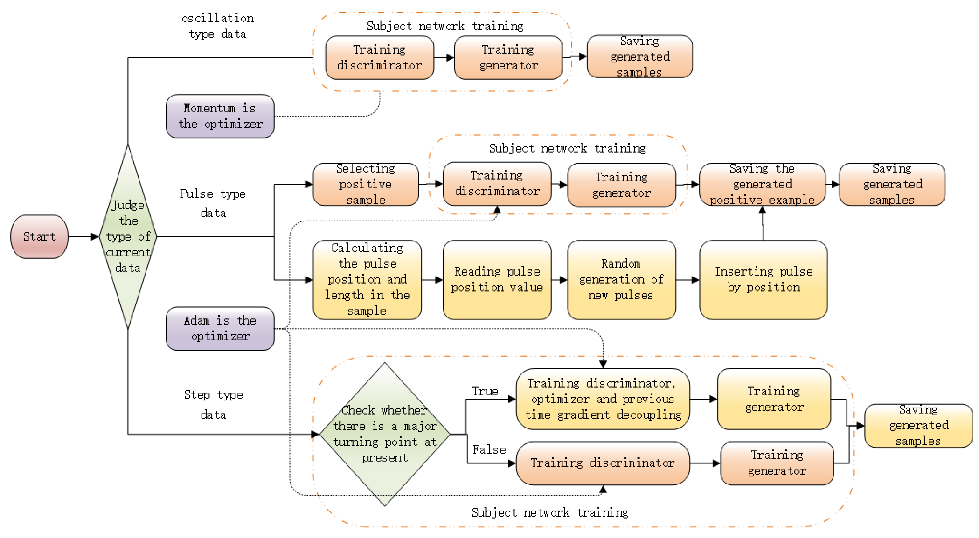Figure 3 shows the overall flow chart of the algorithm.

5. Experimental Validation

The experimental environment is a Windows 10 system, the CPU is 11th Gen Intel(R) Core(TM) i7-11800H @ 2.30 GHz 2.30 GHz, the GPU is NVIDIA GeForce RTX 3050 Laptop GPU and the memory of GPU is 8 GB.

The purpose of the experiment is to find an algorithm suitable for the sample data of the industrial automation control underlying attack and the only evaluation index of the algorithm is the similarity between the generated sample and the original data.

There are 172,804 pieces of data and 130 characteristic values in the Singapore dataset, including 162,827 positive samples and 9977 attacked data. Data collection lasted for three days and was attacked by 12 types of attacks.

There are 158,175 pieces of data and 26 characteristic values in the gas dataset, including 61,156 positive samples and 97,019 attacked data. It is subject to seven types of attacks, including command injection, response injection, denial of service (DoS) and reconnaissance.

There are 131 characteristic values in the oil dataset, including oil pump inlet pressure, oil pump outlet pressure, tank liquid level, tank pressure, tank temperature, filter differential pressure, etc. There are seven types of attacks on data. This experiment mainly uses 10,030 attack samples as seed attack samples to expand data.

The control group of our experiment is GAN, DCGAN, BiLSTM-CNN GAN and TimeGAN. Manhattan coefficient is used to evaluate the similarity of the generated dataset.

5.1. Optimizer Selection Experiment

The experimental parameter batchsize is set to 50 and epoch is set to 20. This paper randomly generates a noise incoming generator with a length of 1000. The generator is composed of three full connection layers, and the number of neurons in each layer is 256. Between layers, ReLU is used as its activation function. Finally, the generated data are distributed between [−1,1] through Tanh activation. The number of layers and neurons of the discriminator are consistent with that of the generator. LeakyReLU is used as an activation function in the middle. In addition, the data activated through Sigmoid will be mapped to the region of [−1,1].

According to the change trend of three characteristics, our experiment uses five common methods, including Adam, Adagrad, momentum, SGD and RMSprop.

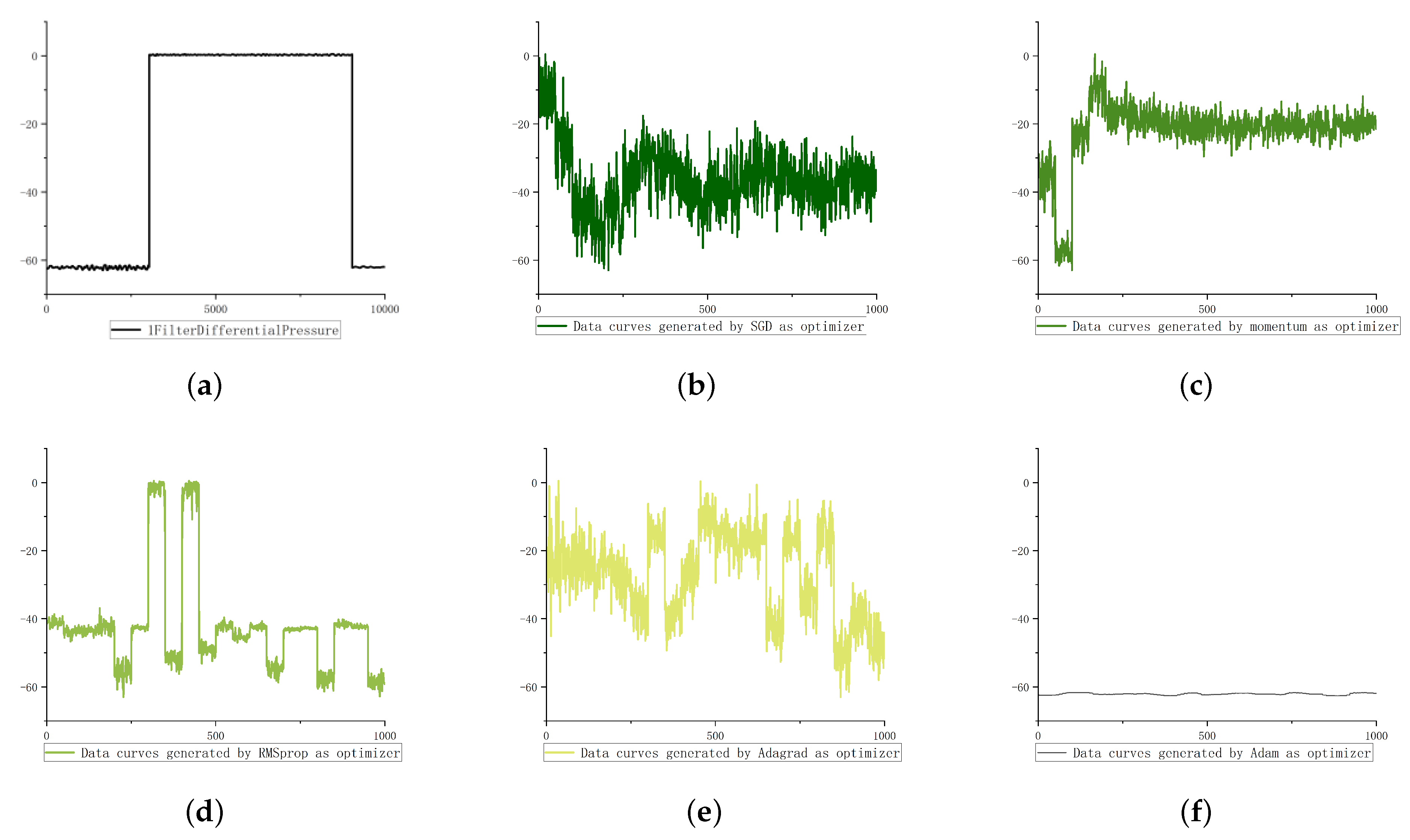
5.1.1. Oscillation Type Data Generation

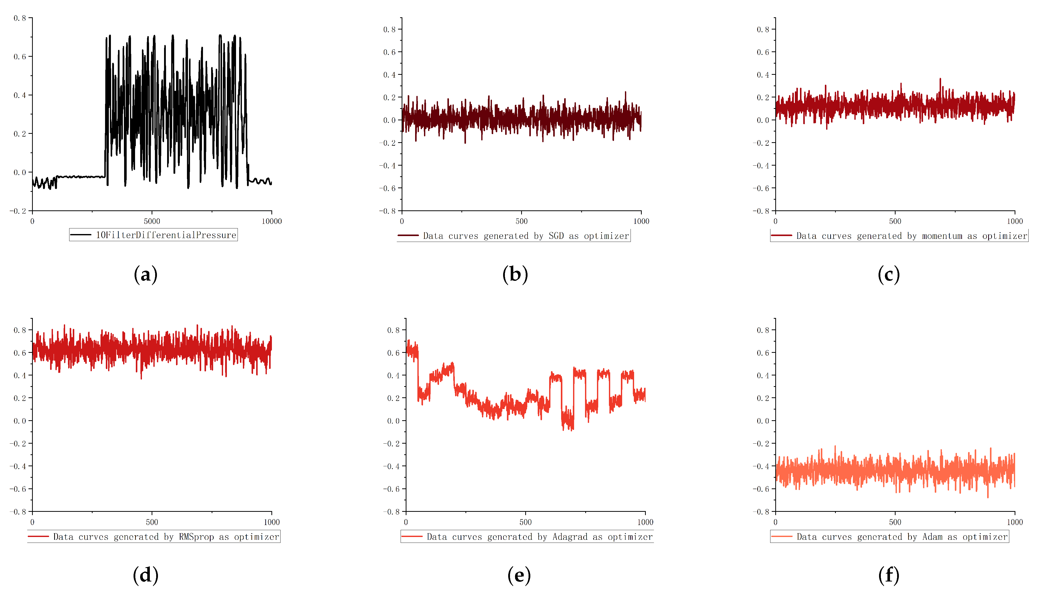
As shown in Figure 4, Figure 5 and Figure 6, the step type data and oscillation type data come from the 1-filter-differential-pressure feature and 10 filter differential pressure feature of the oil dataset. Pulse data come from the gas dataset.

As shown in Figure 4, the fluctuation trend of the data generated by using adagrad and Adam optimization methods is far from the original data; the data generated by the rmsprop optimization method is far from the original data in value range; however, the data generated by SGD and momentum optimization methods are more similar to the original data than the other three. Therefore, aiming at the change of oscillation characteristics, this paper chooses momentum as its optimizer.

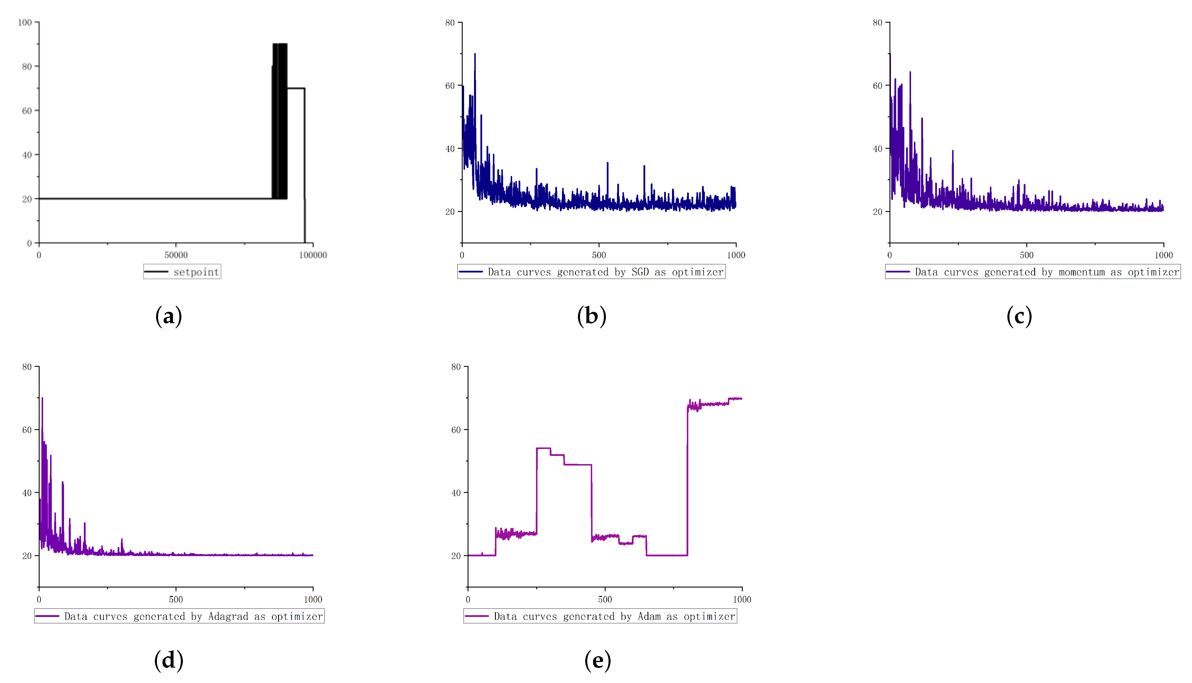
5.1.2. Step Type Data Generation

As shown in Figure 5, except for the step jump in the value range, the overall fluctuation trend of the step type data in the original data is very smooth. Only the data generated by Adam optimization method have the most similar fluctuation trend, and the results of other optimization methods are far from it. Therefore, aiming at the change of step characteristics, this paper improves the Adam optimization method and applies it to the generative countermeasure network.

5.1.3. Pulse Type Data Generation

RMSprop failed to generate data due to the disappearance of gradient during training, so this paper does not put it into the comparison results. As shown in Figure 6, compared with the data generated by other optimization methods, the fluctuation trend of the data generated by Adam optimization method is most similar to that of the original pulse type data. In view of the change of pulse characteristics, this paper chooses the Adam optimization method as its positive example sample generator. It takes the generation result of positive samples as the basic trend of negative samples, and then carries out pulse embedding.

5.2. Experimental Results of Related Algorithms

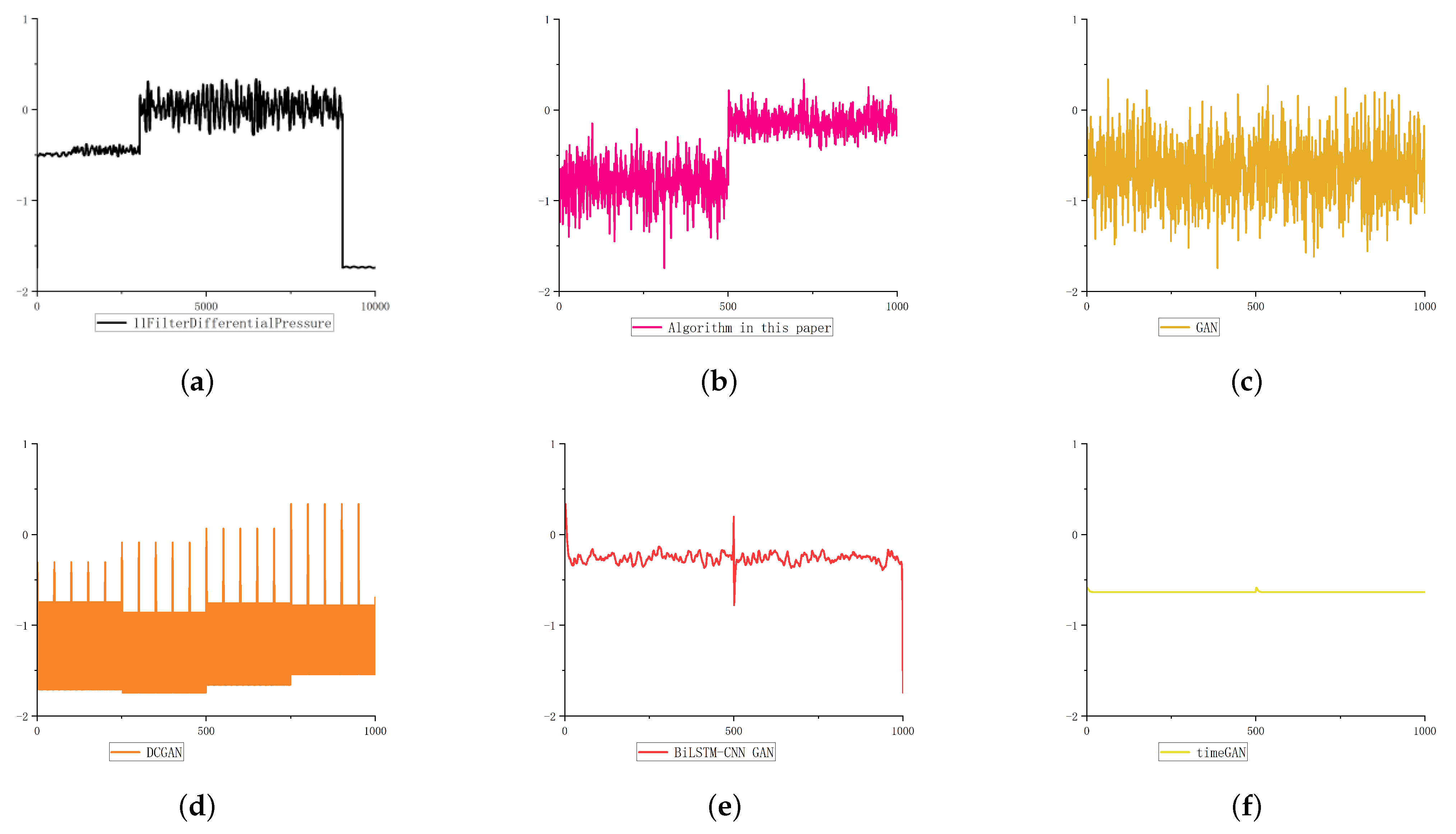
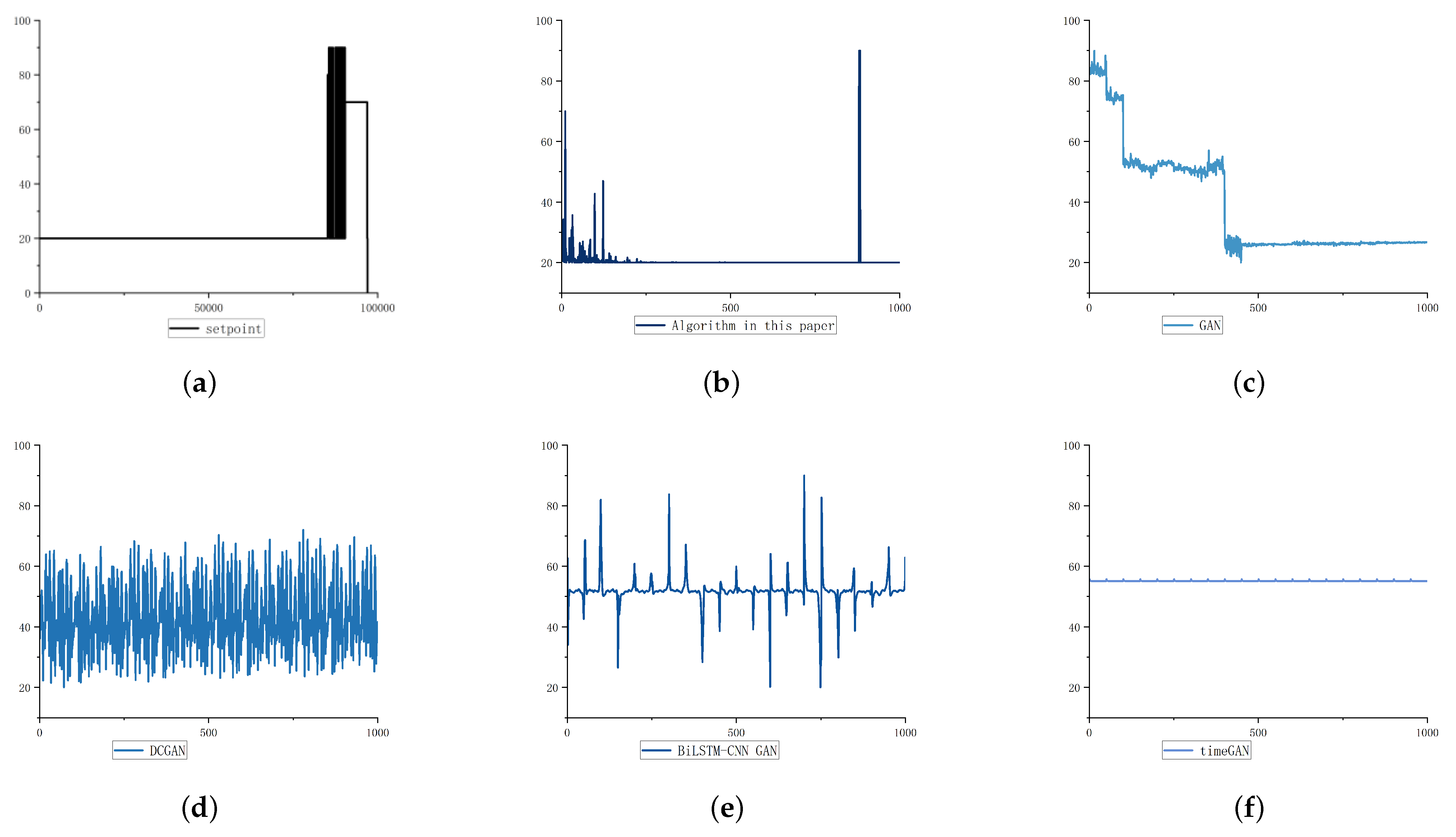
This paper conducts comparative experiments with four different GANs on three different datasets. Except for the fact that batchsize is 500 and epoch is 2, other parameters of the experiment are the same as those of the optimizer selection experiment. The experimental comparison algorithms include GAN, BiLSTM-CNN GAN, DCGAN and TimeGAN. The jump point in the characteristic change trend often means that the attack occurs. Therefore, the overall trend of feature data and the position of jump point are the key to data generation in this paper.

5.2.1. Oscillation Type Data Generation

For oscillation type data, the four comparison algorithms use SGD as the optimizer. As shown in Figure 7, compared with DCGAN, Bilstm-CNN GAN and TimeGAN, which have better effects in image generation and time-series data generation, the algorithm in this paper is more similar to the original data in terms of the change trend and jump position of the generated data in terms of the oscillation type characteristics of the negative sample of the industrial control underlying business data.

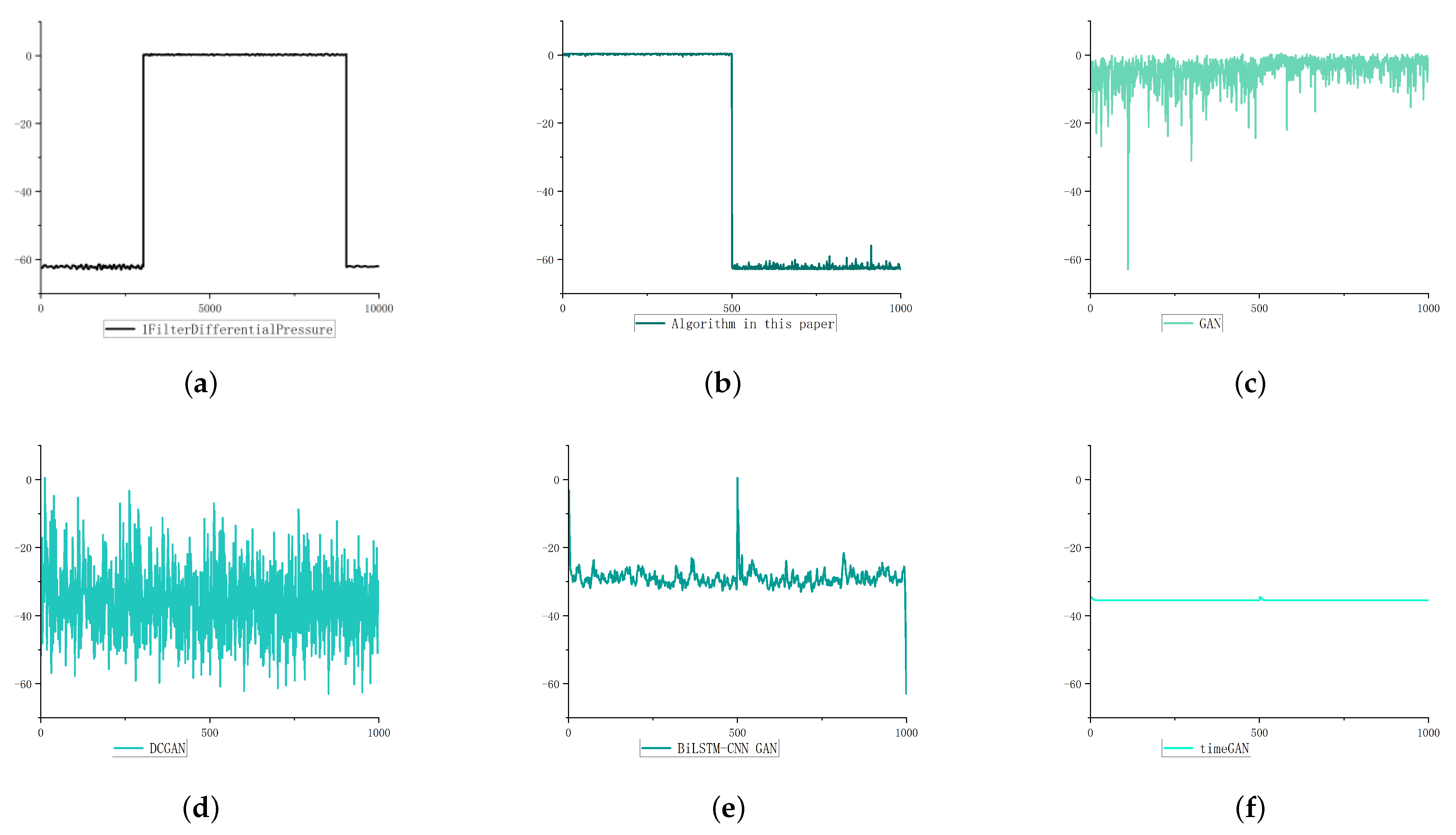
5.2.2. Step Type Data Generation

For step type data, the Adam optimization method is used as the optimizer to compare GAN and DCGAN in the algorithm; Bilstm-CNN GAN and TimeGAN use the improved Adam optimization method as the optimizer. As shown in Figure 8, compared with dcgan, bilstm CNN Gan and TimeGAN, which have better effects in image generation and time series data generation, the algorithm in this paper can learn the step change of the original data in terms of the step feature change of the negative sample of the industrial control underlying business data. Our results are more similar to the original data in terms of the change trend and jump position of the generated data.

5.2.3. Pulse Type Data Generation

For pulse type data, the four comparison algorithms use SGD as the optimizer. As shown in Figure 9, compared with DCGAN, Bilstm-CNN GAN and TimeGAN, which have better effects in image generation and time-series data generation, the algorithm in this paper is more similar to the original data in terms of the change trend and jump position of the generated data in terms of the ladder type characteristics of the negative sample of the industrial control underlying business data.

In addition, as shown in

Table 3. Comparison of similarity between generated data and seed data (Manhattan distance).

Names	Mississippi Gas Dataset	Singapore Water Plant Dataset	Real Oil Depot Dataset
GAN	42,160.32	23,403.22	9228.57
DCGAN	329,862.87	23,509.43	5351.57
BiLSTM-CNN	29,691.46	17,290.25	5693.17
TimeGAN	72,557.52	57,903.48	5550.95
Ours	24,019.34	14,213.40	4886.39

, this paper expands all the features of the three datasets and compares the similarity of the five algorithms on each dataset by calculating Manhattan distance.

As shown in Table 3, the evaluation standard of the algorithm is the average value of each characteristic Manhattan value in the dataset. Smaller Manhattan values indicate more similarity to the original dataset. In the expansion of sample data of industrial control underlying business data attack, the effect of this algorithm is better than the other four comparison algorithms.

6. Conclusions

In order to solve the problem in which the attack sample data of the underlying business data are scarce in the industrial automation control system, this paper proposes an adaptive generation algorithm of industrial control sample based on GAN. The experimental results show that our algorithm is more targeted for the generation of different characteristic time-series data, and it has a higher degree of similarity with the original data.

The attack sample data of the underlying business data are related in the industrial automation control system. In the process of data generation, how to learn the relationship between features more accurately is still a problem to be solved.