Tight Maneuvering for Path Planning of Hyper-Redundant Manipulators in Three-Dimensional Environments

Abstract

An effective path-planning algorithm in three-dimensional (3D) environments based on a geometric approach for redundant/hyper-redundant manipulators are presented in this paper. The method works within confined spaces cluttered with obstacles in real-time. Using potential fields in 3D, a middle path is generated for point robots. Beams are generated tangent to the path points, which constructs a basis for preparing a collision-free path for the manipulator. Then, employing a simply control strategy without interaction between the links, the motion planning is achieved by advancing the end-effector of the manipulator through narrow terrains while keeping each link’s joints on this path until the end-effector reaches the goal. The method is simple, robust and significantly increases maneuvering ability of the manipulator in 3D environments compared to existing methods as illustrated with examples.

1. Introduction

Redundant manipulators are known as having an infinite number of solutions to the joint variables [1]. Although there are serious problems implementing and controlling a redundant manipulator [2], they have great mobility resulting in collision-free path planning among obstacles [3] as performing scrutiny, maintenance or rectifying tasks [4]. Redundant manipulators achieve such challenging tasks by means of extra degrees of freedom (DOF) [5,6,7].

There are some useful definitions. If a goal point is given as a task to reach for the end-effector, the path-planning problem is reduced to finding a feasible joint path array. On the other hand, if the tool-tip path is already obtained beforehand, a feasible joint path array is found by means of redundancy resolution [5]. Motion planning is considered in two groups: high-level and low-level planning. Low-level planning is about collision-free planning while high-level planning is about collision avoidance [8].

While potential fields, cell decomposition and roadmaps are well-known and well-established motion planning methods, motion planning is addressed in different ways by some path-planning methods [9,10,11]. These include methods utilizing kinematic or geometric representation of the manipulator [12] in which redundancy resolution is combined with path-planning through finding a solution to a differential equation connecting task space motion and the joint [5]. Although a systematic categorization of motion-planning methods is somewhat difficult due to wide variety in the literature [13], the motion-planning methods could be considered in four groups: Geometric, curve based, Jacobian based and path tracking [14].

A backbone curve is designed with the ability of mapping the continuous highly redundant manipulator onto this curve. But the performance suffers with high number of redundant links. Also, the method is unable to handle backbone curves with large curvature [15]. In [16], a method by means of numerical potential fields is developed navigating the manipulator among obstacles in the absence of collision. The method puts certain points on manipulator links, which creates virtual torque at the joints to steer the manipulator. But it becomes slower when the number of control points on a link increases. The potential field defined in the workspace is coupled with Lagrange’s equations of motion providing paths avoiding obstacles for path-planning of a snake robot [17]. There are also potential field based methods such as improved artificial potential field method [18], generalized potential field method [19] and harmonic potential field method [20] to plan the safe trajectory and avoid obstacle for hyper-redundant manipulators in 3D environments. There also exist time-optimal trajectory planning methods for hyper-redundant manipulators in 3D workspaces by reducing the problem to an optimization problem [21,22]. The problem is solved via Genetic Algorithm (GA) in the proposed methods. However, Hyper-Bump Surface concept is used for trajectory planning in [21] while the kinematical constraints of the manipulator and the obstacles are considered in [22]. It becomes more difficult to map a manipulator with relatively long link lengths onto its curve, which results in colliding with the obstacles [23]. There are path-planning methods using optimal techniques [24,25], sensory data [26], bump-surfaces notion [27] and backtrack-free planning [28]. Another path-planning algorithm is proposed for a multi-arm space robot which is capable of maneuvering on the exterior of a large space station. The kinematics of the hyper-redundant manipulators are formulated and the joint trajectories are calculated via a pseudoinverse solution [29].

A snake manipulator with links made of a Stewart platform is mapped onto serpenoid curves. The platform with pneumatic cylinders is inherently heavy and only allows each link to move by a small amount that results in poor curve matching [30]. A sort of mapping utilizing sub-paths with the perimeter of a half ellipse is developed in [31] while swarm optimization with proper waypoints exploits a fitness function for inverse kinematics [32].

A highly redundant manipulator whose links are driven by electromagnetic energy in a bi-stable way is suggested [33]. A common way of steering hyper-redundant manipulators with discrete modules is to actuate it by cables [34,35,36]. There also exists a collision-free path-planning algorithm called Swinging Search and Crawling Control to explore the complex pipeline environments for snake-like redundant manipulators [37]. A modified modal method which defines the spatial backbone of the manipulator via a mode function is proposed to solve the mission-oriented inverse kinematics considering the mission requirement and workspace [38].

In order to resolve the problem of angle constraint for hyper-redundant manipulators, a Rapidly-Exploring Random Tree (RRT) based path planning algorithm is proposed and applied to a cable-driven hyper-redundant manipulator with 17 degrees of freedom [39]. The actuation system and the control of hyper-redundant robots are simplified for under-actuated snake robots [40]. Another approach is presented for the collision avoidance of hyper-redundant manipulators in narrow spaces and applied to a hyper-redundant manipulator consisted of four pairs of double Universal-Cylindrical-Revolute parallel mechanisms [41].

A new approach is described in [42] based on a global path finding algorithm for the manipulator using Laplacian potential fields along with a simple local geometrically based algorithm featuring repelling obstacles, which maximizes the use of maneuvering space.

There are so many different ways of mapping manipulator links onto the path or path following for planning purposes as documented above. However, mapping the manipulator onto the path has a major drawback: if the link lengths compared with curvatures of the curves of the path are longer, the robot is jammed amid obstacles even if huge free space resides to maneuver. A solution is offered to this problem in [43] by joining the beams in [44] and the middle points in [45], which leads to extraordinarily maneuvering competence for redundant/hyper-redundant manipulators. In this paper, we come up with a real-time algorithm that is capable of achieving path planning and obstacle avoidance including 3D environments.

The paper is organized as follows; Section 2 explains the generation of the middle path as the benchmark environment is described in Section 3. The proposed algorithm is presented in Section 4 in all aspects. In Section 5, exemplary computer simulations are provided in 3D environments with illustrations. Discussions on the proposed algorithm and future work are given in Section 6. Finally, conclusions are reported in Section 7.

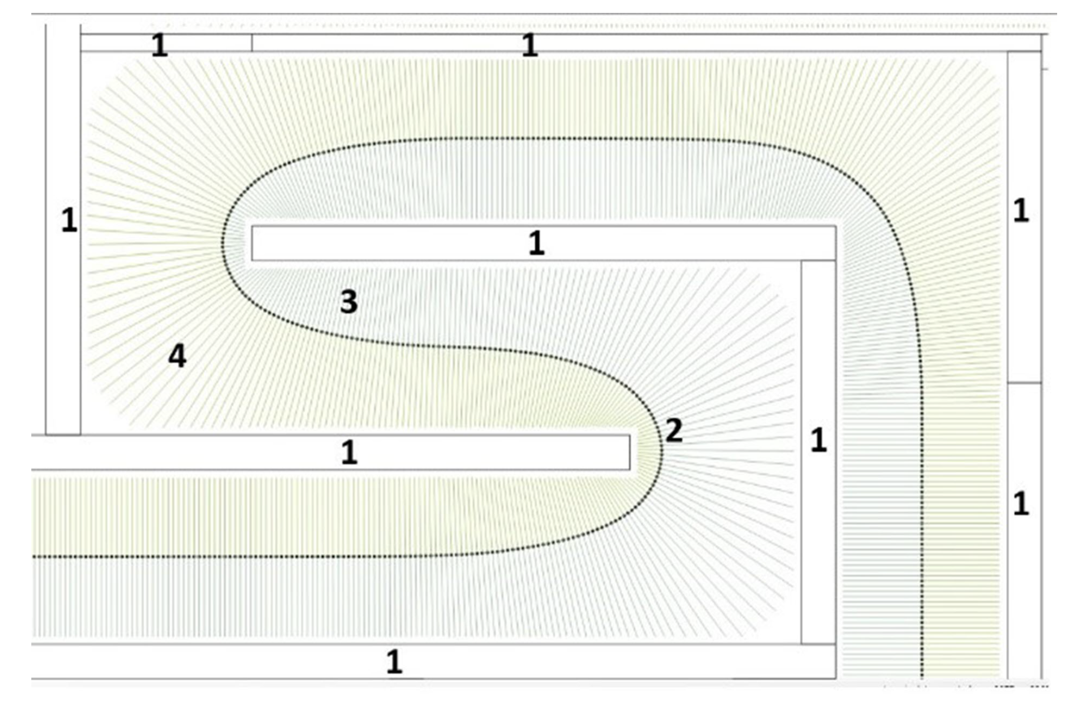
2. Potential Fields: Generating the Global Middle Path

The algorithm presented here is developed by using the information gathered from the global middle path from the robot tip to the goal point through obstacles. In other words, it is not the path that the links of the manipulator follow in the proposed algorithm. It only needs middle path points to place beam lines. The middle path may be generated by means of any global path-planning methods. Despite the alternative methods in the literature, numerical potential fields are a well-developed method without local minima. That is why, the Laplace equation is used to have information on the workspace for navigation purposes in developing the algorithm. Motion planning is carried out on top of that. For this reason, the potential field method is used and briefly explained in this section.

A scalar potential driven by Laplace’s equation under Dirichlet boundary conditions is expressed by

$${\nabla }^{2}u=0$$

(1)

Equation (1) is on a domain $\mathsf{\Omega }$ where the boundary of $\mathsf{\Omega }$ consists of the boundaries of all obstacles and the goal point. The goal point is given a very small number while the obstacle points including boundary points excluded in the calculation. The workspace $\mathsf{\Omega }$ is represented by a grid of certain dimensions. The partial equation represents the Laplace equation on equally spaced and connected grid as below.

$$u_{(i,j)}=\frac{u_{(i+1,j)}+u_{(i-1,j)}+u_{(i,j+1)}+u_{(i,j-1)}}{4}$$

(2)

where i and j are grid positions in the x and y directions, respectively. An iteration procedure using Equation (2) is performed on the grid to calculate field values at all points. A handful number of iterations are done to obtain field values at grid points. Following these values results in reaching the goal. Nevertheless, the path obtained is coarse due to path points placed on a discrete grid and is not very useful. For this reason, values within the square grid need to be accessed via the linear interpolation. Then, the direction of the largest descent $\alpha$ is calculated using Equation (3) as shown in Figure 1. Therefore it can be reached from the point of $p_k$ to the point of $p_{k+1}$ via vector $L_k$ in a two-dimensional (2D) environment. So, a collision-free path which is comprised of points for a point robot is obtained [44].

$$\alpha =arctan2\left(\frac{u_{(i,j-1)}-u_{(i,j+1)}}{u_{(i-1,j)}-u_{(i+1,j)}}\right)$$

(3)

Having obtained the path points, a much smoother path is attained by means of a numerical calculation method called windowing.

Calculating potential field in 3D environment is similar to calculating in 2D environment. L is the length of the cube representing the length of the side of the environment and N is the number of sections of this length. Grid values of the potential field are given below.

$$\begin{array}{cc}\hfill dx=dy=dz& =h=L/N\hfill \\ \hfill & u_{i,j,k}=u(x_i,x_j,x_k):i,j,k\in [0,N]\hfill \\ \hfill u_{i,j,k}=& \frac{u_{i-1,j,k}+u_{i+1,j,k}+u_{i,j-1,k}+u_{i,j+1,k}+u_{i,j,k-1}+u_{i,j,k+1}}{6}\hfill \\ \hfill & \frac{{\partial }^2}{\partial x^2}u(x_i,y_j,z_k)\approx \frac{u_{i-1,j,k}-2u_{i,j,k}+u_{i+1,j,k}}{h^2}\hfill \end{array}$$

(4)

Using Gauss-Seidel method, Equation (5) is obtained as follows;

$$u_{i,j,k}^{m+1}=\frac{1}{6}(u_{i-1,j,k}^m+u_{i+1,j,k}^m+u_{i,j-1,k}^m+u_{i,j+1,k}^m+u_{i,j,k-1}^m+u_{i,j,k+1}^m)$$

(5)

where i, j and k are grid positions in the x, y and z directions, respectively and m is the iteration number.

Calculation of the direction of the largest descent is also similar for 3D environments. In addition to $\alpha$ value, $\beta$ value is required from newly obtained line of $p_{k}d$ and the line of $p_{k+1}d$ which is the difference of the potential field in the direction of z as shown in Figure 2. Therefore it can be reached from the point of $p_k$ to the point of $p_{k+1}$ via vector L in a 3D environment.

The potential value at any point between the grid points can be easily calculated with the 3D linear interpolation formula given in Equation (6). Thus, smoother paths are obtained by using the values (V) on the cube as shown in Figure 3.

$$\begin{array}{c}\hfill V_{xyz}=V_{000}(1-x)(1-y)(1-z)+V_{100}x(1-y)(1-z)+V_{010}(1-x)y(1-z)+V_{001}(1-x)(1-y)z+\\ \hfill V_{101}x(1-y)z+V_{011}(1-x)yz+V_{110}xy(1-z)+V_{111}xyz\end{array}$$

(6)

3. Benchmark Environment

The maneuvering capability expressed mathematically via a benchmark workspace in [44] is shown in Figure 4. Index l in Equation (7) gives a measure about the maneuvering ability where $l_{max}$ represents geometrically possible maximum link length while $l_{link}$ represents the link length. The maximum value of l is 1.0.

$$l=\frac{l_{link}}{l_{max}}$$

(7)

4. The Algorithm

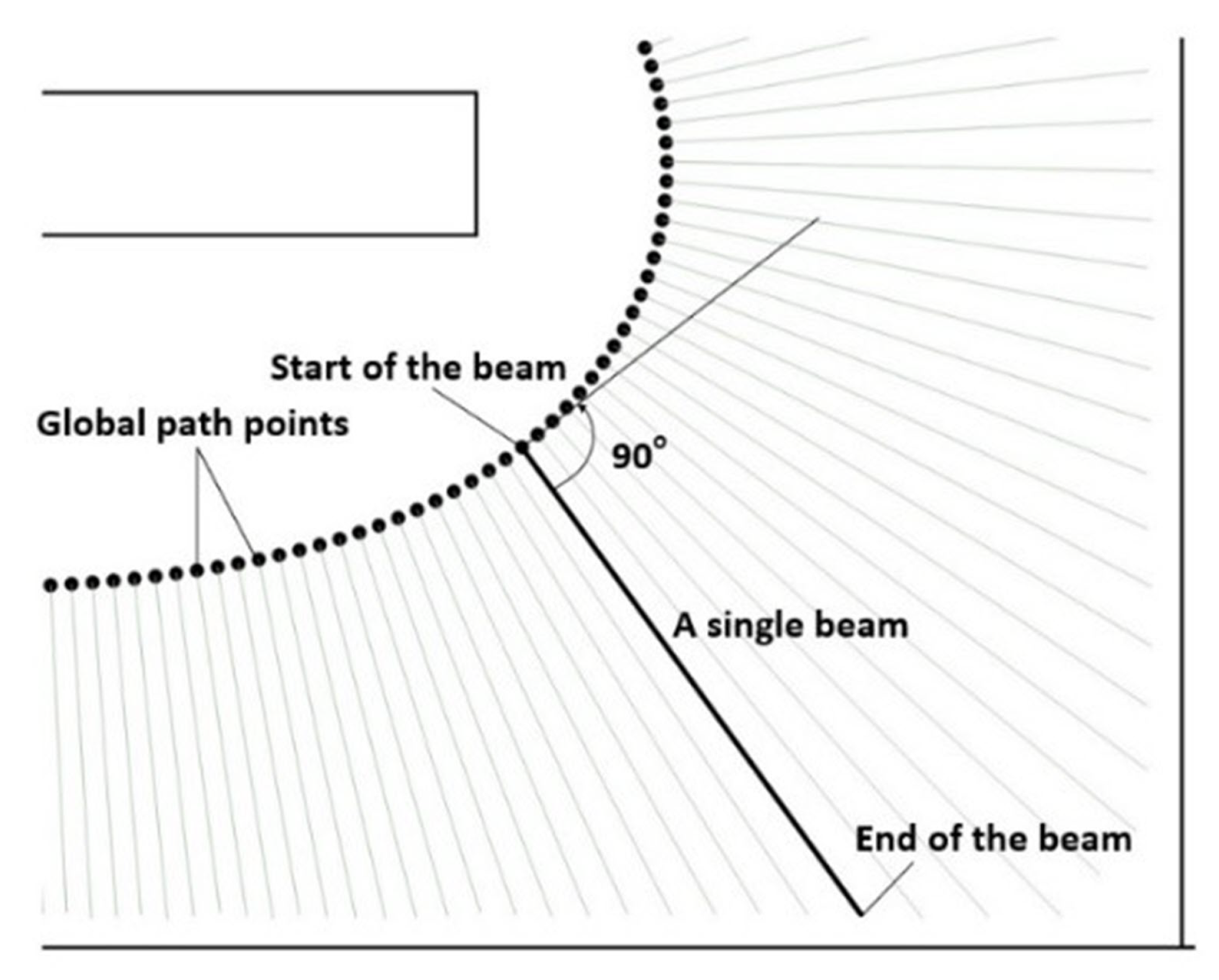
4.1. Obtaining the Global Middle Path and the Beams

Using the potential field, a global path consisting of points in the middle of the free space from the start point to the goal point through obstacles is generated. It is essential to smooth this path, which is done by means of windowing. Figure 5 shows a portion of this smooth path numbered as 2 and positioned in the middle of the free space. In this figure, the obstacles are numbered as 1 and the right beams are numbered as 3 and the left beams are numbered as 4. This path contains all the data required for the path planning of the manipulator.

Having the path, the beams are generated. Each beam starts from its path point and ends at the obstacle border. The angle between the beam and the path is 90${}^{\circ }$. In Figure 6, a right beam is shown. The same procedure is applied to the left beams. If the beam reaches its maximum length before reaching an obstacle border, it ends at that length. Especially critical regions generate short beam lengths. As seen in Figure 5, the area the beams cover is free space where the manipulator must be confined. However, since the tight maneuvering is required, only some portions of this free space must be used.

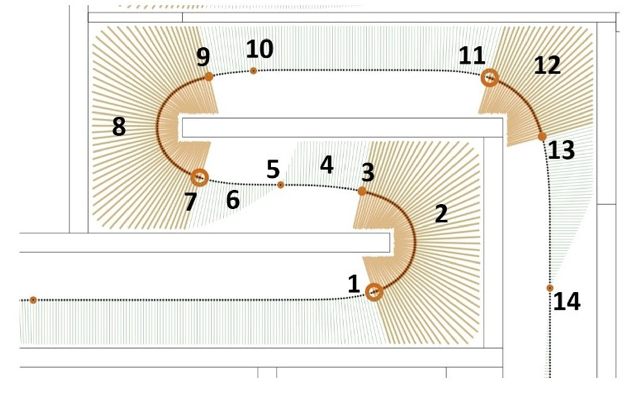
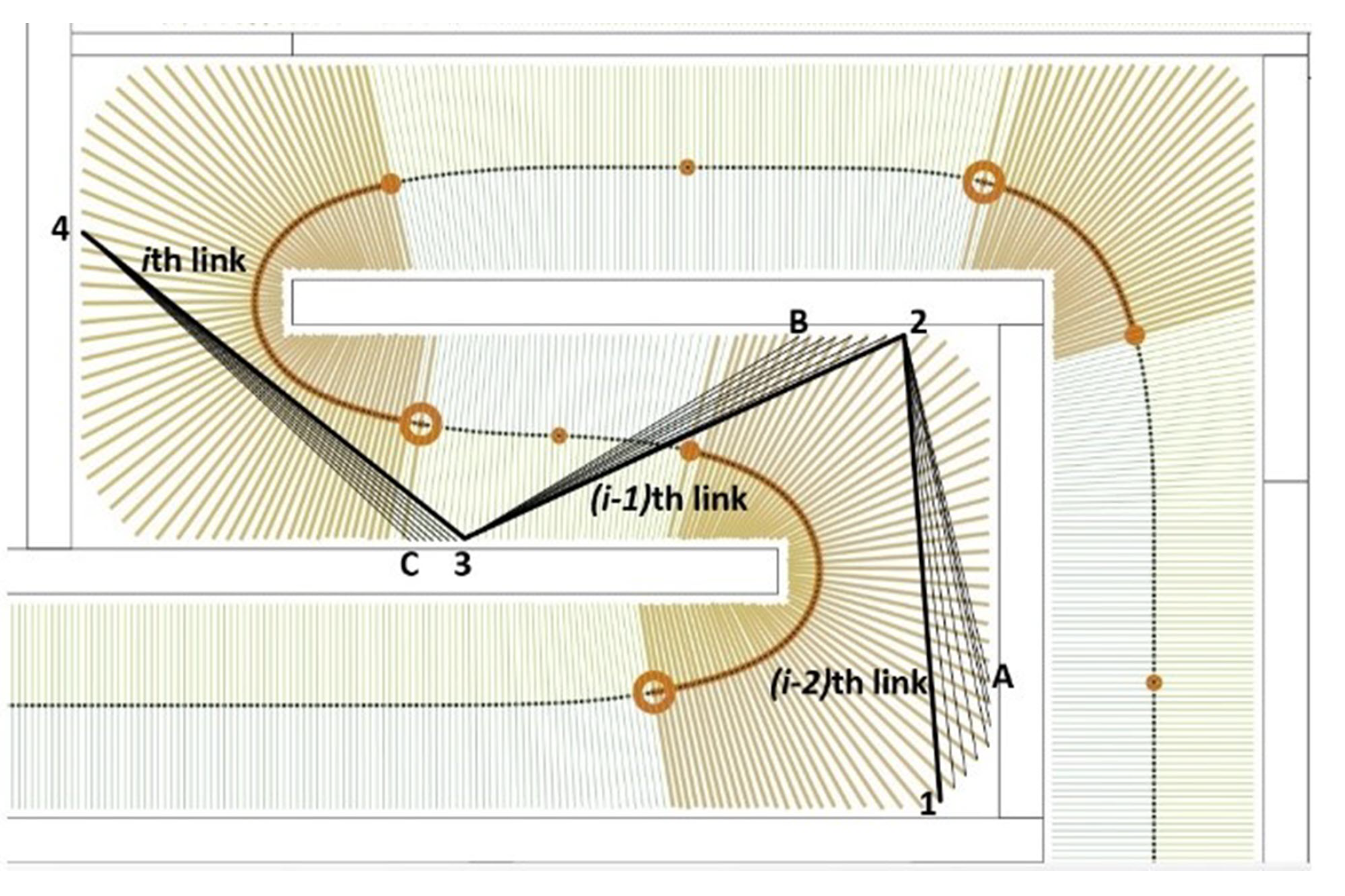
4.2. Determining Critical Regions

The right and the left beam lengths and their curvatures are obtained for each path point. Critical regions are formed from the path points whose right or left beam lengths are under a predefined magnitude and whose curvatures are above a predefined magnitude. For example, in Figure 7, there are three critical regions. The first critical region is the region numbered as 2 on the right starting from the point numbered as 1 and ending at the point numbered as 3. The second critical region is the one numbered as 8 on the left starting from the point numbered as 7 and ending at the point numbered as 9. The last critical region is the one numbered as 12 on the left starting from the point numbered as 11 and ending at the point numbered as 13.

Note that the unused beams are not drawn in the figure for the sake of clarity. The critical region numbered as 2 is on the right side while the next critical region numbered as 8 on the left side. To put it another way, these critical regions are in the opposite directions. Therefore, a direction change is mandatory here. This is one of the two crucial steps developing the algorithm. See Figure 7, the direction change occurs in the middle of the distance numbered as 5 between the two regions numbered as 4 and 6. Since the distance between the points 3 and 7 is very short with respect to the link length, the direction change should be at the midpoint of the distance numbered as 5. However, there are more than one point that works around the point 5. Another matter here is that switching from one array to another makes programming more difficult. Hence, the right array values are copied to the left array values or vice versa, which results in all the values being in a single array.

Recalling Figure 7, consider the second critical region numbered 8 and the third critical region numbered 12. Since they are both at the left side, no direction change is entailed at the point 10. The last direction change in the figure takes place at the point 14. One more thing: when the distance between critical regions is longer than the link length, the direction change occurs earlier, not in the middle of the distance. Again, it is possible to choose a direction change value out of possible several values.

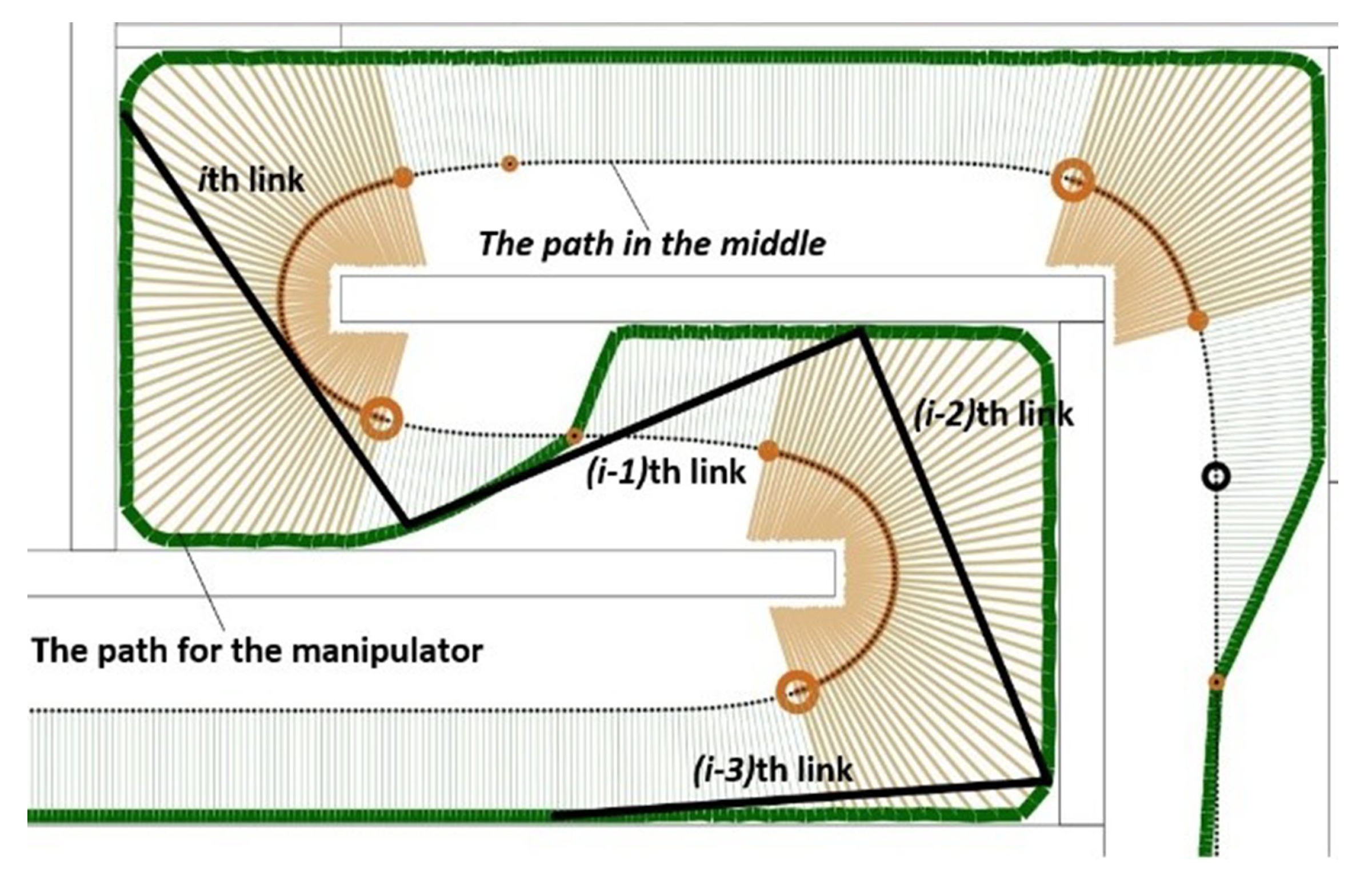
4.3. Determining the Path for the Manipulator

After determining critical regions and switching points, the path for the manipulator is obtained as shown in Figure 8 with thick green lines. In the same figure, there are also four manipulator links whose end points are mapped onto the path points are shown.

4.4. Control Strategy

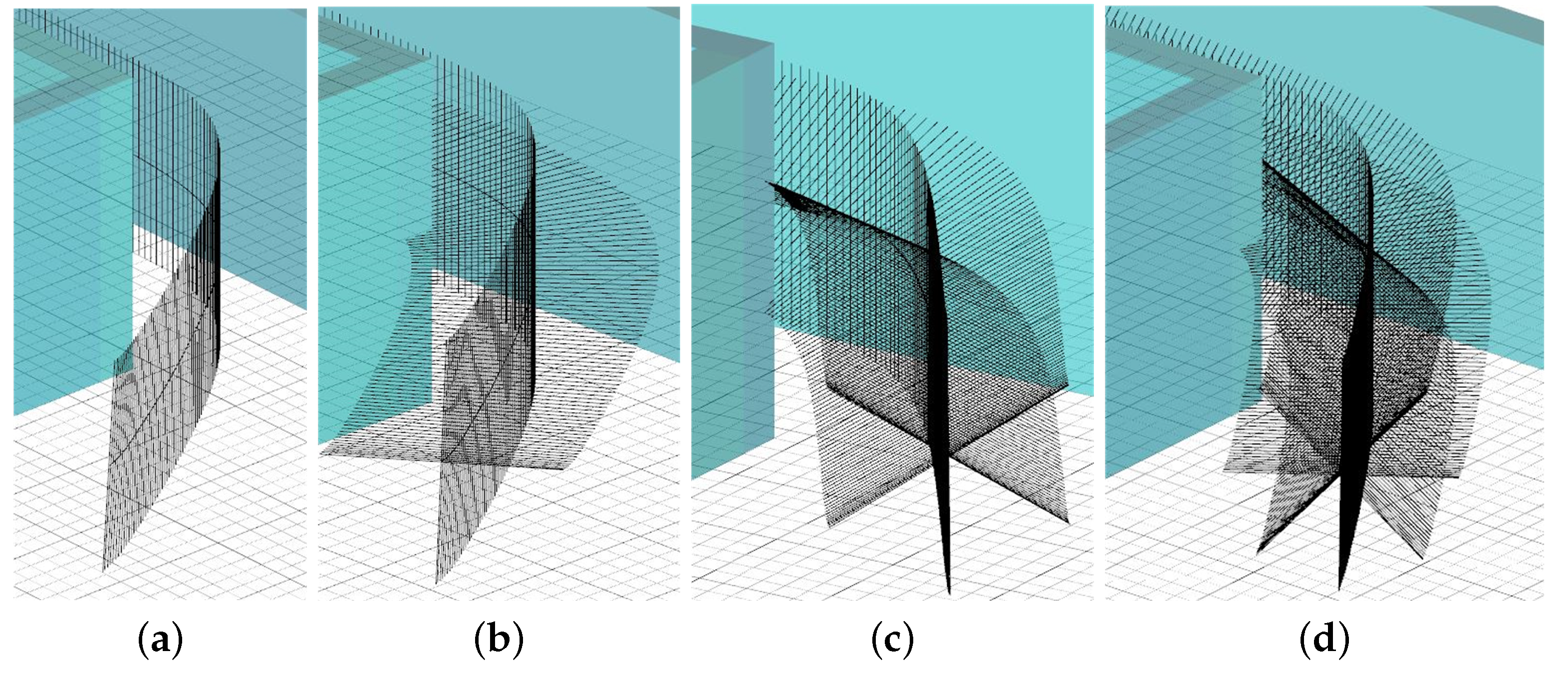
Since the proposed algorithm has a simple control strategy, it does not need a flowchart. All the work that is necessary for path planning has been prepared so far. The only thing left is to use this work in accordance with the statement below.

“While advancing the end-effector of the manipulator, keep each link’s end points on the path constructed from the left and right beams’ far ends until the end-effector reaches the goal.”

Keeping the end points of the links on the path is accomplished by means of a simple numerical procedure in real-time. Consider Figure 9, there are three successive links to be mapped on the curve. Suppose that the proximal end of ith link is moved to the point 4 on the path. The distal end of ith link is searched starting from the point C backward towards the point 3. When the distance between the point 4 and the point searched is approximately equal to the link length, the search is stopped and the link is mapped between these points. For the example given, the mapping is done between the points 4 and 3. In a similar manner, a search is performed for each link. In Figure 9, for (i −1)th and (i− 2)th links, searches are done from the point B to the point 2 and from the point A to the point 1 and new endpoints of these links are found at the points 2 and 1. Therefore the points that these three links are mapped onto the path are the ones 3, 2 and 1.

4.5. Beams in 3D

So far, all the work has been carried out in 2D workspace. When it comes to work in 3D space, the first task is to generate the potential field in 3D, then to find the middle path for a point robot from the start point to the goal point as seen in Figure 10.

Sending beams in 3D is not as easy as in 2D. The left and right beams in 2D cover all the free space which the robot moves within. On the other hand, sending just a couple of beams shown in Figure 11a barely covers the free space. Therefore, it cannot be used in 3D as in 2D. To cover the free space, it is possible to send beams in various directions at ${90}^{\circ }$ angles to the line tangent to the middle path. The more couples included, the more space is covered. In Figure 11, there are 1,2,3 and 4 couples shown. Although increasing the number of couples makes the resolution higher, not only it causes high computational costs but also it does not contribute to the maneuvering ability of the manipulator.

4.6. Determining Critical Areas and Switching Directions

As in 2D, using the points on the middle path, left and right beams’ coordinates are calculated for the first and second couples. Then, the critical points are determined using the same criterion applied in 2D case. In other words, all the critical areas are determined separately for each couple. For example, in Figure 12, the critical regions and three points between these critical regions are shown. In the figure, the first critical region’s last beam is shown with green sphere while the second critical region’s first beam is shown with blue sphere. The middle point between the points is shown with yellow sphere and the path points are shown with consecutive green points. These points are used to determine the switching points on the robot path. As can be seen from the figure direction switching occurs at the middle point which is shown with yellow sphere.

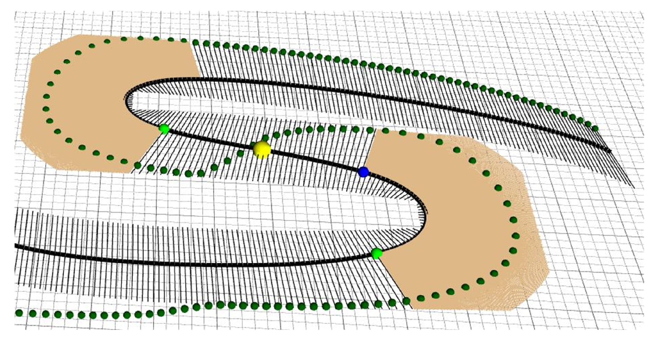
4.7. Determining Beam Couple Switching Points and the Manipulator Path

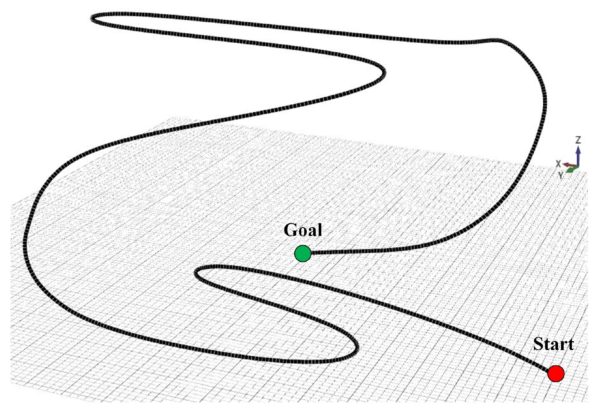
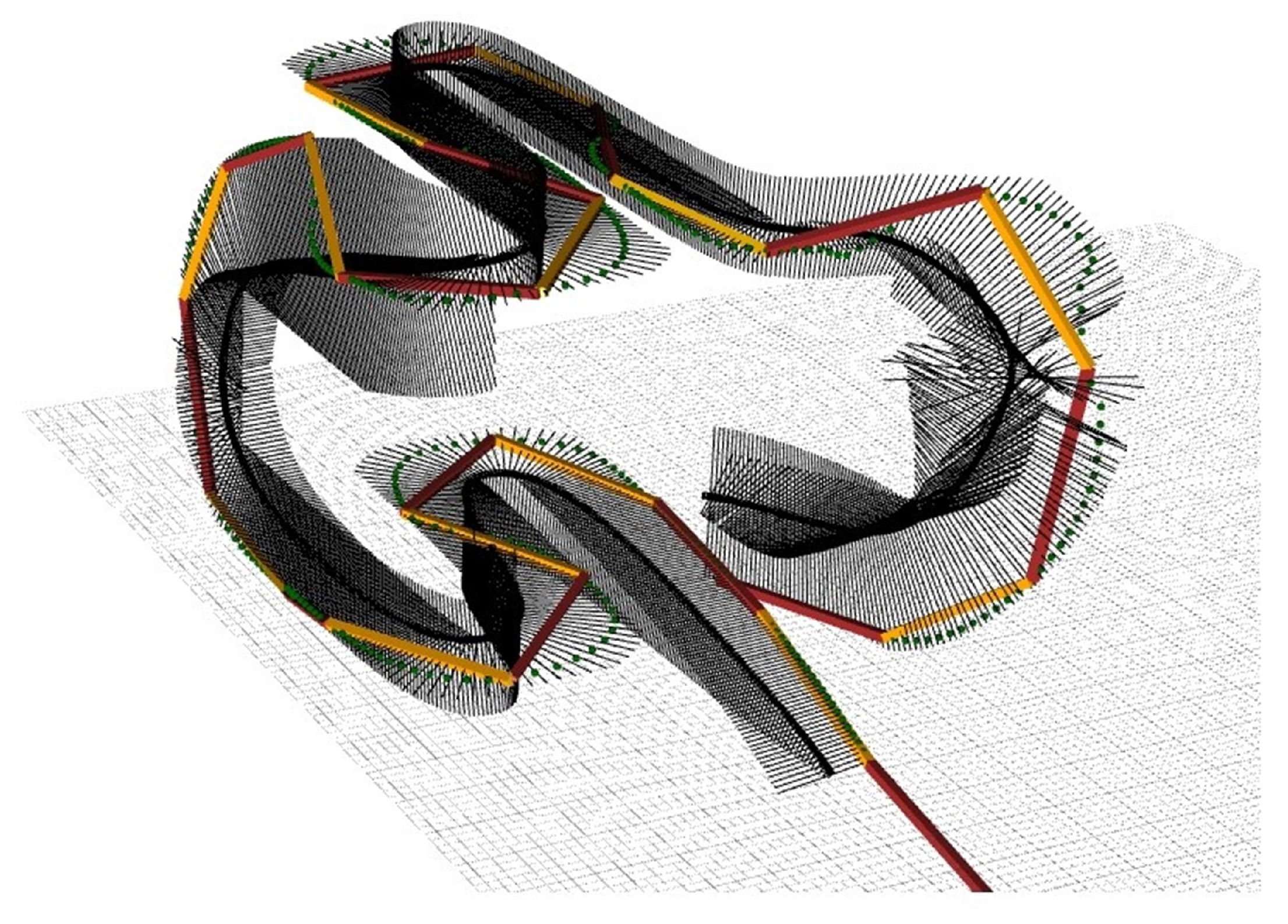
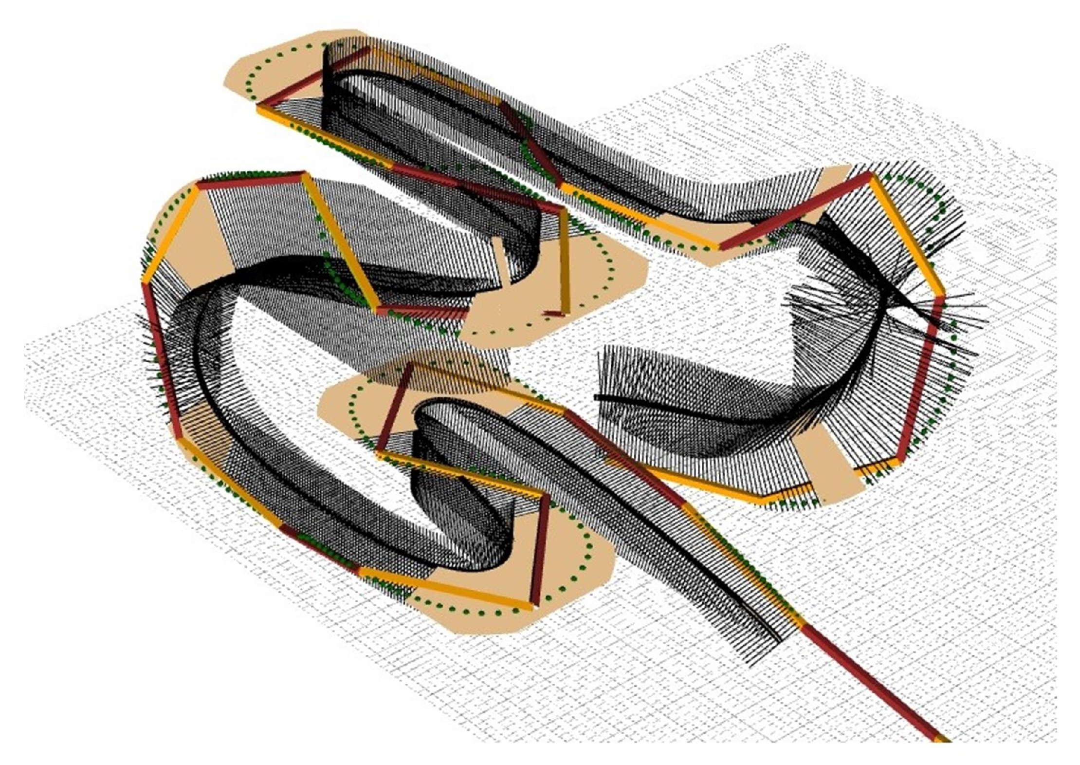
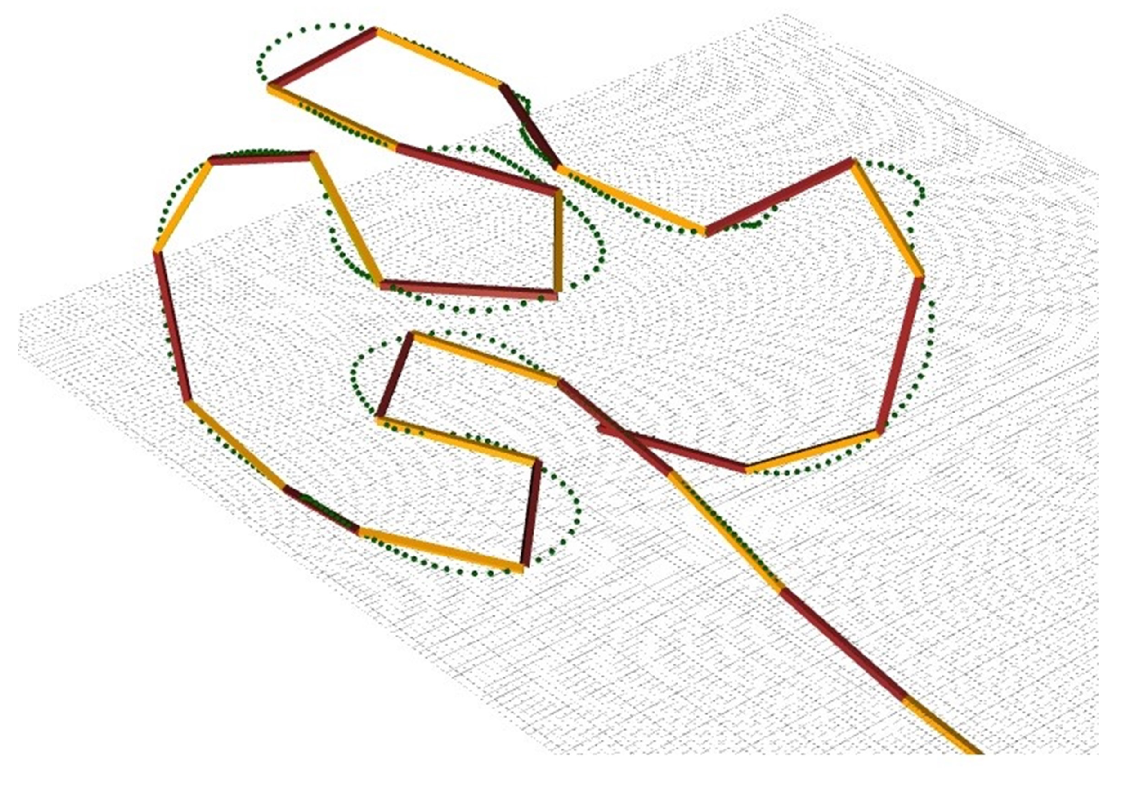
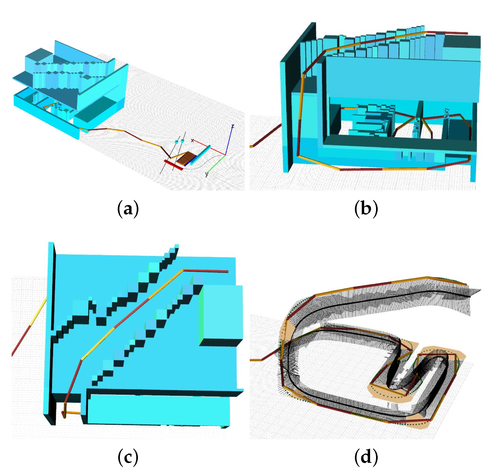
In the regions, one couple may have a critical region while another couple may not have. In such a situation, it is necessary to switch from one couple to another one. Note that this switching process is different from the switching process mentioned in Section 4.2 in such a way that previous switching process is implemented within only a couple while the switching process in this section is implemented between couples.

As seen in Figure 13, while the critical regions numbered as 1 and 2 belong to the first couple, the critical region numbered as 3 belongs to the second couple. The path points are shown with consecutive green points and the beam switching occurs at the point 9 which is the middle point of the end points numbered as 7 and 8 of successive critical regions.

Once the manipulator path is determined in 3D as described above, it is an easy process to move the end points of the manipulator links on the robot path points. Therefore, the manipulator navigates successfully in a 3D environment cluttered with many obstacles having tight maneuvering corners.

5. 3D Simulations

The computer program has been created in C# and executed on a laptop computer with United States of America (USA) Intel Corporation 6th Generation 2.60 GHz Core Processor called i7-6700HQ Central Process Unit (CPU) and 16 GB Random Access Memory (RAM). Graphics are managed with the Windows Presentation Foundation (WPF) development framework including Helix Toolkit which is available in a GitHub repository at https://github.com/helix-toolkit, accessed on 3 August 2022.

There are two examples given in this section. The first example is discussed in detail while the second is mentioned briefly for the sake of the paper length.

The workspace of the first example is shown in Figure 14 consisting of many different and narrow passages connected. Although the obstacles populated in the workspace consist of mainly rectangular-shaped obstacles rather than having various shapes, this arrangement represents the most difficult navigation strategies for the manipulator. In other words, if the manipulator navigates successfully through such obstacles, it is easy for the manipulator to navigate in the workspaces cluttered with many small and/or large obstacles. Actually, there is no significant difference for the potential fields to find a middle path between two types of workspaces.

At the place near to the origin of the workspace, there is a manipulator with 35 links placed on a mobile robot. There are also moving and stationary obstacles outside of the main obstacle structure, which is situated at the far side of the workspace.

As seen from Figure 15, the manipulator is carried to the front of its entrance on a mobile robot navigating through both moving and stationary obstacles.

Then, it starts to maneuver through obstacles. Note that only related part of the workspace is shown whenever suitable since the workspace is very large. Considering the workspace includes narrow passages in 3D, it is quite difficult to show the navigation process. That is why, some obstacles are hidden to show the manipulator motion through obstacles. Note that the snapshots of the manipulator navigating and auxiliary elements such as beams are taken from different angles in Figure 16. In the figure, it is seen that the manipulator has reached the goal point maneuvering through immensely narrow regions successfully in a 3D environment. To be able to help to visualize how the method works, some more figures are included. In Figure 17, the beam couples and manipulator path are shown.

In Figure 18, the critical regions are shown in addition to the ones shown in Figure 17.

In Figure 19, the manipulator path on which the ends of the links of the manipulator are kept while maneuvering is shown in green. The great efficiency of the method owes its success to this path.

For the example, the distance between two successive points on the path ($d_p$) is 16 pixels. It produces 6564 beams. The potential field is calculated in 13,022 milliseconds (ms) with 600 iterations. The reason for the high iteration number is actually the large workspace cluttered with so many obstacles. Because the potential field should be relaxed enough to realize the portions of the path away from the goal point. After having the path in the middle, calculations of the start and end coordinates of the beams are completed in 15,738 ms. The path for the manipulator is calculated in 117 ms, which is surprisingly short for a 3D environment. The manipulator reaches the goal in 14,623 ms. A simulation of the example is given without auxiliary elements in Video S1 and with auxiliary elements in Video S2.

The number of the beams affects navigation time. When $d_p$ value is taken as 8 pixels, the number of the beams becomes 13,128. The potential field is calculated in 13,280 ms with 600 iterations. After having the path in the middle, calculations of the start and end coordinates of the beams are completed in 32,500 ms, the path for the manipulator is calculated in 281 ms and navigation of the manipulator takes 30,251 ms.

As mentioned before, if the manipulator navigates successfully through such obstacles as in the first example, it is easy for the manipulator to navigate in the workspaces cluttered with many small and/or large obstacles. In order to show the proposed algorithm is a generalized algorithm, motion of the manipulator in a different environment which has small-sized obstacles is simulated.

The workspace of the second example is shown in Figure 20a. As seen from Figure 20b,c, the manipulator navigates through the obstacles and reaches the goal without any collision. Motion of the manipulator is given in Figure 20d without showing the obstacles. In addition, a simulation of the example is given without auxiliary elements in Video S3 and with auxiliary elements in Video S4 for the $d_p$ value of 16 pixels.

Potential field is calculated with 650 iterations in the second example. For two different value of the distance between two successive points on the path ($d_p$), number of the beams ($n_B$), calculation time of the potential field ($t_{PFC}$), calculation time of the beam couples ($t_{BC}$), calculation time of the manipulator path ($t_{MPC}$) and navigation time of the manipulator from the start to the goal point ($t_N$) are given for the both examples in

Table 1. Number of the beams and the calculation times of the proposed algorithm.

Example	${\mathit{d}}_{\mathit{p}}=8$ (pixels)					${\mathit{d}}_{\mathit{p}}=16$ (pixels)
	${\mathit{n}}_{\mathit{B}}$	${\mathit{t}}_{\mathit{PFC}}$(ms)	${\mathit{t}}_{\mathit{BC}}$(ms)	${\mathit{t}}_{\mathit{MPC}}$(ms)	${\mathit{t}}_{\mathit{N}}$(ms)	${\mathit{n}}_{\mathit{B}}$	${\mathit{t}}_{\mathit{PFC}}$(ms)	${\mathit{t}}_{\mathit{BC}}$(ms)	${\mathit{t}}_{\mathit{MPC}}$(ms)	${\mathit{t}}_{\mathit{N}}$(ms)
First	13,128	13,280	32,500	281	30,251	6564	13,022	15,738	117	14,623
Second	14,592	14,722	32,763	123	39,264	7296	13,822	15,124	56	29,578

.

6. Discussion and Future Work

In the benchmark environment shown in Figure 4, the lengths of $l_1$, $l_{link}$ and $l_{max}$ in pixels are 200, 350, and 440, respectively. It results in an index value of 0.8 for 3D environment. The maneuvering ability resulting in an index value of 0.8 means that it wastes almost no maneuvering space as long as it is physically attainable to maneuver.

As seen in Figure 21, if the middle path is followed or the manipulator links are mapped onto the middle path generated by the potential fields, the collision with obstacles are inevitable with the larger link lengths. In the proposed algorithm in this paper, this problem is solved by mapping the manipulator links onto a new path consisting of the end points of the beams in real-time.

The method is able to drive manipulators in a wide range: from few number of links to a huge number of links. The method’s complexities drive up almost linearly with the number of links.

The method is extensible since adding new features to the method has little influence on existing features consisting of a number of “if-else” statements. The method does not deal with the manipulator position using a kind of a propagation procedure between the links. On the contrary, the method in this paper handles the control in a simpler manner. It does not need to determine each link’s position by means of being tangent and it is capable of dealing with the tight maneuvering by reducing the control strategy to keeping the links’ end points on the manipulator path.

As mentioned before, the obstacles’ shapes are rectangular in the first example without tiny or different shaped obstacles scattered in the workspace. The crucial point to present in the paper is to show high maneuvering ability of the manipulator and the arrangement of the workspace with rectangular-shaped obstacles is the best to show this ability. However, in the second example small-sized obstacles are used.

One issue is shown in Figure 22a. Although the algorithm finds the middle path, the critical regions and the path for the manipulator perfectly well, there is no way that the manipulator passes through the obstacles. Since the piece of the middle path in that region is too short with respect to the link length. Figure 22b shows the subsequent configurations of the links trying to maneuver in vain, the collisions can be seen clearly. Recalling Figure 22a, there is actually large free space seen on the left-hand side of the middle path. If the middle path is modified to accommodate this space, collision-free navigation can be done easily.

The real-time method presented here is a very efficient and robust with respect to maneuvering in a tight workspace cluttered with many obstacles. Since the proposed method has special cases, it is not a complete method which means that being successful all the time if it is physically possible. As a future work, there is a need for further exploration to be able to have a complete algorithm. We think that we are very close to having a complete algorithm. Regarding redundant/hyper-redundant manipulators, existing navigation methods in the literature are quite limited when it comes to utilizing redundancy of the manipulator [9,10,11,18,19,20,22,24,25,29,34,35,37,38]. Since there are few or no quantitative values with respect to robot, obstacle and workspace dimensions, comparing methods are a bit difficult. However, inspecting visually the figures in the papers reveals that there is ample free space in the workspace among obstacles including robots having unnecessarily high number of links with relatively simple navigation tasks. As a result, navigating in such a workspace with so many short link lengths leads to inefficient use of resources, On the other hand, the method presented in our paper significantly increases maneuvering ability of redundant/hyper-redundant manipulators utilizing narrow spaces through obstacles by using fewer number of DOFs while being simple, robust and without restriction on the number of links used.

7. Conclusions

In this paper, a simple novel robust real-time algorithm is presented for path planning of redundant/hyper redundant manipulators within narrow terrains cluttered with obstacles in 3D environments. Using potential fields, a global path consisting of points in the middle of the free space from the start point to the goal point through obstacles is obtained. Having the path, two beam couples start from its path point and end at the obstacle border is generated. Critical regions consisting of critical corners that are formed from the path points whose beam couples satisfy certain criteria are obtained. Then, considering maneuvering direction of the manipulator for each critical region, path switching points on the same beam couple are determined as the middle point of the end point of the first critical region and the start point of the second critical region if the maneuvering direction changes between these consecutive critical regions. After determining critical regions and switching points for the selected beam couple, the beam switching points are determined considering the critical regions presence on both beam couples. Finally the path for the manipulator is obtained and the manipulator becomes ready to move. While advancing the end-effector of the manipulator, each link’s end points are kept on the path until the end-effector reaches the goal. Compared to navigation methods in the literature utilizing redundancy of hyper-redundant manipulators, it is seen that the method presented in our paper significantly increases maneuvering ability of redundant/hyper-redundant manipulators utilizing narrow spaces through obstacles by using fewer number of DOFs. The method is simple and robust. While it almost uses the minimum number of links physically required for the task, there is no restriction on the number of links used. The exemplary computer simulations with detailed figures embody the noticeable advantage of the proposed method while verifying the effectiveness of it.

References

1. Conkur, E.S.; Buckingham, R. Clarifying the definition of redundancy as used in robotics. Robotica 1997, 15, 583–586. [Google Scholar]
2. Chiacchio, P.; Chiaverini, S.; Sciavicco, L.; Sicilliano, B. Closed-loop inverse kinematics schemes for constrained redundant manipulators with task space augmentation and task priority strategy. Int. J. Robot. Res. 1991, 10, 410–425. [Google Scholar]
3. Nakamura, Y. Advanced Robotics: Redundancy and Optimization; Addison-Wesley Publishing Company: Boston, MA, USA, 1991; pp. 125–150. [Google Scholar]
4. Ma, S.; Hirose, S.; Yoshinada, H. Development of a hyper-redundant multijoint manipulator for maintenance of nuclear reactors. Adv. Robot. 1994, 9, 281–300. [Google Scholar]
5. Seereeram, S.; Wen, J.T. A global approach to path planning for redundant manipulators. IEEE Trans. Robot. Autom. 1995, 11, 152–160. [Google Scholar]
6. Schilling, R.J.; Read, R.; Lovass-nagy, V.; Walker, G. Path tracking with the links of a planar hyper-redundant robotic manipulator. J. Robot. Syst. 1995, 12, 189–197. [Google Scholar]
7. Takahashi, O.; Schilling, R.J. Motion planning in a plane using generalized Voronoi diagrams. IEEE Trans. Robot. Autom. 1989, 5, 143–150. [Google Scholar]
8. Khatib, O. Real-time obstacle avoidance for manipulators and mobile robots. In Proceedings of the IEEE International Conference on Robotics and Automation (ICRA), St. Louis, MO, USA, 25–28 March 1985; pp. 500–505. [Google Scholar]
9. Motahari, A.; Zohoor, H.; Korayem, M.H. A new obstacle avoidance method for discretely actuated hyper-redundant manipulators. Sci. Iranica B 2012, 19, 1081–1091. [Google Scholar]
10. Machmudah, A.; Parman, S.; Abbasi, A.; Solihin, M.I.; Manan, T.S.A.; Beddu, S.; Ahmad, A.; Rasdi, N.W. Cyclic path planning of hyper-redundant manipulator using whale optimization algorithm. Int. J. Adv. Comput. Sci. Appl. 2021, 12, 677–686. [Google Scholar]
11. Wei, H.; Zheng, Y.; Gu, G. RRT-based path planning for follow-the-leader motion of hyper-redundant manipulators. In Proceedings of the IEEE International Conference on Intelligent Robots and Systems (IROS), Prague, Czech Republic, 27 September–1 October 2021; pp. 3198–3204. [Google Scholar]
12. Latombe, J.C. Robot Motion Planning; Springer: Boston, MA, USA, 1991; pp. 54–104. [Google Scholar]
13. Conkur, E.S. Path following algorithm for highly redundant manipulators. Robot. Auton. Syst. 2003, 45, 1–22. [Google Scholar]
14. Tang, L.; Zhu, L.M.; Zhu, X.Y.; Gu, G. Confined spaces path following for cable-driven snake robots with prediction lookup and interpolation algorithms. Sci. China Technol. Sci. 2020, 63, 255–264. [Google Scholar]
15. Chirikjian, G.S.; Burdick, J.W. An obstacle avoidance algorithm for hyper-redundant manipulators. In Proceedings of the IEEE International Conference on Robotics and Automation (ICRA), Cincinnati, OH, USA, 13–18 May 1990; pp. 625–631. [Google Scholar]
16. Graham, A.; Buckingham, R. Real-time collision avoidance of manipulators with multiple redundancy. Mechatronics 1993, 3, 89–106. [Google Scholar]
17. McLean, A.; Cameron, S. Snake-based path planning for redundant manipulators. In Proceedings of the IEEE International Conference on Robotics and Automation (ICRA), Atlanta, GA, USA, 2–6 May 1993; pp. 275–282. [Google Scholar]
18. Wang, W.; Zhu, M.; Wang, X.; He, S.; He, J.; Xu, Z. An improved artificial potential field method of trajectory planning and obstacle avoidance for redundant manipulators. Int. J. Robot. Syst. 2018, 15, 1–13. [Google Scholar]
19. Lin, C.-C.; Chuang, J.-H. A potential-based path planning algorithm for hyper-redundant manipulators. J. Chin. Inst. Eng. 2010, 33, 415–427. [Google Scholar]
20. Fahimi, F.; Ashrafiuon; Nataraj, C. Obstacle avoidance for spatial hyper-redundant manipulators. In Proceedings of The First Asian Conference on Multibody Dynamics (ACMD), Iwaki, Fukushima, Japan, 31 July–2 August 2002; pp. 247–254. [Google Scholar]
21. Xidias, E.K.; Aspragathos, N.A. Time sub-optimal path planning for hyper redundant manipulators amidst narrow passages in 3D workspaces. In Advances on Theory and Practice of Robots and Manipulators, Mechanisms and Machine Science; Ceccarelli, M., Glazunov, V.A., Eds.; Springer: Cham, Switzerland, 2014; pp. 445–452. [Google Scholar]
22. Xidias, E.K. Time-optimal trajectory planning for hyper-redundant manipulators in 3D workspaces. Robot. Comput.-Integr. Manuf. 2018, 50, 286–298. [Google Scholar]
23. Choset, H.; Henning, W. A follow-the-leader approach to serpentine robot motion planning. J. Aerosp. Eng. 1999, 12, 65–73. [Google Scholar]
24. Ayten, K.K.; Sahinkaya, M.N.; Dumlu, A. Real time optimum trajectory generation for redundant/hyperredundant serial industrial manipulators. Int. J. Robot. Syst. 2017, 14, 1–14. [Google Scholar]
25. Ananthanarayanan, H.; Ordonez, R. A fast converging optimal technique applied to path planning of hyper-redundant manipulators. Mech. Mach. Theory 2017, 14, 231–246. [Google Scholar]
26. Reznik, D.; Lumelsky, V. Sensor-based motion planning in three dimensions for a highly redundant snake robot. Adv. Robot. 1994, 9, 255–280. [Google Scholar]
27. Azariadis, P.N.; Aspragathos, N.A. Obstacle representation by Bump-surfaces for optimal motion-planning. Robot. Auton. Syst. 2005, 51, 129–150. [Google Scholar]
28. Islam, M.N.; Tamura, S.; Murata, T.; Yanase, T. Evaluation of a new backtrack free path planning algorithm for manipulators. IEEJ Trans. Electron. Inf. Syst. 2008, 128, 1293–1302. [Google Scholar]
29. Chu, X.; Hu, Q.; Zhang, J. Path planning and collision avoidance for a multi-arm space maneuverable robot. IEEE Trans. Aerosp. Elect. Syst. 2018, 54, 217–232. [Google Scholar]
30. Miao, Y.; Gao, F.; Zhang, Y. Gait fitting for snake robots with binary actuators. Sci. China Technol. Sci. 2014, 57, 181–191. [Google Scholar]
31. Jamali, A.; Khan, M.R.; Osman, M.S.; Rahman, M.M.; Ashari, M.F.; Jamaludin, M.S.; Junaidi, E. Collision free control of variable length hyper redundant robot manipulator. Appl. Mech. Mater. 2014, 541–542, 1107–1114. [Google Scholar]
32. Collins, T.; Shen, W.M. PASO: An Integrated, Scalable PSO-Based Optimization Framework for Hyper-Redundant Manipulator Path Planning and Inverse Kinematics. Available online: https://www.isi.edu/division3/robots/prl/collins2016-ISI-TR-697.pdf (accessed on 17 July 2022).
33. Tappe, S.; Pohlmann, J.; Kotlarski, J.; Ortmaier, T. Towards a follow-the-leader control for a binary actuated hyper-redundant manipulator. In Proceedings of the IEEE/RSJ International Conference on Intelligent Robots and Systems (IROS), Hamburg, Germany, 28 September–2 October 2015; pp. 3195–3201. [Google Scholar]
34. Zheng, Y.; Wu, B.; Chen, Y.; Zeng, L.; Gu, G.; Zhu, X. Design and validation of cable-driven hyper-redundant manipulator with a closed-loop puller-follower controller. Mechatronics 2021, 78, 102605. [Google Scholar]
35. Tang, L.; Huang, J.; Zhu, L.-M.; Zhu, X.; Gu, G. Path tracking of a cable-driven snake robot with two-level motion planning method. IEEE/ASME Trans. Mechatronics 2019, 24, 935–946. [Google Scholar]
36. Tang, L.; Zhu, L.M.; Zhu, X.; Gu, G. A serpentine curve based motion planning method for cable-driven snake robots. In Proceedings of the 25th International Conference on Mechatronics and Machine Vision in Practice (M2VIP), Stuttgart, Germany, 20–22 November 2018; pp. 5–10. [Google Scholar]
37. Lin, Y.; Wang, J.; Xiao, X.; Qu, J.; Qin, F. A snake-inspired path planning algorithm based on reinforcement learning and self-motion for hyper-redundant manipulators. Int. J. Robot. Syst. 2022, 19, 1–13. [Google Scholar]
38. Xu, W.; Mu, Z.; Liu, T.; Liang, B. A modified modal method for solving the mission-oriented inverse kinematics of hyper-redundant space manipulators for on-orbit servicing. Acta Astronaut. 2017, 139, 54–66. [Google Scholar]
39. Jia, L.; Huang, Y.; Chen, T.; Guo, Y.; Yin, Y.; Chen, J. MDA + RRT: A general approach for resolving the problem of angle constraint for hyper-redundant manipulator. Exp. Syst. Appl. 2022, 193, 116379. [Google Scholar]
40. Qin, G.; Wu, H.; Cheng, Y.; Pan, H.; Zhao, W.; Shi, S.; Song, Y.; Ji, A. Adaptive trajectory control of an under-actuated snake robot. App. Math. Mod. 2022, 106, 756–769. [Google Scholar]
41. Duan, J.; Wang, B.; Cui, K.; Dai, Z. Path planning based on NURBS for hyper-redundant manipulator used in narrow space. Appl. Sci. 2022, 12, 1314. [Google Scholar]
42. Conkur, E.S.; Buckingham, R. Manoeuvring highly redundant manipulators. Robotica 1997, 15, 435–447. [Google Scholar]
43. Bulut, Y.; Conkur, E.S. A real-time path-planning algorithm with extremely tight maneuvering capabilities for hyper-redundant manipulators. Eng. Sci. Technol. Int. J. 2021, 24, 247–258. [Google Scholar]
44. Conkur, E.S.; Buckingham, R.; Harrison, A. The beam analysis algorithm for path planning for redundant manipulators. Mechatronics 2005, 15, 67–94. [Google Scholar]
45. Conkur, E.S. Path planning using potential fields for highly redundant manipulators. Robot. Auton. Syst. 2005, 52, 209–228. [Google Scholar]
Figure 1. The largest descent in 2D.
Applsci 12 08882 g001
Figure 2. Parameters needed for determining a path point in 3D environment.
Applsci 12 08882 g002
Figure 3. Interpolation in 3D environment.
Applsci 12 08882 g003
Figure 4. Benchmark environment.
Applsci 12 08882 g004
Figure 5. Global path generated in the middle of the workspace and basic definitions.
Applsci 12 08882 g005
Figure 6. Beam definitions.
Applsci 12 08882 g006
Figure 7. Path preparation definitions.
Applsci 12 08882 g007
Figure 8. Path generated for the manipulator.
Applsci 12 08882 g008
Figure 9. Mapping the manipulator onto its path.
Applsci 12 08882 g009
Figure 10. Generating potential field in 3D environment (Obstacles are not shown).
Applsci 12 08882 g010
Figure 11. Beam couples. (a) One couple. (b) Two couples. (c) Three couples. (d) Four couples.
Applsci 12 08882 g011
Figure 12. Critical regions and points for one beam couple.
Applsci 12 08882 g012
Figure 13. Critical regions and points for two beam couples.
Applsci 12 08882 g013
Figure 14. Workspace for the first example.
Applsci 12 08882 g014
Figure 15. Manipulator maneuvering through obstacles on a mobile robot.
Applsci 12 08882 g015
Figure 16. Snapshots of the manipulator motion from different angles. (a) Start of the motion. (b) Switching beam couple. (c) Tight maneuvering with auxiliary elements. (d) Tight maneuvering without auxiliary elements. (e) Reaching the goal while tight maneuvering. (f) End of the motion.
Applsci 12 08882 g016
Figure 17. Beam couples and manipulator path.
Applsci 12 08882 g017
Figure 18. Critical regions.
Applsci 12 08882 g018
Figure 19. Tight maneuvering in 3D environment.
Applsci 12 08882 g019
Figure 20. Tight maneuvering in the second example. (a) General view of the workspace and start of the motion. (b) Tight maneuvering. (c) Reaching the goal. (d) The whole part and auxiliary elements (Obstacles are not shown).
Applsci 12 08882 g020
Figure 21. Collision with obstacles when manipulator is following the middle path.
Applsci 12 08882 g021
Figure 22. (a) Special case. (b) Subsequent configurations of the links.
Applsci 12 08882 g022