A Classification Feature Optimization Method for Remote Sensing Imagery Based on Fisher Score and mRMR

Abstract

In object-oriented remote sensing image classification experiments, the dimension of the feature space is often high, leading to the “dimension disaster”. If a reasonable feature selection method is adopted, the classification efficiency and accuracy of the classifier can be improved. In this study, we took GF-2 remote sensing imagery as the research object and proposed a feature dimension reduction algorithm combining the Fisher Score and the minimum redundancy maximum relevance (mRMR) feature selection method. First, the Fisher Score was used to construct a feature index importance ranking, following which the mRMR algorithm was used to select the features with the maximum correlation and minimum redundancy between categories. The feature set was optimized using this method, and remote sensing images were automatically classified based on the optimized feature subset. Experimental analysis demonstrates that, compared with the traditional mRMR, Fisher Score, and ReliefF methods, the proposed Fisher Score–mRMR (Fm) method provides higher accuracy in remote sensing image classification. In terms of classification accuracy, the accuracy of the Fm feature selection method with RT and KNN classifiers is improved compared with that of single feature selection method, reaching 95.18% and 96.14%, respectively, and the kappa coefficient reaches 0.939 and 0.951, respectively.

1. Introduction

The spectra, textures, and geometry of high-resolution remote sensing images are very rich, and different features describe ground objects from different angles [1,2]. To give full play to the advantages of the spectral, texture, and geometric features of high-resolution remote sensing images, object-oriented classification usually allows more features to participate in classification. If all features participate in classification, the processing speed is greatly reduced, while the classification accuracy is reduced in the case of limited training samples [3,4]. Therefore, how to select the optimal features from the feature space to participate in classification is the primary problem to be solved in the field of high-resolution image object-oriented classification [5,6]. Feature selection is an important task in data mining and machine learning and can effectively reduce the dimension of data and improve the performance of algorithms [7,8]. With the increase in data, feature selection has become an indispensable part of data processing [9]. The purpose of feature selection is to remove irrelevant or redundant features, retain useful features, and obtain appropriate feature subsets [10]. Feature selection methods can be divided into three series: filter, wrapper, and embedded [11]. Among them, filter methods directly evaluate the statistical performance of all the training data, as this is independent of the subsequent learning algorithm. Although it has the advantage of fast speed, it has a large performance deviation from the subsequent learning algorithm and is not effective when considering big data features [12]. Wrapper methods evaluate a subset of features with respect to the training accuracy of the subsequent learning algorithm and have the advantage of small deviation, but this type of method is large in size and involves significant computational burden [13]. Embedded methods combine the advantages of the above methods to some extent, but the difficulty with this type of method is the need to construct a suitable function optimization model [14].

From the above analysis, it is clear that the various types of methods have limitations in feature selection. In order to address these limitations, we selected the Fisher Score [15,16] and mRMR [17] as filter methods for comparison with decision tree [18,19] and random forest methods, respectively. The RF [20,21], k-nearest neighbors (kNN) and support vector machine (SVM) approaches were combined for image classification. Filter methods can be divided into unsupervised, semi-supervised, and supervised feature selection methods [22,23]. At present, supervised feature selection methods include Relief-F [24], mRMR, and Fisher Score. The Relief-F algorithm is a typical filtered feature optimization algorithm, which calculates the weights of feature variables, ranks them, and then extracts the optimal set of features. The Relief-F algorithm is highly efficient and suitable for most data. The mRMR algorithm is a feature optimization method based on mutual information theory, which is used to maximize the correlation between a selected feature subset and the category, while ensuring that the redundancy between the selected features is as small as possible [25,26]. The Fisher Score is an effective criterion for judging the sample features, derived from Fisher’s linear discriminant, which finds feature subsets in the feature set space that maximize the distance between different categories of data points while minimizing the distance between those in the same category. Based on the above, we chose to combine the Fisher Score and mRMR algorithm to downscale the feature space of remote sensing images, where the Fisher Score is used to calculate the ratio of the variance within each feature class and the variance between each feature class, while the mRMR algorithm is used to filter out those features with the greatest relevance to the target category and the least redundancy between them. Finally, the filtered features are used as feature subsets. In this study, the feature dimension of the remote sensing image was reduced by combining two feature selection methods, and the optimal feature subset was obtained through feature dimension reduction, which can reduce the classification time of classifier and improve the classification accuracy of the image. We also selected different types of feature selection methods to verify the ability of the Fm feature dimensionality reduction. In addition, we utilized a variety of classifiers and selected the one suitable for Fm by comparing their overall classification accuracy.

2. The Study Area and the Data Source

2.1. Study Area

The study area is located in Guang’an area, Sichuan Province, China, between 106°38′–106°41′ E and 30°27′–30°29′ N. According to a ground cover map of the study area, the ground objects in this area can be classified as water, vegetation, bare ground, buildings, and roads. The location of the study area is shown in Figure 1.

2.2. Data Source and Preprocessing

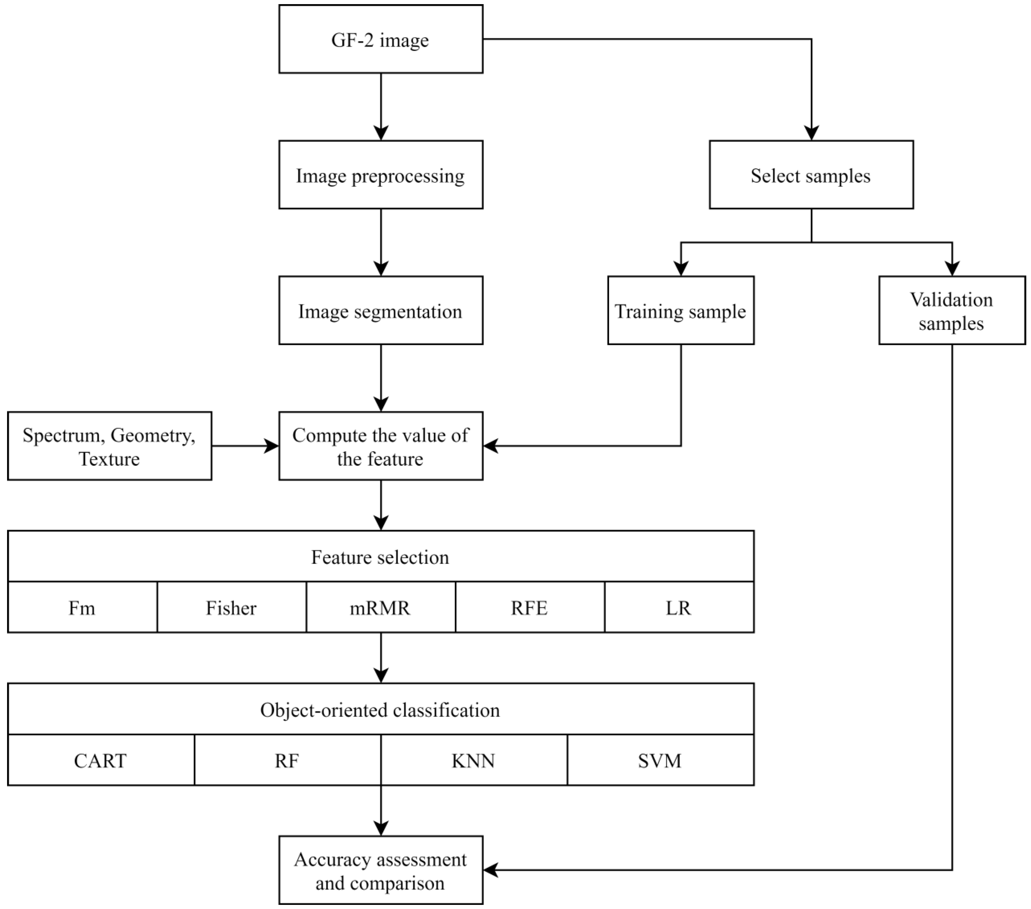
The data came from the China Centre for Resources Satellite Data and Application (https://data.cresda.cn/#/home, accessed on 10 January 2022). The data used were multi-spectral and panchromatic ortho-corrected images obtained by the GF-2 satellite in August 2020, including multi-spectral data at 4 m resolution (four bands of red, green, blue and near-red) and panchromatic data at 1 m resolution [27]. Radiation calibration, atmospheric correction, geometric rectification, and alignment were performed on the CF-2 images using the ENVI software, while the NNDiffuse Pan-Sharpening fusion algorithm was used to generate multi-spectral remote sensing data with 1 m resolution.

3. Research Methods

Object-oriented classification methods based on feature selection mainly include the steps of image pre-processing, multi-scale segmentation, construction of initial feature space, and image classification. The technical process is depicted in Figure 2. Firstly, the image data were preprocessed based on ENVI5.3. The detailed preprocessing process is shown in Section 2.2. Secondly, eCognition9.0 was used to segment the image, and then some objects were selected as training samples to calculate the eigenvalues of spectral, texture and geometric features of each sample. Third, based on PyCharm software, five feature selection methods were used to screen out feature subsets. Finally, four machine learning classifiers were used to train the training samples and classify the images. The accuracy of the classified remote sensing images was evaluated using validation samples.

3.1. Build the Feature Space

Based on the ground object types in the study area as well as empirical knowledge, the initial feature space constructed in this study contained 32 features. Spectral features included the mean and standard deviation in bands 1–4 of the GF-2 images; geometric features included the area, length, and width of objects; and texture features included homogeneity, contrast, heterogeneity, angular second moment, entropy, and the correlation between the gray-level co-occurrence matrix (GLCM) and gray-level difference vector (GLDV). The feature information is shown in

Table 1. Feature information.

Feature Type	Feature Name	Number of Features
Spectrum	Mean value of bands 1–4, Standard deviation of bands 1–4, Brightness, Max. diff, NDVI, NDWI	12
Geometry	Area, Length, Width, Length/Width, Density, Compactness, Border length, Number of pixels	8
Texture	Homogeneity, Contrast, Dissimilarity, Ang. 2nd moment, Entropy, Correlation, StdDev, Mean	12

.

3.2. Feature Selection

There are many kinds of image features. Choosing appropriate features can improve the accuracy and efficiency of object-oriented automatic classification. The principle of feature selection is to reduce the total quantity of data while not reducing the classification-related information by obtaining a small subset of features to achieve the purpose of feature optimization.

(1) Fisher Score feature weight calculation. The Fisher Score provides an effective method for feature selection, which mainly identifies features with strong performance. When it is as small as possible within a class and as large as possible between classes, the optimal feature subset can be selected [28,29,30]. Let the inter-class variance of the k^th feature in the data set be expressed by $S_B^{(k)}$. Then, the calculation formula is shown in Equation (1) [28,29].

$$S_B^{\left(k\right)}={\displaystyle \sum }_{i=1}^c\frac{n_i}{n}{(m_i^{\left(k\right)}-m^{\left(k\right)})}^2$$

(1)

where $c$ denotes the number of sample classes, $n$ denotes the total number of samples, $n_i$ denotes the number of samples in the ith class of the sample, $m_i^{(k)}$ denotes the mean of the values taken by the samples in the ith class on the kth feature, and $m^{(k)}$ denotes the mean of the values taken by the samples in all classes on the kth feature. Let the intra-class variance of the kth feature on the data set be denoted by $n_i$. Then, the formula is shown in Equation (2) [28,29]:

$$S_w^{\left(k\right)}=\frac{1}{n}{\displaystyle \sum }_{i=1}^C{\displaystyle \sum }_{x\in w_i}{(x^{\left(k\right)}-m_i^{\left(k\right)})}^2$$

(2)

where $x^{(k)}$ denotes the value of sample $x$ on the kth feature and $w_i$ denotes the ith class sample. The weight coefficient of the kth feature on the data set is denoted by $J_{fisher}(k)$. The calculation formula is shown in Equation (3) [28,30]:

$$J_{fisher}\left(k\right)=\frac{S_B^{\left(k\right)}}{S_w^{\left(k\right)}}$$

(3)

(2) mRMR filtering feature subset. The mRMR algorithm is a heuristic feature selection algorithm which calculates the correlation between features and attributes based on an evaluation function, ranks the original features, and obtains a feature set with high correlation and few redundant features [31,32,33].

The mutual information [34] is first calculated in order to determine the correlations between features and between features and categories. The mutual information formula for variables $M$ and $N$ is [32]:

$$I\left(M;N\right)={\displaystyle \sum }_{m\in M}{\displaystyle \sum }_{n\in N}p\left(m,n\right)log\frac{p\left(m,n\right)}{p\left(m\right)p\left(n\right)}$$

(4)

where $p(m)$ and $p(n)$ denote the probability density functions of the random variables m and n, and $p(m,n)$ denotes the joint probability density function of the random variables m and n. The greater the mutual information, the greater the correlation between $M$ and $N$. A feature subset $S$ containing K features is searched to maximize the correlation between the K features and a category $c$. The maximum correlation is calculated as shown in Equation (5) [31,32]:

$$maxD\left(S,c\right),D=\frac{1}{\left|S\right|}{\displaystyle \sum }_{x_i\in S}I\left(x_i;c\right)$$

(5)

The correlation between feature set $S$ and class $c$ is determined by the average of all mutual information values between each feature $x_i$ and class $c$, and $k$ sets with maximum average mutual information are selected. Subsequently, the redundancy between the $k$ features is eliminated, where the minimum redundancy is calculated as shown in Equation (6) [31,32]:

$$minR\left(S\right),R=\frac{1}{{\left|S\right|}^2}{\displaystyle \sum }_{x_i,x_j\in S}I\left(x_i,x_j\right)$$

(6)

The maximum correlation and minimum redundancy are combined to form the mRMR algorithm, and the formula for calculating $D$ and $R$ using the operator $\mathsf{\Phi }(D,R)$ is shown in Equation (7) [17,31]:

$$max\mathsf{\Phi }\left(D,R\right),\mathsf{\Phi }=D-R$$

(7)

Using this feature selection criterion, the features are selected by maximizing the defined operator $\mathsf{\Phi }()$, using an incremental search method. Based on the feature subset $S_{k-1}$, the k^th feature is calculated from the remaining feature space $X-S_{k-1}$, which is made to maximize $\mathsf{\Phi }()$ using the following equation, that is, the incremental feature selection optimization formula [17,31]:

$$\underset{x_j\in X-S_{k-1}}{max}\left[I\left(x_j;c\right)-\frac{1}{k-1}{\displaystyle \sum }_{x_i\in S_{k-1}}I\left(x_j;x_i\right)\right]$$

(8)

The weight of each feature is calculated according to the Fisher Score, and features with higher weight have better classification ability. As the correlation between features is not calculated, redundant features cannot be removed. However, the mRMR algorithm can obtain the feature subset that has the maximum correlation with the target category and the least redundancy, but it cannot obtain the weight coefficient of each feature, and the extracted feature subset cannot reflect the difference of the effect of different features on the classification.

Firstly, the Fisher Score calculation method was used to build the ranking rules of feature index importance, and the features with larger weight were selected by calculating the weight value of each feature. The feature vector with a high weight can be used as the dominant vector of the classification set, and the feature vector with a low weight has less influence on the classification result. Then, the mRMR algorithm was used to calculate the selected features, and the features with the maximum correlation and the minimum redundancy between the categories were selected. Therefore, by combining the Fisher Score and mRMR algorithms for feature dimension reduction, an optimal feature subset can be obtained.

In addition to the above two methods, in order to verify the reliability in the experiment, the commonly used recursive feature elimination (RFE) algorithm (a wrapped feature selection method) and logistic regression (LR) algorithm (an embedded feature selection method) were selected.

(3) RFE is a greedy algorithm [35]. It takes the whole data set as the starting point of the search and uses a feature ordering approach to select backward sequences from the whole set, eliminating one feature with the lowest ranking each time, until the feature subset that is most important for the classification results is selected. In the iterative process of the above steps, the order in which features are eliminated depends on their importance. The RFE algorithm requires a suitable classifier for modeling and prediction, for which the linear regression model was used in our experiment.

(4) LR is a machine learning model with simple form and good interpretability [36]. The LR model studies the multiple regression relationship formed between one dependent variable and multiple independent variables. Assuming a vector $x=(x_1,x_2,\dots ,x_n)$ of $n$ independent variables, representing $n$ characteristics of each sample, and letting the conditional probability $p(y=1|x)=p$ be the probability of occurrence of an event $x$ relative to an observed quantity, the LR model [36] can be expressed as

$$p\left(y=1|x\right)=\frac{1}{1+e^{-g\left(x\right)}}$$

(9)

where $g(x)=w_0+w_1{x}_1+\dots +w_n{x}_n$, $w_0,w_1,\dots ,w_n$ are the weights estimated with maximum likelihood.

3.3. Image Classification

In the classification process, the choice of classifier is an important factor determining the classification results. The CART decision tree, RF, k-nearest neighbors (kNN), and support vector machine (SVM) methods comprise four different classification algorithms.

The basic principle of CART is to form the test variables and the target variables into a data set, select the optimal segmentation features by calculating the Gini coefficient, then build a binary tree according to the feature values. These steps are cycled until the sample set to be classified reaches a stopping condition. There are two conditions for stopping: One is that there are no more feature variables for the target classification, and the other is that all samples of a given node belong to the same class. If the sample points of the stop classification node are of multiple classes, the node is specified as the class with the highest number of subclasses, and a new leaf is created within that class [37]. The binomial tree structure of the CART decision tree greatly improves the operational efficiency compared to the multinomial tree structure of the traditional decision tree [38].

The RF algorithm is an integrated classifier based on multiple decision trees. Through a bootstrap sampling method, a subset of samples is randomly selected from the original data as training samples, and decision trees are constructed for each training sample separately. A randomly selected feature is used as a node ($m$ < $N$) of the decision tree, which is split and grown based on the amount of feature information. The training process is iterated until the maximum tree depth set by the user is reached or the splitting cannot continue [39]. An RF consists of $N$ decision trees, and voting is used for each decision tree to obtain the final classification result [40]. RF has the advantage of high prediction accuracy, coupled with the fact that it is less prone to overfitting. Therefore, it has been widely used for image classification in high-resolution remote sensing data sets.

The kNN classification algorithm is a relatively simple machine learning algorithm [41]. In remote sensing image classification, this method determines the nearest k neighbors by calculating the distance between the samples to be classified and the training samples, then judges according to the categories of these k neighbors selected. The category to which the k neighbors belong the most is selected, and the samples to be classified are considered to belong to this category.

The SVM is a new machine learning method developed on the basis of statistical learning theory [42,43]. It is a non-parametric classifier. Based on the structural risk minimization criterion, the SVM solves image classification and regression problems by finding the optimal classification hyperplane in the high-dimensional feature space. According to the limited sample information, the best compromise between learning accuracy and learning effect can be obtained. The support vector machine has the advantages of simple implementation and high operational efficiency.

The above four classification algorithms each have their own advantages. In this study, all four algorithms are used to classify the optimized feature combination and the unoptimized full feature combination.

4. Object-Oriented Classification Process

The image segmentation in this study used the multi-scale segmentation [44] algorithm, where the segmentation parameters were determined by control variates. The basic principle of the control variates method is that all other parameters are unchanged, while only one of them is adjusted, and the best segmentation parameter combination is determined by adjusting the parameter values until each segmentation parameter is determined. Firstly, the shape factor and compactness factor are set as a fixed value, and then different segmentation scale parameters are set. The smaller the segmentation scale parameter, the larger the segmentation degree, and the more objects after segmentation. When the segmentation parameter is large, the image is undersegmented, and several ground objects are segmented into one object. After comparison, we found that when the segmentation scale is 80, the segmentation result is the best, and all different ground objects are divided. The size of shape factor and compactness factor also affect the segmentation result. A small form factor leads to poor segmentation of results, while a large form factor leads to excessively fragmented results. The compactness factor uses the shape criterion to optimize the results of the affected objects considering the overall compactness. When the shape factor is set to 0.1 and the compactness factor is set to 0.5, the segmentation effect of the experimental study area is better. After experimental analysis, when the segmentation scale, shape factor, and compactness factor were 80, 0.1, and 0.5, respectively, a relatively good segmentation effect was obtained, as depicted in Figure 3.

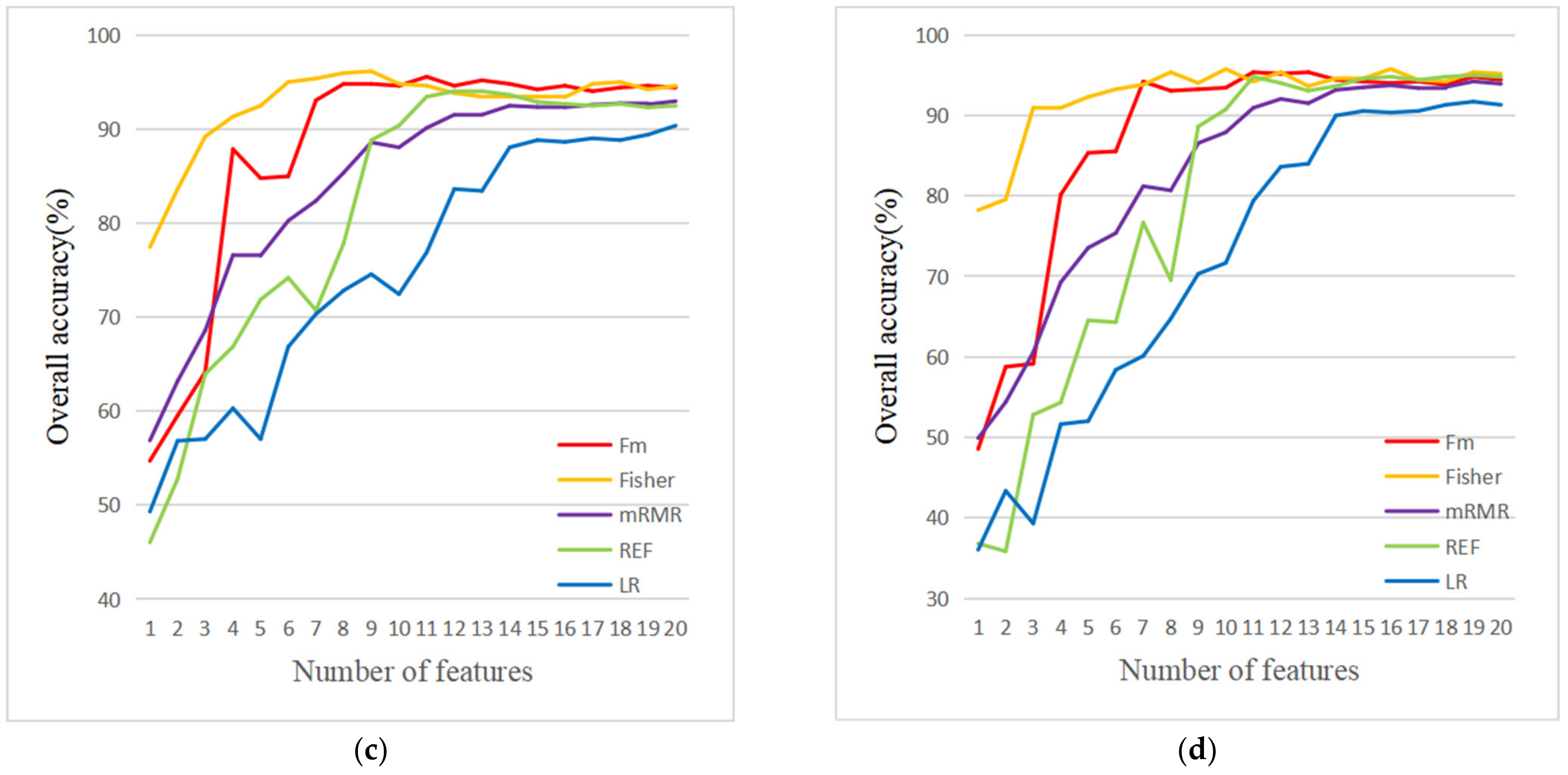
4.1. Feature Selection Results

As the classification results of image classification are influenced by the number of samples and spatial location, stratified random sampling was adopted for each category of features, such that the number of samples in each category was proportional to the total area of the category. We selected 2/3 of the segmented objects to extract the features, including texture, geometric, and spectral feature values, while the remaining samples were used for accuracy testing.

To explore the importance ranking of the relevant features, the top 15 features obtained with the five feature selection methods are listed in

Table 2. Top 15 features using various FS methods.

Fm	Fisher	mRMR	REF	LR
Standard_G	NDVI	Standard_R	GLCM_Entropy	GLCM_Ang_2nd moment
Density	NDWI	NDVI	Compactness	GLCM_Correlation
Standard_R	Mean_NIR	Length/Width	Standard_B	NDWI
Mean_B	Mean_B	GLCM_StdDev	Standard_R	Width
Width_Pxl	Area_Pxl	Standard_G	LengthWidt	GLCM_Mean
Border_length	Standard_B	Density	GLCM_StdDev	length
NDVI	Standard_NIR	Compactness	GLCM_Dissimilarity	GLDV_Entropy
Max_diff	Max_diff	GLCM_Correlation	GLCM_Mean_	GLCM_Homogeneity
GLDV_Entropy	Mean_R	GLCM_Dissimilarity	Mean_B	GLCM_StdDev
Standard_B	Width	Mean_B	Mean_G	Density
NDWI	Mean_G	Width_Pxl	Mean_NIR	max_diff
Mean_NIR	GLCM_Homogeneity	NDWI	Mean_R	Standard_NIR
GLDV_Ang_2nd moment	Standard_G	Number_of_	Standard_G	Length/Width
Mean_R	GLCM_Ang_2nd moment	Standard_B	GLDV_Entropy	NDVI
GLCM_Homogeneity	Brightness	GLCM_Mean	Standard_NIR	Standard_G

, while the proportions of different types of features in different subsets are shown in

Table 3. Summary of the characteristics in the different categories of the top 15 characteristics according to Table 2.

Feature Selection Method	Feature Description	Spectral	Geometric	Texture
Fm	Number of features	9	3	3
	Top 15 feature ratios	60.00%	20.00%	20.00%
Fisher	Number of features	11	2	2
	Top 16 feature ratios	73.33%	13.33%	13.33%
mRMR	Number of features	7	5	4
	Top 17 feature ratios	46.67%	33.33%	26.67%
REF	Number of features	8	2	5
	Top 18 feature ratios	53.33%	13.33%	33.33%
LR	Number of features	5	4	6
	Top 19 feature ratios	33.33%	26.67%	40.00%

. The results show that the features screened by different feature selection methods presented significant differences. In general, spectral and texture features accounted for a large proportion of the top 15 features. Figure 4 shows the correlation coefficient matrix of the top 15 features of different feature selection methods. The darker the grid color, the smaller the correlation coefficient between the features, and the more negative the correlation between the two features. On the contrary, the larger the correlation coefficient between features, the more positive the correlation between the two features.

Overall, the spectral features appeared significantly more frequently than the geometric and texture features. In the filtered feature selection method, NDVI, NDWI, Mean_B, Standard_B, Standard_G, and Width features were all present, while the number of texture features was more than 1/3. The mRMR and RFE algorithms selected seven features among the first 15 features which were the same, showing strong consistency. In addition, the LR algorithm appeared to choose more geometric and texture features, reaching 50% of the features in each category.

From the feature extraction results, it can be seen that spectral features were the most numerous. From the remote sensing images of the research area, the vegetation and water areas were larger than other land features, and NDVI and NDWI can effectively extract vegetation and water bodies. Secondly, there were many geometric features. Ground objects are usually characterized by large area and complex spectral features. It is difficult to distinguish objects such as roads and construction land from other ground objects only using spectral features, but they can be effectively classified using geometric features.

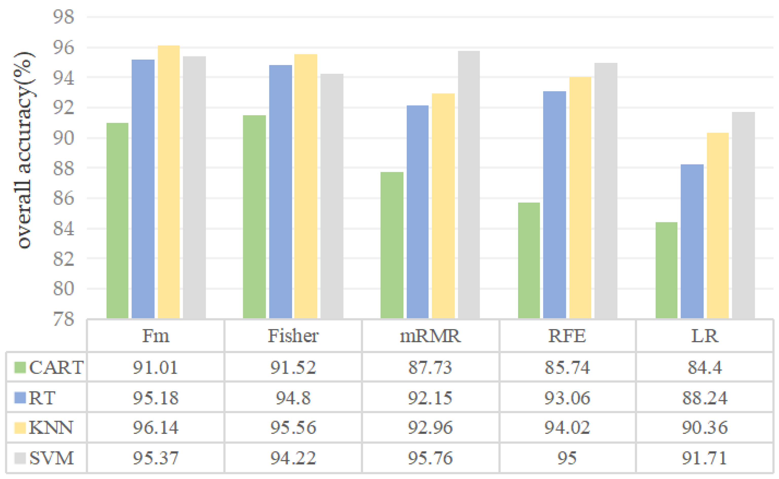
4.2. Comparison of Classification Results

As shown in Figure 5 below, based on the four classification methods, the trend of overall accuracy was obtained by continuously increasing the number of feature fields, and the feature selection methods were compared. As the number of features increased, the overall accuracy gradually improved. When the number of features reached about 15, the classification accuracy decreased slightly with an increase in the number of features, then remained stable. Therefore, in the process of object-oriented classification experiments, when too many features are involved in the classification, it may not be possible to achieve the optimal classification results, and instead the classification accuracy and classification efficiency are reduced. Overall, filtered feature selection methods presented better results than wrapped methods, while embedded feature selection methods presented the worst results. Furthermore, the SVM classification results were relatively stable, and the impact of different feature selection methods on the classification accuracy was smaller than the use of other classification methods.

According to Figure 6, the proposed Fm was found to have higher overall accuracy than the other feature selection methods with both RF and kNN classifiers, with accuracies of 95.18% and 96.14%, respectively. Although it was not optimal with the CART and SVM classifiers, the overall accuracy still achieved good results. This indicates that the combined scheme of Fisher Score and mRMR algorithm can obtain high-accuracy classification results with specific classifiers and can outperform both wrapped and filter feature selection methods.

As shown in the bar chart, the overall accuracy of Fm is better than the other four feature selection methods. In the CART classifier, the overall accuracy of Fm is 3.28%, 5.27%, and 6.61% higher than mRMR, RFE, and LR, respectively, and 0.41% lower than Fisher Score. In the SVM classifier experiment, the overall accuracy of Fm is higher than Fisher Score, RFE, and LR, respectively, and the overall accuracy of Fm is 0.39% lower than mRMR. Among RT and KNN classifiers, Fm achieves the highest overall accuracy, which is 0.38%, 3.03%, 2.12%, and 6.94% higher than Fisher Score, mRMR, REF, and LR and 0.58%, 3.18%, 2.12%, and 5.78% higher than Fisher Score, mRMR, and LR, respectively.

In the case of limited samples, excessive features do not improve the classification accuracy of the image. However, the classification accuracy can be improved to a certain extent by taking into account the correlation between features through the mRMR algorithm or only considering the separability of a single feature through the Fisher Score algorithm. Our experiments showed that the proposed Fm method can effectively improve the classification accuracy of high-resolution remote sensing images with the RF and kNN classifiers.

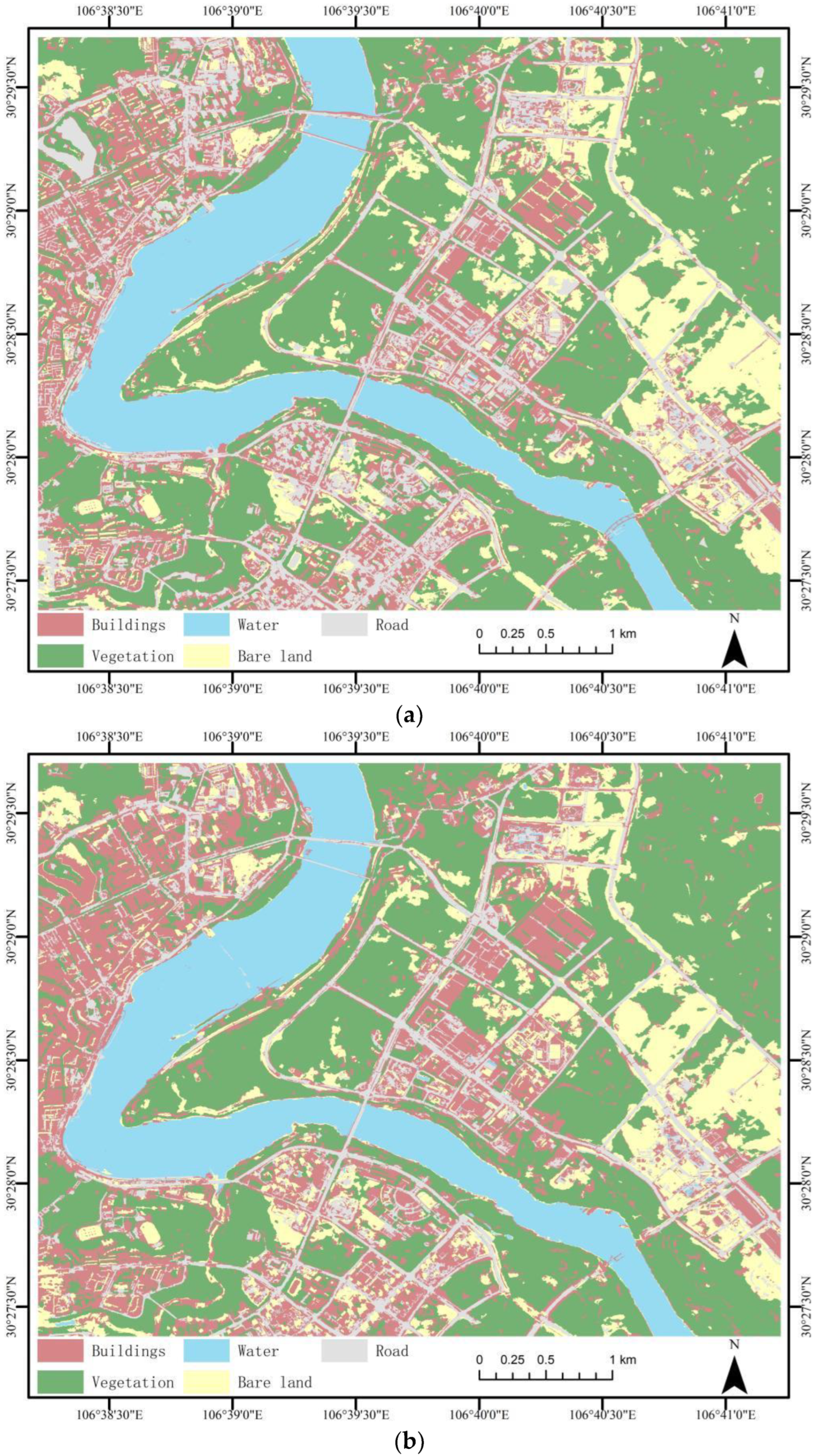
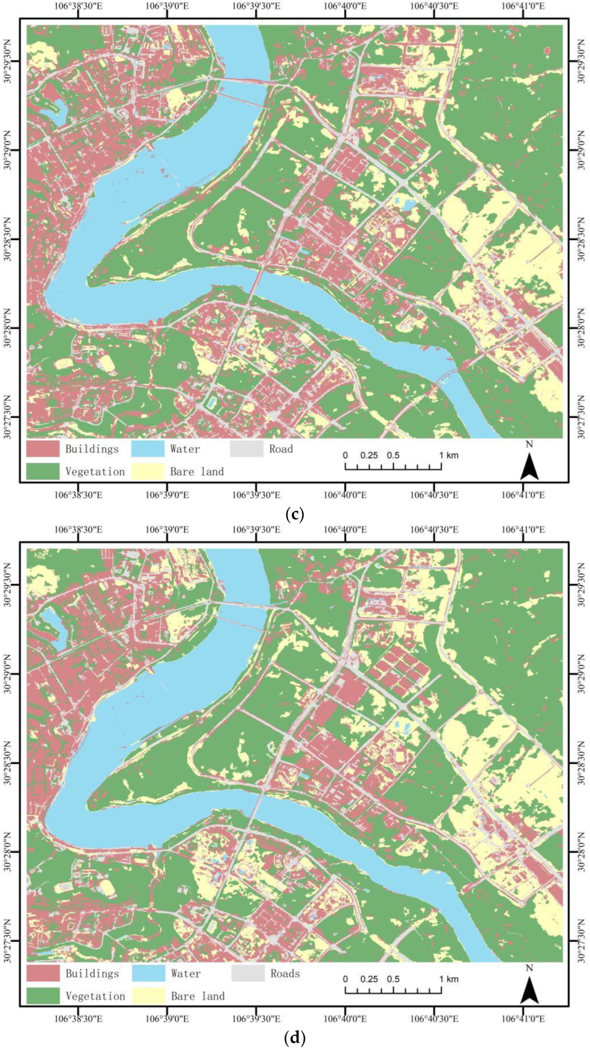
4.3. Classification Results

For further analysis, the optimal combinations of the four classification methods and five feature selection methods were selected—Fisher–CART, Fm–RF, Fm–kNN, and mRMR–SVM—and the classification graphs of these four combinations are shown in Figure 7. Meanwhile, in order to analyze the accuracy of the classified ground objects, the overall accuracy, as well as kappa coefficients, were calculated to evaluate the classification results, based on the decoded flags and visually decoded sample points, as shown in

Table 4. Accuracy of ground cover classification.

	Fisher-CART		Fm-RF		Fm-KNN		mRMR-SVM
	Producer’s accuracy	User’s accuracy	Producer’s accuracy	User’s accuracy	Producer’s accuracy	User’s accuracy	Producer’s accuracy	User’s accuracy
Roads	95.00%	76.61%	97.00%	93.26%	93.00%	95.87%	97.00%	89.81%
Buildings	74.00%	91.02%	85.00%	91.40%	92.00%	91.08%	85.00%	94.44%
Water	92.93%	97.87%	93.94%	97.90%	96.96%	98.96%	97.98%	98.97%
Bare land	97.14%	94.44%	100%	90.90%	98.57%	94.52%	98.57%	97.18%
Vegetation	99.33%	98.68%	99.33%	99.33%	99.33%	98.67%	99.33%	98.03%
Overall accuracy	91.52%		95.18%		96.14%		95.76%
Kappa	0.8923		0.939		0.951		0.9461

, as well as the specific land-cover classification accuracies.

From the analysis in Table 4, the producer’s and user’s accuracies for water, bare land, and vegetation in all four scenarios were greater than 94%. The water and vegetation extraction was improved, followed by that of bare land. The reason for this is that sparse grass can be classified as vegetation and bare land, and it is difficult to accurately determine which type the associated features belong to. The extraction effect of buildings and roads was relatively poor as the resolution of the images was high, and some narrow roads were interspersed among the buildings, making it easy to divide the roads and buildings together during segmentation, causing confusion between the two types of features. From the overall accuracy of the four schemes, the overall accuracy of Fm–RF, Fm–kNN, and mRMR–SVM were all greater than 95%, which indicates that Fm can better combine and optimize feature subsets and improve the classification ability of the used feature sets. All of the feature selection methods based on Fm could achieve effective surface feature information extraction. Meanwhile, the RFE and LR classification methods did not present high classification accuracy. Wrapper feature selection methods rely on feature models and specific machine learning algorithms, and the optimal feature combinations change as the learners change, which, in some cases, can have detrimental effects. In our experiment, there were negative values in the NDVI and NDWI feature values, and there was a data imbalance; for the embedded LR feature selection method, it is difficult to solve the data imbalance problem. In conclusion, both the single filtering feature selection methods and the combination of the proposed two filtering feature selection methods presented good performance, and filtering feature selection methods can more easily obtain better classification results when performing object-oriented classification.

4.4. Validation of the Fm Method

In order to test the effectiveness of the Fm method, we selected different research areas and GF-2 images and carried out experiments. The classification results and overall accuracy with different classifiers are shown in the Figure 8.

As shown in

Table 5. Overall accuracy and kappa coefficient of Fm with different classifiers.

	CART	RF	KNN	SVM
Overall accuracy	88.67%	92.04%	91.08%	88.68%
Kappa	0.8545	0.8979	0.8852	0.8546

, Fm achieves better classification results in the different study area. The overall accuracy of Fm with CART, RF, KNN, and SVM classifiers were 88.67%, 92.04%, 91.08%, and 88.68%, respectively. The kappa coefficient also reached 0.8545, 0.8979, 0.8852, and 0.8546, respectively. The overall accuracy of RF and KNN is better than that of the CART and SVM, which is consistent with the experimental results above. Verified experiments show that Fm can effectively reduce the dimensionality of high-dimensional data and obtain the optimal feature subset. RF and KNN classifiers are more suitable for image classification combined with Fm.

5. Conclusions

In this paper, an algorithm combining the Fisher Score and mRMR algorithms is proposed to address the problem of high dimensionality of the feature space in object-oriented classification. Although Fisher Score and mRMR feature selection methods have good applicability in feature screening, a single method cannot take into account the redundancy between features and the correlation between features and categories at the same time. The Fisher Score algorithm does not take into account the redundancy between features, and the mRMR algorithm cannot reflect the differences in the role of different features in classification. The combination of the Relief and mRMR algorithms can effectively make up for their shortcomings. After the experiments involving four different machine learning classification methods, the overall accuracy of Fm combined with RF and KNN is better than that of RF and CART.

Through a comparative test of four kinds of classifiers, we determined that: (1) Feature selection can allow for the elimination of redundant features, and high classification accuracy can still be achieved when using a small number of features. Accordingly, filtered feature selection methods were found to perform better than wrapped and embedded feature selection methods. (2) Two classifiers—RF and SVM—exhibited better stability than the other two classifiers as the number of features increased during the experiment. (3) In this study, the proposed Fm feature selection method was used in the classification experiment and showed the best performance when used with the RF and kNN classifiers, allowing for better optimization of the feature set. The final classification accuracy and efficiency were improved obviously by using the Fm feature subset. The overall accuracy of the Fm–RF and Fm–kNN approaches reached 95.18% and 96.14%, respectively. The kappa coefficient reached 0.939 and 0.951, respectively. Except for the mapping accuracy of Fm-RF construction land, the mapping accuracy and user accuracy of Fm-RF and Fm-KNN both reached more than 91%.

References

1. Muzirafuti, A.; Cascio, M.; Lanza, S.; Randazzo, G. UAV Photogrammetry-based Mapping of the Pocket Beaches of Isola Bella Bay, Taormina (Eastern Sicily). In Proceedings of the 2021 International Workshop on Metrology for the Sea; Learning to Measure Sea Health Parameters (MetroSea), Reggio Calabria, Italy, 4–6 October 2021; pp. 418–422. [Google Scholar]
2. Randazzo, G.; Italiano, F.; Micallef, A.; Tomasello, A.; Cassetti, F.P.; Zammit, A.; D’Amico, S.; Saliba, O.; Cascio, M.; Cavallaro, F.; et al. WebGIS Implementation for Dynamic Mapping and Visualization of Coastal Geospatial Data: A Case Study of BESS Project. Appl. Sci. 2021, 11, 8233. [Google Scholar] [CrossRef]
3. Hong, L.; Feng, Y.F.; Peng, H.Y.; Chu, S.S. Classification of high spatial resolution remote sensing imagery based on object-oriented multi-scale weighted sparse representation. Acta Geod. Cartogr. Sin. 2022, 51, 224–237. [Google Scholar] [CrossRef]
4. Wang, H.; Wang, C.B.; Wu, H.G. Using GF-2 Imagery and the Conditional Random Field Model for Urban Forest Cover Mapping. Remote Sens. Lett. 2016, 7, 378–387. [Google Scholar] [CrossRef]
5. Zhang, X.Y.; Feng, X.Z.; Jiang, H. Feature set optimization in object-oriented methodology. J. Remote Sens. 2009, 13, 664–669. [Google Scholar] [CrossRef]
6. Stefanos, G.; Tais, G.; Sabine, V.; Morutz, S.; Stamatis, K.; Eleonore, W. Less is more: Optimizing classification performance through feature selection in a very-high-resolution remote sensing object-based urban application. GISci. Remote Sens. 2018, 55, 221–242. [Google Scholar]
7. Xue, B.; Zhang, M.; Browne, W.N.; Yao, X. A Survey on Evolutionary Computation Approaches to Feature Selection. IEEE Trans. Evol. Comput. 2016, 20, 606–626. [Google Scholar] [CrossRef]
8. Li, J.; Cheng, K.; Wang, S.; Morstatter, F.; Trevino, R.P.; Tang, J.; Liu, H. Feature Selection: A Data Perspective. ACM Comput. Surv. (CSUR) 2017, 50, 1–45. [Google Scholar] [CrossRef]
9. Dokeroglu, T.; Deniz, A.; Kiziloz, H.E. A Comprehensive Survey on Recent Metaheuristics for Feature Selection. Neurocomputing 2022, 494, 269–296. [Google Scholar] [CrossRef]
10. Saúl, S.F.; Carrasco-Ochoa, J.A.; José, M.T. A new hybrid filter-wrapper feature selection method for clustering based on ranking. Neurocomputing 2016, 214, 866–880. [Google Scholar]
11. Zhao, L.; Gong, J.X.; Huang, D.R.; Hu, C. Fault feature selection method of gearbox based on Fisher Score and maximum information coefficient. Control. Decis. 2021, 36, 2234–2240. [Google Scholar] [CrossRef]
12. Zhou, Y.; Zhang, R.; Wang, S.X.; Wang, F.T. Feature Selection Method Based on High-Resolution Remote Sensing Images and the Effect of Sensitive Features on Classification Accuracy. Sensors 2018, 18, 2013. [Google Scholar] [CrossRef]
13. Liu, W.; Wang, J.Y. Recursive elimination–election algorithms for wrapper feature selection. Appl. Soft Comput. J. 2021, 113, 107956. [Google Scholar] [CrossRef]
14. Li, M.; Kamili, M. Research on Feature Selection Methods and Algorithms. Comput. Technol. Dev. 2013, 23, 16–21. [Google Scholar] [CrossRef]
15. Wu, D.; Guo, S.C. An improved Fisher Score feature selection method and its application. J. Liaoning Tech. Univ. (Nat. Sci.) 2019, 38, 472–479. [Google Scholar]
16. Gu, Q.Q.; Li, Z.H.; Han, J.W. Generalized Fisher Score for Feature Selection. arXiv 2012, arXiv:1202.3725. [Google Scholar]
17. Cheng, X.M.; Shen, Z.F.; Xing, T.Y.; Xia, L.G.; Wu, T.J. Efficiency and accuracy analysis of multi-spectral remote sensing image classification based on mRMR feature optimization algorithm. J. Geo-Inf. Sci. 2016, 18, 815–823. [Google Scholar] [CrossRef]
18. Chen, S.L.; Gao, X.X.; Liao, Y.F.; Deng, J.B.; Zhou, B. Wetland classification method of Dongting Lake district based on CART using GF-2 image. Bull. Surv. Map. 2021, 6, 12–15. [Google Scholar] [CrossRef]
19. Gómez, C.; Wulder, M.A.; Montes, F.; Delgado, J.A. Modeling Forest Structural Parameters in the Mediterranean Pines of Central Spain using QuickBird-2 Imagery and Classification and Regression Tree Analysis (CART). Remote Sens. 2012, 4, 135–159. [Google Scholar] [CrossRef]
20. Gu, H.Y.; Yan, L.; Li, H.T.; Jia, Y. An Object-based Automatic Interpretation Method for Geographic Features Based on Random Forest Machine Learning. Geomat. Inf. Sci. Wuhan Univ. 2016, 41, 228–234. [Google Scholar] [CrossRef]
21. Dennis, C.D.; Steven, E.F.; Monique, G.D. A comparison of pixel-based and object-based image analysis with selected machine learning algorithms for the classification of agricultural landscapes using SPOT-5 HRG imagery. Remote Sens. Environ. 2012, 118, 259–272. [Google Scholar]
22. Voisin, A.; Krylov, V.A.; Moser, G.; Serpico, S.B.; Zerubia, J. Supervised Classification of Multisensor and Multiresolution Remote Sensing Images with a Hierarchical Copula-Based Approach. IEEE Trans. Geosci. Remote Sens. 2014, 52, 3346–3358. [Google Scholar] [CrossRef]
23. Paradis, E. Probabilistic unsupervised classification for large-scale analysis of spectral imaging data. Int. J. Appl. Earth Obs. Geoinf. 2022, 107, 102675. [Google Scholar] [CrossRef]
24. Liu, S.; Jiang, Q.G.; Ma, Y.; Xiao, Y.; Li, Y.H.; Cui, C. Object-oriented Wetland Classification Based on Hybrid Feature Selection Method Combining with Relief F/Mult-objective Genetic. Trans. Chin. Soc. Agric. Mach. 2017, 48, 119–127. [Google Scholar] [CrossRef]
25. Zhang, W.Q.; Li, X.R.; Zhao, L.Y. Discovering the Representative Subset with Low Redundancy for Hyperspectral Feature Selection. Remote Sens. 2019, 11, 1341. [Google Scholar] [CrossRef]
26. Wang, L.; Gong, G.H. Multiple features remote sensing image classification based on combining ReliefF and mRMR. Chin. J. Stereol. Image 2014, 19, 250–257. [Google Scholar] [CrossRef]
27. Wu, Q.; Zhong, R.F.; Zhao, W.J.; Song, K.; Du, L.M. Land-cover classification using GF-2 images and airborne lidar data based on Random Forest. Int. J. Remote Sens. 2019, 40, 2410–2426. [Google Scholar] [CrossRef]
28. Shao, L.Y.; Zhou, Y. Application of improved oversampling algorithm in class-imbalance credit scoring. Appl. Res. Comput. 2019, 36, 1683–1687. [Google Scholar] [CrossRef]
29. Zhu, J.F.; Li, F.; Lu, B.X. Comparative Study of Fisher and KNN Discriminant Classification Algorithms Based on Clustering Improvement. J. Anhui Agric. Sci. 2019, 47, 250–252, 257. [Google Scholar]
30. Xu, X.Y.; Zhao, L.Z.; Chen, X.Y.; He, Z.C. Design of Convolutional Neural Network Based on Improved Fisher Discriminant Criterion. Comput. Eng. 2020, 46, 255–260, 266. [Google Scholar] [CrossRef]
31. Huang, L.S.; Ruan, C.; Huang, W.J.; Shi, Y.; Peng, D.L.; Ding, W.J. Wheat Powdery mildew monitoring based on GF-1 remote sensing image and relief-mRMR-GASVM model. Trans. Chin. Soc. Agric. Eng. 2018, 34, 167–175, 314. [Google Scholar] [CrossRef]
32. Özyurt, F. A fused CNN model for WBC detection with MRMR feature selection and extreme learning machine. Soft Comput. 2020, 24, 163–8172. [Google Scholar] [CrossRef]
33. Huang, L.; Xiang, Z.J.; Chu, H. Remote sensing image classification algorithm based on mRMR selection and IFCM clustering. Bull. Surv. Map. 2019, 4, 32–37. [Google Scholar] [CrossRef]
34. Zhang, X.L.; Zhang, F.; Zhou, N.; Zhang, J.J.; Liu, W.F.; Zhang, S.; Yang, X.J. Near-Infrared Spectral Feature Selection of Water-Bearing Rocks Based on Mutual Information. Spectrosc. Spectr. Anal. 2021, 41, 2028–2035. [Google Scholar] [CrossRef]
35. Wu, C.W.; Liang, J.H.; Wang, W.; Li, C.S. Random Forest Algorithm Based on Recursive Feature Elimination. Stat. Decis. 2017, 21, 60–63. [Google Scholar] [CrossRef]
36. Fan, T.C.; Jia, Y.F.; Li, Y.F.; Zhao, J.L. Prediction of Gully Distribution Probability in Yanhe Basin Based on Remote Sensing lmage and Logistic Regression Model. Res. Soil Water Conserv. 2022, 29, 316–321. [Google Scholar] [CrossRef]
37. Luo, H.X.; Li, M.F.; Dai, S.P.; Li, H.L.; Li, Y.P.; Hu, Y.Y.; Zheng, Q.; Yu, X.; Fang, J.H. Combinations of Feature Selection and Machine Learning Algorithms for Object-Oriented Betel Palms and Mango Plantations Classification Based on Gaofen-2 Imagery. Remote Sens. 2022, 14, 1757. [Google Scholar] [CrossRef]
38. Lu, L.Z.; Tao, Y.; Di, L.P. Object-Based Plastic-Mulched Landcover Extraction Using Integrated Sentinel-1 and Sentinel-2 Data. Remote Sens. 2018, 10, 1820. [Google Scholar] [CrossRef]
39. Yang, H.B.; Li, F.; Wang, W.; Yu, K. Estimating Above-Ground Biomass of Potato Using Random Forest and Optimized Hyperspectral Indices. Remote Sens. 2021, 13, 2339. [Google Scholar] [CrossRef]
40. Wang, G.Z.; Jin, H.L.; Gu, X.H.; Yang, G.J.; Feng, H.K.; Sun, Q. Remote Sensing Classification of Autumn Crops Based on Hybrid Feature Selection Model Combining with Relief F and Improved Separability and Thresholds. Trans. Chin. Soc. Agric. Mach. 2021, 52, 199–210. [Google Scholar] [CrossRef]
41. Garg, R.; Kumar, A.; Prateek, M.; Pandey, K.; Kumar, S. Land Cover Classification of Spaceborne Multifrequency SAR and Optical Multispectral Data using Machine Learning. Adv. Space Res. 2021, 69, 1726–1742. [Google Scholar] [CrossRef]
42. Zhang, S.; Huang, H.; Huang, Y.; Cheng, D.; Huang, J. A GA and SVM Classification Model for Pine Wilt Disease Detection Using UAV-Based Hyperspectral Imagery. Appl. Sci. 2022, 12, 6676. [Google Scholar] [CrossRef]
43. Hu, J.M.; Dong, Z.Y.; Yang, X.Z. Object-oriented High-resolution Remote Sensing Image lnformation Extraction Method. Geospat. Inf. 2021, 19, 10–13, 18, 157. [Google Scholar] [CrossRef]
44. Hao, S.; Cui, Y.; Wang, J. Segmentation Scale Effect Analysis in the Object-Oriented Method of High-Spatial-Resolution Image Classification. Sensors 2021, 21, 7935. [Google Scholar] [CrossRef] [PubMed]
Figure 1. Location and imaging of the study area: (a) administrative boundary map of Sichuan Province; (b) pre-processed image.
Applsci 12 08845 g001
Figure 2. Technical flow chart.
Applsci 12 08845 g002
Figure 3. Typical ground object segmentation plot: (a) buildings; (b) water; (c) roads; (d) bare land.
Applsci 12 08845 g003aApplsci 12 08845 g003b
Figure 4. The correlation matrix of the top 15 features of the five feature selection methods: (a) Fm; (b) Fisher; (c) mRMR; (d) RFE; (e) LR.
Applsci 12 08845 g004aApplsci 12 08845 g004b
Figure 5. The variation trend of number of features and overall accuracy of five feature selection methods with different classifiers: (a) CART; (b) RF; (c) KNN; (d) SVM.
Applsci 12 08845 g005aApplsci 12 08845 g005b
Figure 6. The optimal accuracy of four features with different classifiers was selected.
Applsci 12 08845 g006
Figure 7. Graph of optimal classification results for different classifiers (a) Fisher-CART; (b) Fm-RF; (c) Fm-KNN; (d) mRMR-SVM.
Applsci 12 08845 g007aApplsci 12 08845 g007b
Figure 8. Fm classification image with different classifiers: (a) CART; (b) RF; (c) KNN; (d) SVM.
Applsci 12 08845 g008aApplsci 12 08845 g008b