Enhancement of In-Plane Seismic Full Waveform Inversion with CPU and GPU Parallelization

 ,
,  ,
,  , , and
Abstract
1. Introduction
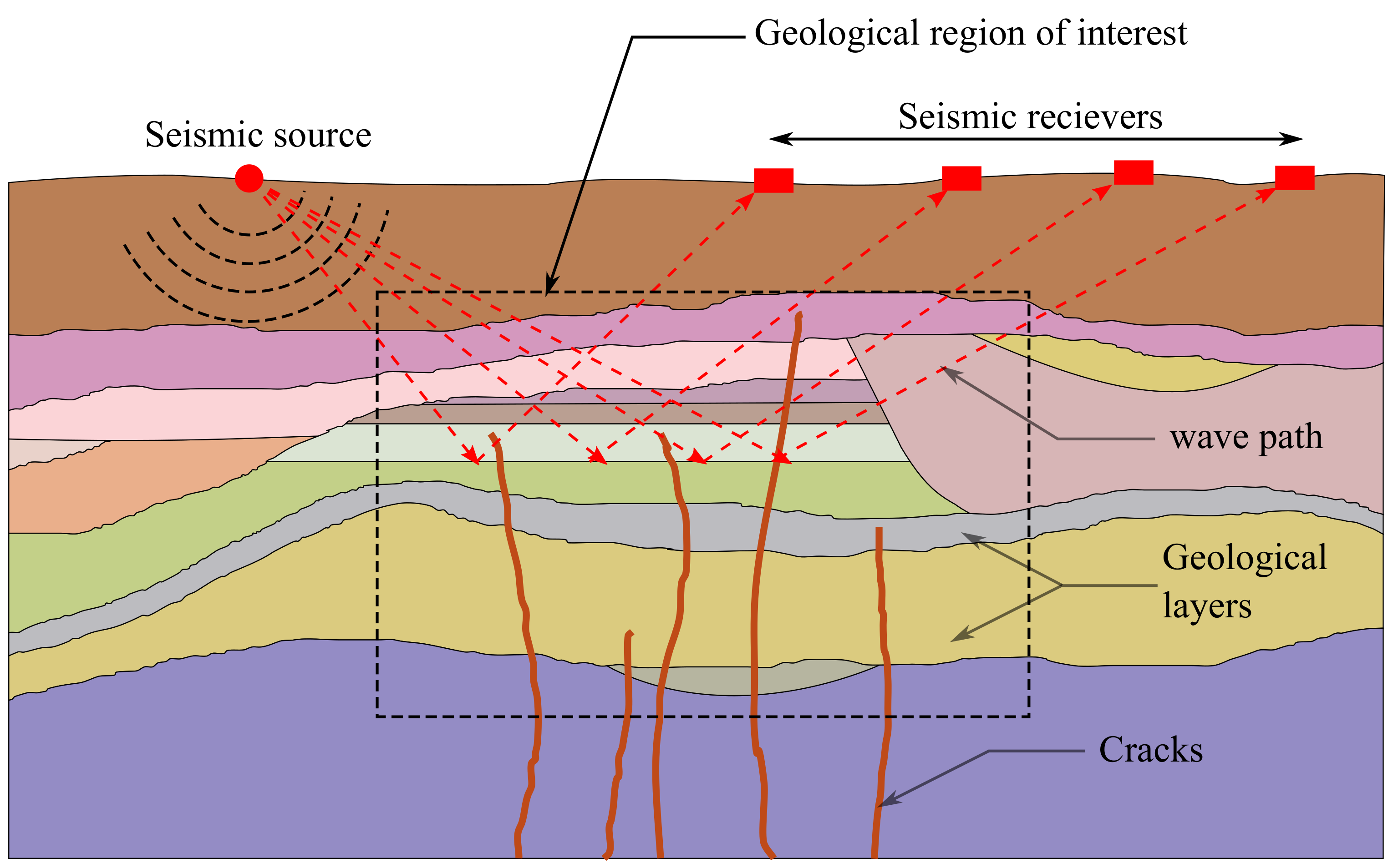
1.1. The Seismic Full Waveform Inversion
1.2. Parallel Computation
1.3. Importance, Scope and Limitations of the Study
2. Mathematical Model
2.1. Stress Velocity Formulation of 2D Elastic Wave Equation
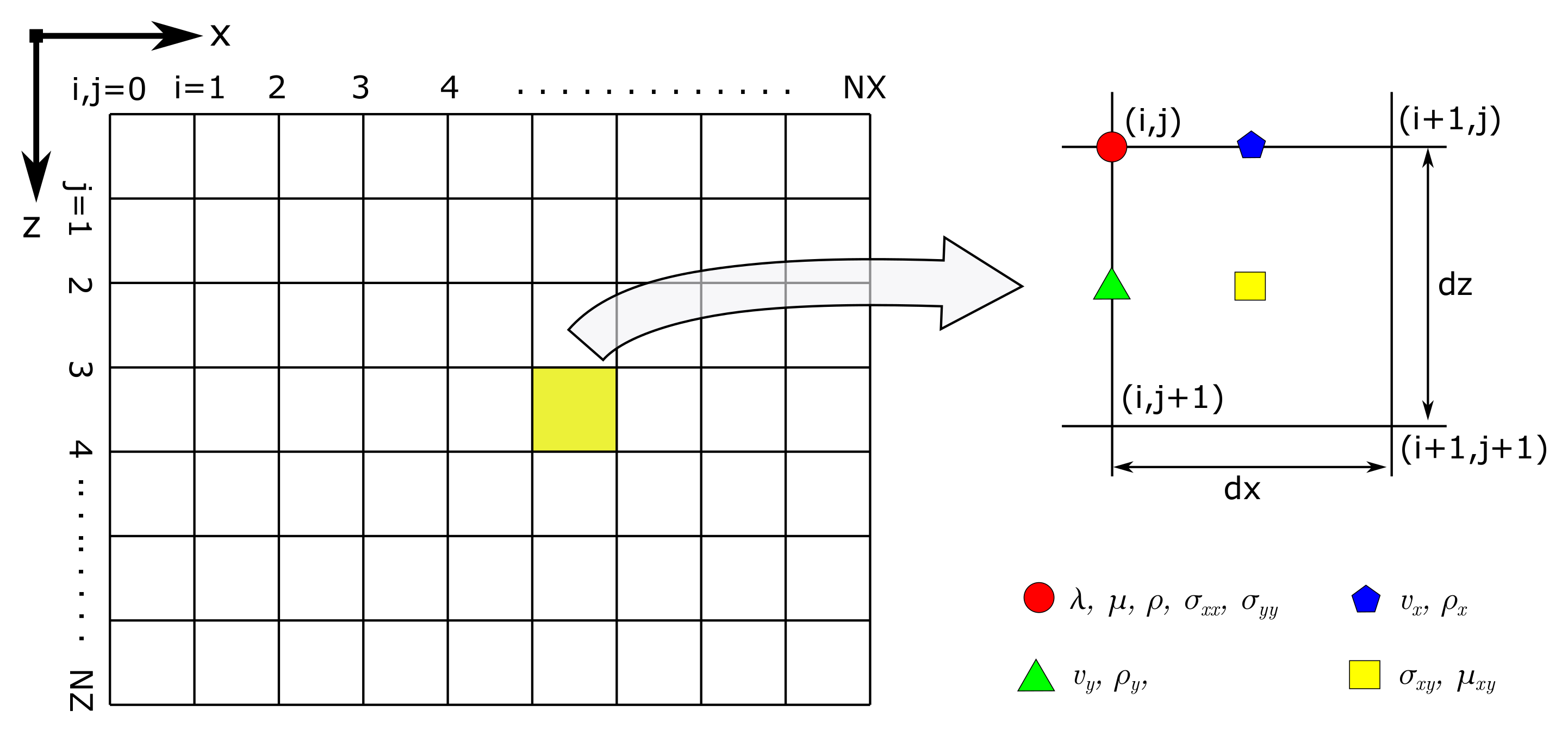
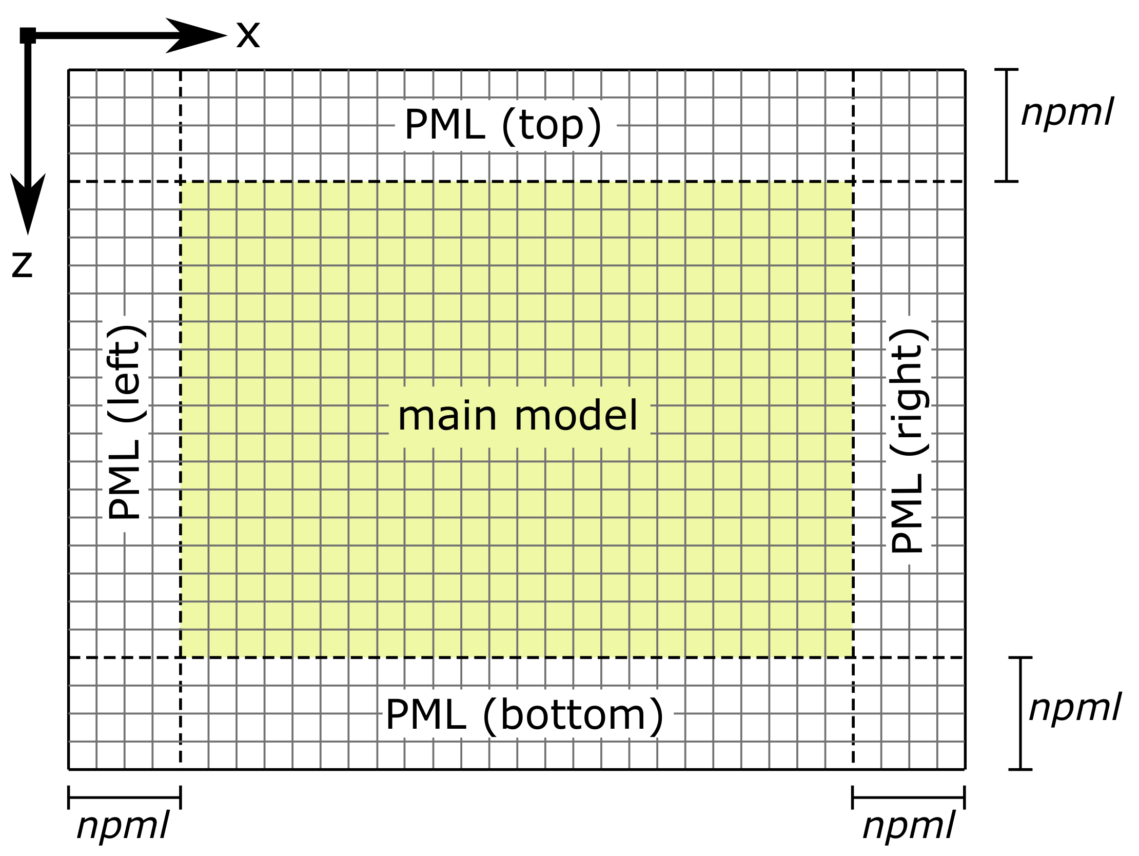
2.2. Numerical Implementation in FDM
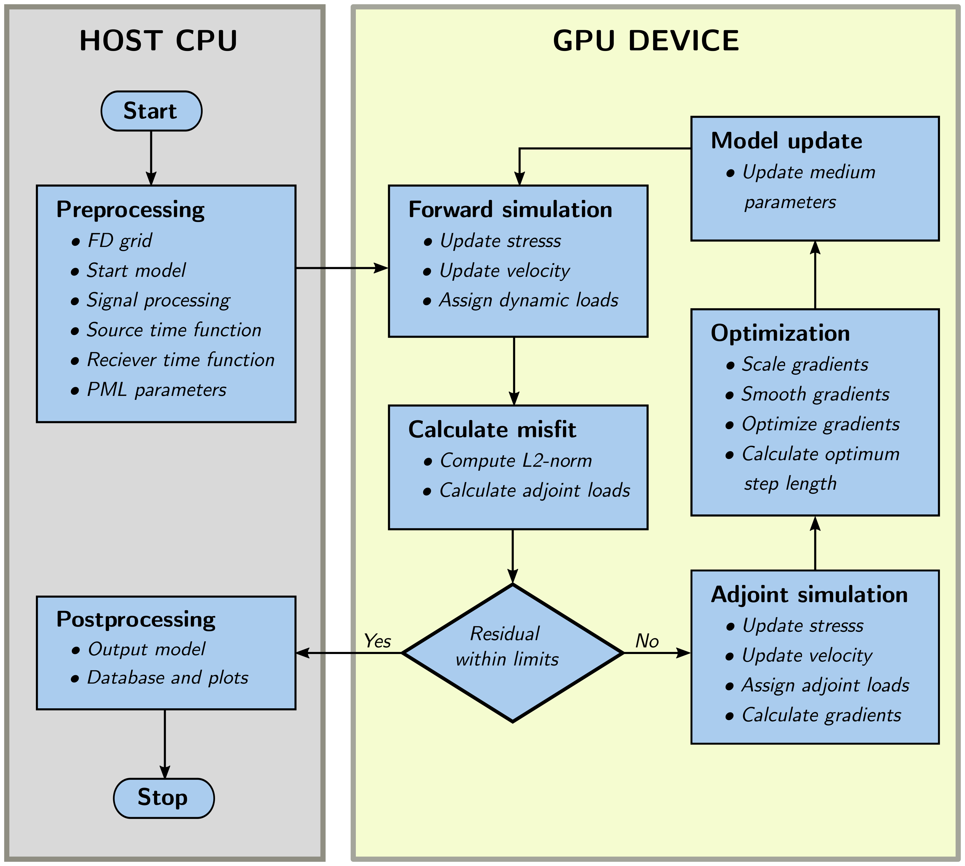
3. Parallel Computational Model
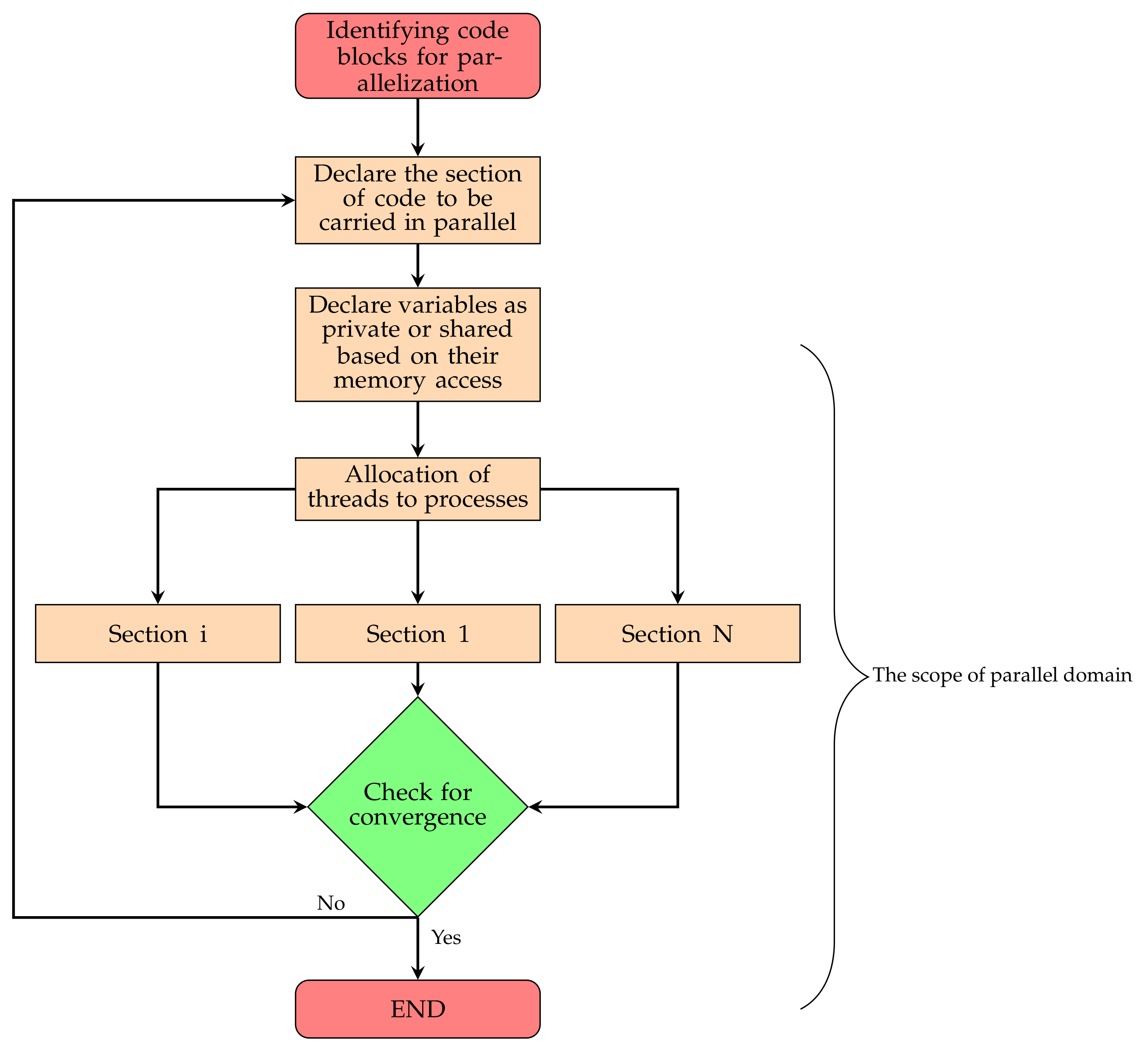
3.1. OpenMP
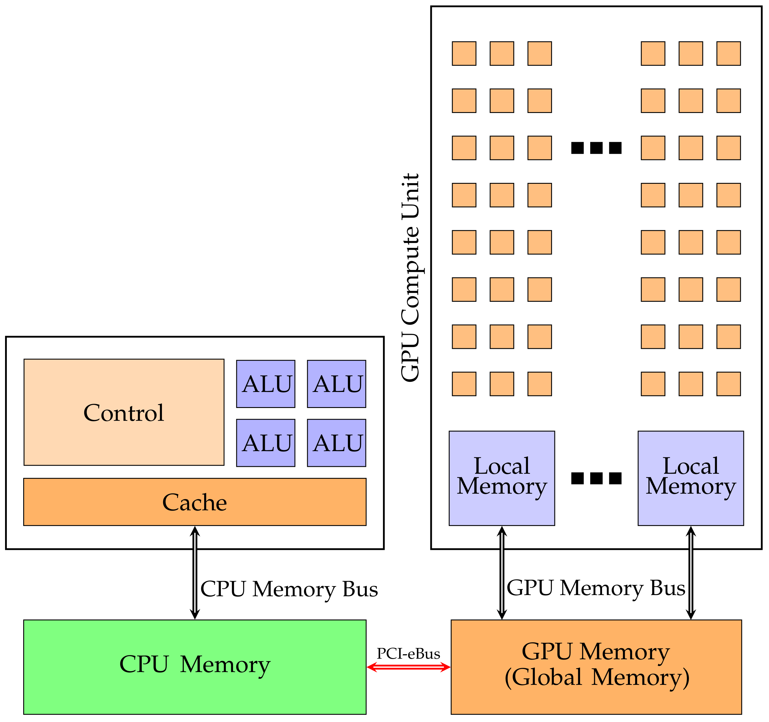
3.2. GPU
Compute Unified Device Architecture (CUDA)
4. Numerical Simulations
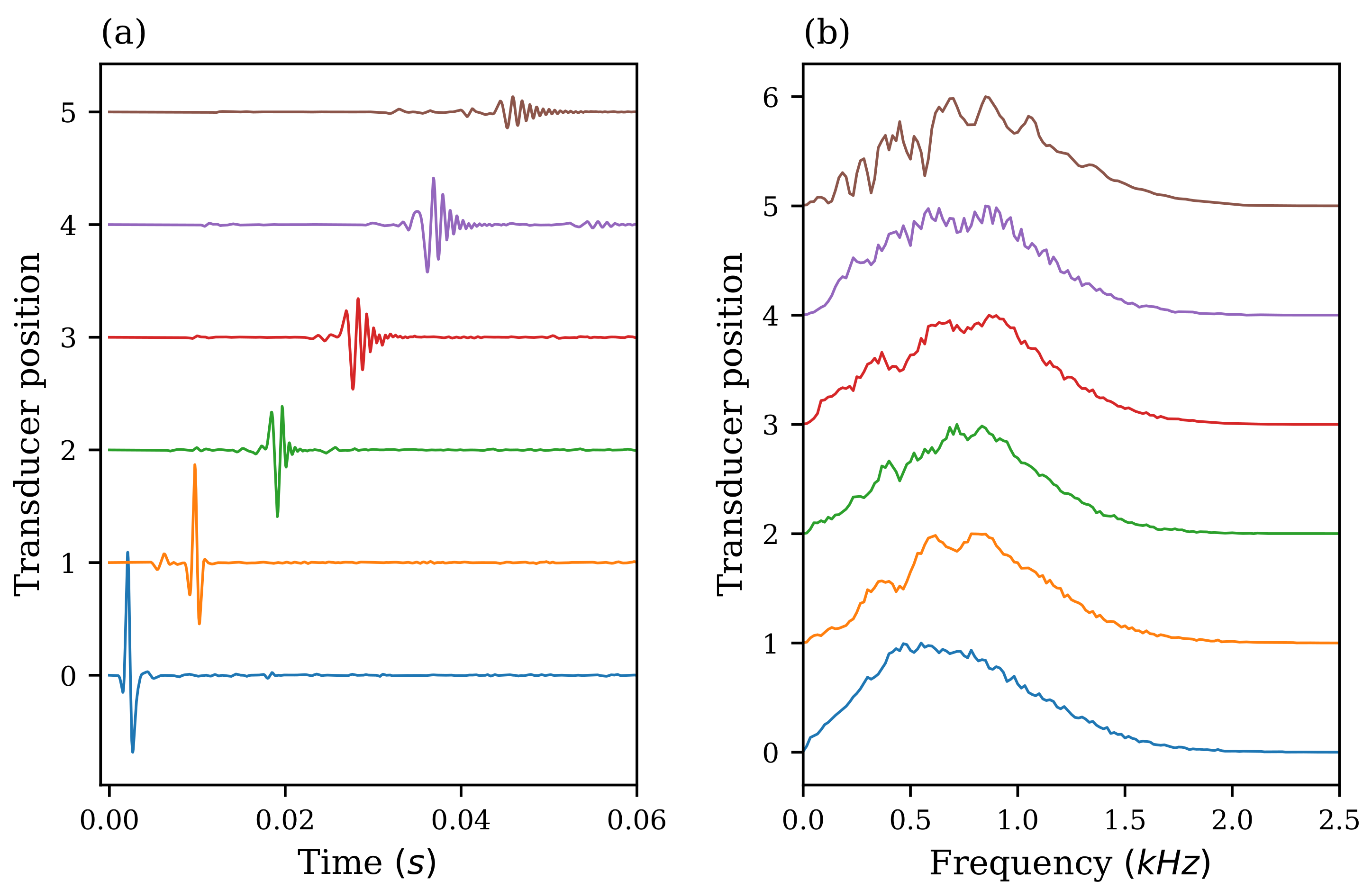
4.1. Seismic Forward Model
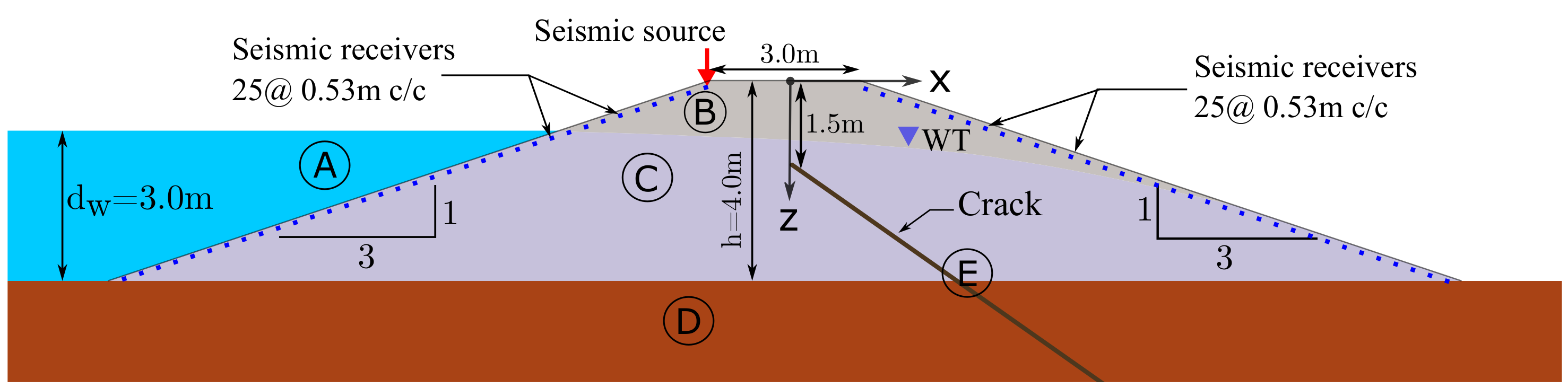
4.2. Seismic FWI Model
5. Results and Discussion
6. Conclusions
Author Contributions
Funding
Institutional Review Board Statement
Informed Consent Statement
Data Availability Statement
Acknowledgments
Conflicts of Interest
References
- Guasch, L.; Calderón Agudo, O.; Tang, M.X.; Nachev, P.; Warner, M. Full-waveform inversion imaging of the human brain. NPJ Digit. Med. 2019, 3, 1–12. [Google Scholar] [CrossRef]
- Gauthier, O.; Virieux, J.; Tarantola, A. Two-dimensional nonlinear inversion of seismic waveforms: Numerical results. Geophysics 1986, 51, 1387–1403. [Google Scholar] [CrossRef]
- Gauthier, O.; Virieux, J.; Tarantola, A. Nonlinear inversion of seismic reflection data. In SEG Technical Program Expanded Abstracts 1985; Society of Exploration Geophysicists: Houston, TX, USA, 2005; pp. 390–393. [Google Scholar] [CrossRef]
- Mora, P. Nonlinear two-dimensional elastic inversion of multi offset seismic data. Geophysics 1987, 52, 1211–1228. [Google Scholar] [CrossRef]
- Tarantola, A. Inversion of seismic reflection data in the acoustic approximation. Geophysics 1984, 49, 1259–1266. [Google Scholar] [CrossRef]
- Tarantola, A. Linearized inversion of seismic reflection data. Geophys. Prospect. 1984, 32, 998–1015. [Google Scholar] [CrossRef]
- Tarantola, A. Theoretical background for the inversion of seismic waveforms including elasticity and attenuation. Pure Appl. Geophys. 1988, 128, 365–399. [Google Scholar] [CrossRef]
- Pratt, R.G.; Worthington, M.H. Inverse Theory Applied To Multi-Source Cross-Hole Tomography. Geophys. Prospect. 1990, 38, 287–310. [Google Scholar] [CrossRef]
- Pratt, R.G. Inverse Theory Applied To Multi-Source Cross-Hole Tomography. Geophys. Prospect. 1990, 38, 311–329. [Google Scholar] [CrossRef]
- Sourbier, F.; Operto, S.; Virieux, J.; Amestoy, P.; L’Excellent, J.Y. FWT2D: A massively parallel program for frequency-domain full-waveform tomography of wide-aperture seismic data-Part 2: Numerical examples and scalability analysis. Comput. Geosci. 2009, 35, 496–514. [Google Scholar] [CrossRef]
- Sourbier, F.; Operto, S.; Virieux, J.; Amestoy, P.; L’Excellent, J.Y. FWT2D: A massively parallel program for frequency-domain full-waveform tomography of wide-aperture seismic data-Part 1: Algorithm. Comput. Geosci. 2009, 35, 487–495. [Google Scholar] [CrossRef]
- Köhn, D. Time Domain 2D Elastic Full Waveform Tomography. Ph.D. Thesis, Kiel University, Kiel, Germany, 2011. [Google Scholar]
- Yang, P.; Brossier, R.; Métivier, L.; Virieux, J.; Zhou, W. A Time-Domain Preconditioned Truncated Newton Approach to Visco-acoustic Multiparameter Full Waveform Inversion. SIAM J. Sci. Comput. 2018, 40, B1101–B1130. [Google Scholar] [CrossRef]
- Wei, Z.F.; Gao, H.W.; Zhang, J.F. Time-domain full waveform inversion based on an irregular-grid acoustic modeling method. Chin. J. Geophys. 2014, 57, 586–594. (In Chinese) [Google Scholar] [CrossRef]
- Charara, M.; Barnes, C.; Tarantola, A. Full waveform inversion of seismic data for a viscoelastic medium. Methods Appl. Invers. 2000, 92, 68–81. [Google Scholar] [CrossRef]
- Fabien-Ouellet, G.; Gloaguen, E.; Giroux, B. Time domain viscoelastic full waveform inversion. Geophys. J. Int. 2017, 209, 1718–1734. [Google Scholar] [CrossRef]
- Pan, W.; Innanen, K.A.; Wang, Y. SeisElastic2D: An open-source package for multiparameter full-waveform inversion in isotropic-, anisotropic- and visco-elastic media. Comput. Geosci. 2020, 145, 104586. [Google Scholar] [CrossRef]
- Chen, J.B.; Cao, J. Modeling of frequency-domain elastic-wave equation with an average-derivative optimal method. Geophysics 2016, 81, T339–T356. [Google Scholar] [CrossRef][Green Version]
- Moczo, P. Introduction to Modeling Seismic Wave Propagation by the Finite-Difference Methods. In Disaster Prevention Research Institute; Kyoto University: Kyoto, Japan, 1998. [Google Scholar]
- Moczo, P.; Robertsson, J.O.A.; Eisner, L. The finite-difference time-domain method for modeling of seismic wave propagation. Adv. Geophys. 2007, 48, 421–516. [Google Scholar]
- Abubakar, A.; Pan, G.; Li, M.; Zhang, L.; Habashy, T.; van den Berg, P. Three-dimensional seismic full-waveform inversion using the finite-difference contrast source inversion method. Geophys. Prospect. 2011, 59, 874–888. [Google Scholar] [CrossRef]
- Fang, J.; Chen, H.; Zhou, H.; Rao, Y.; Sun, P.; Zhang, J. Elastic Full-Waveform Inversion Based on GPU Accelerated Temporal Fourth-Order Finite-Difference Approximation. Comput. Geosci. 2020, 135. [Google Scholar] [CrossRef]
- Wang, K.; Guo, M.; Xiao, Q.; Ma, C.; Zhang, L.; Xu, X.; Li, M.; Li, N. Frequency Domain Full Waveform Inversion Method of Acquiring Rock Wave Velocity in Front of Tunnels. Appl. Sci. 2021, 11, 6330. [Google Scholar] [CrossRef]
- Komatitsch, D.; Martin, R. An unsplit convolutional perfectly matched layer improved at grazing incidence for the seismic wave equation. Geophysics 2007, 72, SM155–SM167. [Google Scholar] [CrossRef]
- Martin, R.; Komatitsch, D.; Ezziani, A. An unsplit convolutional perfectly matched layer improved at grazing incidence for seismic wave propagation in poroelastic media. Geophysics 2008, 73, T51–T61. [Google Scholar] [CrossRef]
- Martin, R.; Komatitsch, D. An unsplit convolutional perfectly matched layer technique improved at grazing incidence for the viscoelastic wave equation. Geophys. J. Int. 2009, 179, 333–344. [Google Scholar] [CrossRef]
- Li, L.; Tan, J.; Schwarz, B.; Staněk, F.; Poiata, N.; Shi, P.; Diekmann, L.; Eisner, L.; Gajewski, D. Recent Advances and Challenges of Waveform-Based Seismic Location Methods at Multiple Scales. Rev. Geophys. 2020, 58, e2019RG000667. [Google Scholar] [CrossRef]
- Jiang, J.; Zhu, P. Acceleration for 2D time-domain elastic full waveform inversion using a single GPU card. J. Appl. Geophys. 2018, 152, 173–187. [Google Scholar] [CrossRef]
- Wang, B.; Gao, J.; Zhang, H.; Zhao, W. CUDA-based acceleration of full waveform inversion on GPU. In SEG Technical Program Expanded Abstracts 2011; SEG: Houston, TX, USA, 2012; pp. 2528–2533. [Google Scholar] [CrossRef]
- Michéa, D.; Komatitsch, D. Accelerating a three-dimensional finite-difference wave propagation code using GPU graphics cards. Geophys. J. Int. 2010, 182, 389–402. [Google Scholar] [CrossRef]
- Köhn, D.; Kurzmann, A. DENISE User Manual; Kiel University: Kiel, Germany, 2014. [Google Scholar]
- Levander, A. Fourth-order finite-difference P-S. Geophysics 1988, 53, 1425–1436. [Google Scholar] [CrossRef]
- Virieux, J. P-SV wave propagation in heterogeneous media: Velocity-stress finite-difference method. Geophysics 1986, 51, 889–901. [Google Scholar] [CrossRef]
- Ross, P.E. Why CPU Frequency Stalled. IEEE Spectrum 2008, 45, 72. [Google Scholar] [CrossRef]
- Ramanathan, R. White Paper Intel® Multi-Core Processors: Making the Move to Quad-Core and Beyond. In White Paper From Intel 424 Corporation; Intel: Santa Clara, CA, USA, 2006. [Google Scholar]
- Robey, R.; Zamora, Y. Parallel and High Performance Computing; Simon and Schuster: New York, NY, USA, 2021. [Google Scholar]
- Memeti, S.; Li, L.; Pllana, S.; Kołodziej, J.; Kessler, C. Benchmarking OpenCL, OpenACC, OpenMP, and CUDA: Programming productivity, performance, and energy consumption. In Proceedings of the 2017 Workshop on Adaptive Resource Management and Scheduling for Cloud Computing, Washington, DC, USA, 28 July 2017; pp. 1–6. [Google Scholar]
- Chandra, R.; Dagum, L.; Kohr, D.; Maydan, D.; McDonald, J.; Menon, R. Parallel Programming in OpenMP; Morgan Kaufmann Publishers Inc.: San Francisco, CA, USA, 2001. [Google Scholar]
- Gimenes, T.L.; Pisani, F.; Borin, E. Evaluating the Performance and Cost of Accelerating Seismic Processing with CUDA, OpenCL, OpenACC, and OpenMP. In Proceedings of the 2018 IEEE International Parallel and Distributed Processing Symposium, IPDPS 2018, Vancouver, BC, Canada, 21–25 May 2018; pp. 399–408. [Google Scholar] [CrossRef]
- Santamarina, J.C.; Rinaldi, V.A.; Fratta, D.; Klein, K.; Wang, Y.H.; Cho, G.C.; Cascante, G. A Survey of Elastic and Electromagnetic Properties of Near-Surface Soils; SEG: Houston, TX, USA, 2009. [Google Scholar]
- Rizvi, Z.H.; Akhtar, S.J.; Haider, H.; Follmann, J.; Wuttke, F. Estimation of seismic wave velocities of metamorphic rocks using artificial neural network. Mater. Today Proc. 2020, 26, 324–330. [Google Scholar] [CrossRef]
- Wuttke, F.; Lyu, H.; Sattari, A.S.; Rizvi, Z.H. Wave based damage detection in solid structures using spatially asymmetric encoder–decoder network. Sci. Rep. 2021, 11, 20968. [Google Scholar] [CrossRef] [PubMed]


| OpenMP | CUDA | |
|---|---|---|
| Parallelism | -Data Parallelism | -Data Parallelism |
| -Asynchronous task parallelism | -Asynchronous task parallelism | |
| -Host and device | -Device only | |
| Architecture abstraction | -Memory hierarchy | -Memory hierarchy |
| -Data and computation binding | -Explicit data mapping and movement | |
| -Explicit data mapping and movement | ||
| Synchronisation | -Barrier | -Barrier |
| -Reduction | ||
| -Joint | ||
| Framework Implementation | -Compiler directives for C/C++ and Fortran | C/C++ extensions |
| Hardware | CPU/GPU | Memory | OS |
|---|---|---|---|
| CPU1 | 11th Gen Intel(R) Core(TM) i5-1135G7 @ 2.40 GHz | 8 GB | Ubuntu 20.04 |
| CPU2 | AMD Ryzen Threadripper 3970X(2.9 GHz) | 64 GB | Ubuntu 20.04 |
| GPU1 | Nvidia GeForce GTX 1650 | 4 GB | Ubuntu 20.04 |
| GPU2 (installed with CPU2) | Nvidia GeForce GTX 2080 Ti | 8 GB | Ubuntu 20.04 |
| Medium | Code | P-Wave Velocity | S-Wave Velocity ) | Density |
|---|---|---|---|---|
| Water | A | 1482 m/s | 1000 kg/m | |
| Unsaturated soil in the dam | B | 800 m/s | 400 m/s | 1700 kg/m |
| Saturated soil in the dam | C | 1450 m/s | 400 m/s | 1950 kg/m |
| Subsurface layers | D | 1900 m/s | 700 m/s | 2100 kg/m |
| Crack filler | E | 1600 m/s | 100 m/s | 1000 kg/m |
Publisher’s Note: MDPI stays neutral with regard to jurisdictional claims in published maps and institutional affiliations. |
© 2022 by the authors. Licensee MDPI, Basel, Switzerland. This article is an open access article distributed under the terms and conditions of the Creative Commons Attribution (CC BY) license (https://creativecommons.org/licenses/by/4.0/).
Share and Cite
Basnet, M.B.; Anas, M.; Rizvi, Z.H.; Ali, A.H.; Zain, M.; Cascante, G.; Wuttke, F. Enhancement of In-Plane Seismic Full Waveform Inversion with CPU and GPU Parallelization. Appl. Sci. 2022, 12, 8844. https://doi.org/10.3390/app12178844
Basnet MB, Anas M, Rizvi ZH, Ali AH, Zain M, Cascante G, Wuttke F. Enhancement of In-Plane Seismic Full Waveform Inversion with CPU and GPU Parallelization. Applied Sciences. 2022; 12(17):8844. https://doi.org/10.3390/app12178844
Chicago/Turabian StyleBasnet, Min Bahadur, Mohammad Anas, Zarghaam Haider Rizvi, Asmer Hamid Ali, Mohammad Zain, Giovanni Cascante, and Frank Wuttke. 2022. "Enhancement of In-Plane Seismic Full Waveform Inversion with CPU and GPU Parallelization" Applied Sciences 12, no. 17: 8844. https://doi.org/10.3390/app12178844
APA StyleBasnet, M. B., Anas, M., Rizvi, Z. H., Ali, A. H., Zain, M., Cascante, G., & Wuttke, F. (2022). Enhancement of In-Plane Seismic Full Waveform Inversion with CPU and GPU Parallelization. Applied Sciences, 12(17), 8844. https://doi.org/10.3390/app12178844