
A Review of Ensemble Learning Algorithms Used in Remote Sensing Applications


Abstract
:1. Introduction
2. Principles of Ensemble Learning Algorithms
2.1. Bagging Algorithms
2.2. Boosting Algorithms
2.3. Stacked Generalization
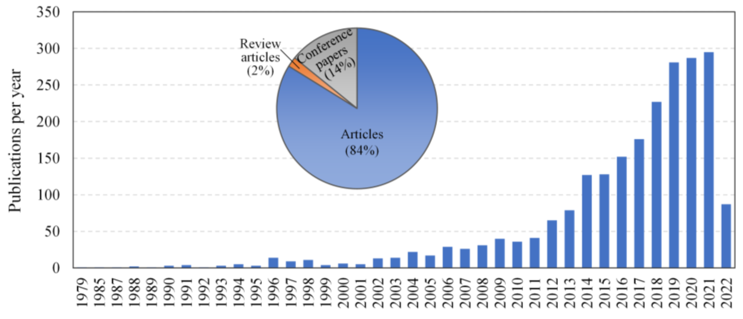
3. Literature Search and Analysis
4. Applications of Ensemble Learning Algorithms
4.1. Yield Prediction
4.2. Estimation of Forest Structure Parameters and Biomass
4.3. Natural Hazards
4.4. Spatial Downscaling
4.5. Other Applications
5. Discussion and Future Directions
5.1. Combining Feature Selection with Ensemble Learning
5.2. Other Ensemble Learning Algorithms
5.3. Deep Learning Algorithms
6. Conclusions
Funding
Conflicts of Interest
Nomenclature
| AdaBoost | adaptive boosting |
| ANN | artificial neural networks |
| ARMA | autoregressive–moving-average |
| ARIMA | autoregressive integrated moving average |
| BPNN | back propagation neural network |
| BRT | boosted regression tree |
| CART | classification and regression trees |
| CatBoost | categorical boosting |
| CNN | convolutional neural networks |
| DBN | deep belief network |
| DL | deep learning |
| DT | decision tree |
| EBF | evidence belief function |
| ELM | extreme learning machine |
| ENR | elastic net regression |
| ERT | extremely randomized trees |
| FDA | flexible discriminant analysis |
| GBDT | gradient boosting decision tree |
| GBRT | gradient boosting regression tree |
| GLM | generalized logistic models |
| GP | Gaussian process |
| kNN | k-nearest neighbor |
| LMT | logistic model tree |
| LR | linear regression |
| LSSVM | least square support vector machine |
| LWLR | locally weighted linear regression |
| MADT | multiclass alternating decision trees |
| MARS | multivariate adaptive regression splines |
| MLP | multilayer perceptron |
| MLR | multiple linear regression |
| PRF | parallel random forest |
| REPT | reduced error pruning tree |
| ResNet | residual neural network |
| RF | random forest |
| RR | ridge regression |
| RRF | regularized random forest |
| RT | regression tree |
| SGB | stochastic gradient boosting |
| SVM | support vector machine |
| SVR | support vector regression |
| VFI | voting feature interval |
| XGBoost | extreme gradient boosting |
References
- Navalgund, R.R.; Jayaraman, V.; Roy, P.S. Remote sensing applications: An overview. Curr. Sci. 2007, 93, 1747–1766. [Google Scholar]
- Weiss, M.; Jacob, F.; Duveiller, G. Remote sensing for agricultural applications: A meta-review. Remote Sens. Environ. 2020, 236, 111402. [Google Scholar] [CrossRef]
- Roy, P.S.; Behera, M.D.; Srivastav, S.K. Satellite Remote Sensing: Sensors, Applications and Techniques. Proc. Natl. Acad. Sci. India Sect. A Phys. Sci. 2017, 87, 465–472. [Google Scholar] [CrossRef]
- Myneni, R.B.; Maggion, S.; Iaquinta, J.; Privette, J.L.; Gobron, N.; Pinty, B.; Kimes, D.S.; Verstraete, M.M.; Williams, D.L. Optical remote sensing of vegetation: Modeling, caveats, and algorithms. Remote Sens. Environ. 1995, 51, 169–188. [Google Scholar] [CrossRef]
- Bonan, G.B.; Levis, S.; Sitch, S.; Vertenstein, M.; Oleson, K.W. A dynamic global vegetation model for use with climate models: Concepts and description of simulated vegetation dynamics. Glob. Change Biol. 2003, 9, 1543–1566. [Google Scholar] [CrossRef]
- Jacquemoud, S.; Verhoef, W.; Baret, F.; Bacour, C.; Zarco-Tejada, P.J.; Asner, G.P.; François, C.; Ustin, S.L. PROSPECT+SAIL models: A review of use for vegetation characterization. Remote Sens. Environ. 2009, 113, S56–S66. [Google Scholar] [CrossRef]
- Pan, M.; Sahoo, A.K.; Wood, E.F. Improving soil moisture retrievals from a physically-based radiative transfer model. Remote Sens. Environ. 2014, 140, 130–140. [Google Scholar] [CrossRef]
- Schulze, E.-D.; Beck, E.; Buchmann, N.; Clemens, S.; Müller-Hohenstein, K.; Scherer-Lorenzen, M. Dynamic Global Vegetation Models. In Plant Ecology; Springer: Berlin, Heidelberg, Germany, 2019; pp. 843–863. [Google Scholar]
- García-Haro, F.J.; Gilabert, M.A.; Meliá, J. A radiosity model for heterogeneous canopies in remote sensing. J. Geophys. Res. Atmos. 1999, 104, 12159–12175. [Google Scholar] [CrossRef]
- Lary, D.; Remer, L.; MacNeill, D.; Roscoe, B.; Paradise, S. Machine learning and bias correction of MODIS aerosol optical depth. IEEE Geosci. Remote Sens. Lett. 2009, 6, 694–698. [Google Scholar] [CrossRef]
- Ma, L.; Liu, Y.; Zhang, X.; Ye, Y.; Yin, G.; Johnson, B.A. Deep learning in remote sensing applications: A meta-analysis and review. ISPRS J. Photogramm. Remote Sens. 2019, 152, 166–177. [Google Scholar] [CrossRef]
- Mountrakis, G.; Im, J.; Ogole, C. Support vector machines in remote sensing: A review. ISPRS J. Photogramm. Remote Sens. 2011, 66, 247–259. [Google Scholar] [CrossRef]
- Belgiu, M.; Drăguţ, L. Random forest in remote sensing: A review of applications and future directions. ISPRS J. Photogramm. Remote Sens. 2016, 114, 24–31. [Google Scholar] [CrossRef]
- Sheykhmousa, M.; Mahdianpari, M.; Ghanbari, H.; Mohammadimanesh, F.; Ghamisi, P.; Homayouni, S. Support Vector Machine Versus Random Forest for Remote Sensing Image Classification: A Meta-Analysis and Systematic Review. IEEE J. Sel. Top. Appl. Earth Obs. Remote Sens. 2020, 13, 6308–6325. [Google Scholar] [CrossRef]
- Wolpert, D.H.; Macready, W.G. No free lunch theorems for optimization. IEEE Trans. Evol. Comput. 1997, 1, 67–82. [Google Scholar] [CrossRef]
- Lasisi, A.; Attoh-Okine, N. Machine Learning Ensembles and Rail Defects Prediction: Multilayer Stacking Methodology. ASCE-ASME J. Risk Uncertain. Eng. Syst. Part A Civ. Eng. 2019, 5, 04019016. [Google Scholar] [CrossRef]
- Galar, M.; Fernandez, A.; Barrenechea, E.; Bustince, H.; Herrera, F. A Review on Ensembles for the Class Imbalance Problem: Bagging-, Boosting-, and Hybrid-Based Approaches. IEEE Trans. Syst. Man Cybern. Part C (Appl. Rev.) 2012, 42, 463–484. [Google Scholar] [CrossRef]
- Zhou, Z.-H. Ensemble Learning. In Encyclopedia of Biometrics; Li, S.Z., Jain, A., Eds.; Springer: Boston, MA, USA, 2009; pp. 270–273. [Google Scholar]
- Mendes-Moreira, J.; Soares, C.; Jorge, A.M.; Sousa, J.F.D. Ensemble approaches for regression: A survey. ACM Comput. Surv. 2012, 45, 10. [Google Scholar] [CrossRef]
- Ting, K.M.; Witten, I.h. Issues in stacked generalization. J. Artif. Intell. Res. 1999, 10, 271–289. [Google Scholar] [CrossRef]
- Sagi, O.; Rokach, L. Ensemble learning: A survey. WIREs Data Min. Knowl. Discov. 2018, 8, e1249. [Google Scholar] [CrossRef]
- Geurts, P.; Ernst, D.; Wehenkel, L. Extremely randomized trees. Mach. Learn. 2006, 63, 3–42. [Google Scholar] [CrossRef]
- Breiman, L. Random Forests. Mach. Learn. 2001, 45, 5–32. [Google Scholar] [CrossRef] [Green Version]
- Kuter, S. Completing the machine learning saga in fractional snow cover estimation from MODIS Terra reflectance data: Random forests versus support vector regression. Remote Sens. Environ. 2021, 255, 112294. [Google Scholar] [CrossRef]
- Chen, L.; Wang, Y.; Ren, C.; Zhang, B.; Wang, Z. Assessment of multi-wavelength SAR and multispectral instrument data for forest aboveground biomass mapping using random forest kriging. For. Ecol. Manag. 2019, 447, 12–25. [Google Scholar] [CrossRef]
- Liu, Y.; Cao, G.; Zhao, N.; Mulligan, K.; Ye, X. Improve ground-level PM2.5 concentration mapping using a random forests-based geostatistical approach. Environ. Pollut. 2018, 235, 272–282. [Google Scholar] [CrossRef] [PubMed]
- Geurts, P.; Louppe, G. Learning to rank with extremely randomized trees. In Proceedings of the Learning to Rank Challenge, PMLR; 2011; Volume 14, pp. 49–61. [Google Scholar]
- Zhang, Y.; Ma, J.; Liang, S.; Li, X.; Li, M. An Evaluation of Eight Machine Learning Regression Algorithms for Forest Aboveground Biomass Estimation from Multiple Satellite Data Products. Remote Sens. 2020, 12, 4015. [Google Scholar] [CrossRef]
- Wei, J.; Li, Z.; Cribb, M.; Huang, W.; Xue, W.; Sun, L.; Guo, J.; Peng, Y.; Li, J.; Lyapustin, A. Improved 1 km resolution PM 2.5 estimates across China using enhanced space–time extremely randomized trees. Atmos. Chem. Phys. 2020, 20, 3273–3289. [Google Scholar] [CrossRef]
- Azpiroz, I.; Oses, N.; Quartulli, M.; Olaizola, I.G.; Guidotti, D.; Marchi, S. Comparison of climate reanalysis and remote-sensing data for predicting olive phenology through machine-learning methods. Remote Sens. 2021, 13, 1224. [Google Scholar] [CrossRef]
- Cao, Y.; Li, M.; Zhang, Y. Estimating the Clear-Sky Longwave Downward Radiation in the Arctic from FengYun-3D MERSI-2 Data. Remote Sens. 2022, 14, 606. [Google Scholar] [CrossRef]
- Galelli, S.; Castelletti, A. Assessing the predictive capability of randomized tree-based ensembles in streamflow modelling. Hydrol. Earth Syst. Sci. 2013, 17, 2669–2684. [Google Scholar] [CrossRef]
- Shang, K.; Yao, Y.; Li, Y.; Yang, J.; Jia, K.; Zhang, X.; Chen, X.; Bei, X.; Guo, X. Fusion of Five Satellite-Derived Products Using Extremely Randomized Trees to Estimate Terrestrial Latent Heat Flux over Europe. Remote Sens. 2020, 12, 687. [Google Scholar] [CrossRef]
- Elith, J.; Leathwick, J.R.; Hastie, T. A working guide to boosted regression trees. J. Anim. Ecol. 2008, 77, 802–813. [Google Scholar] [CrossRef]
- Chen, T.Q.; Guestrin, C.; Assoc Comp, M. XGBoost: A Scalable Tree Boosting System. In Proceedings of the 22nd Acm Sigkdd International Conference on Knowledge Discovery and Data Mining, San Francisco, CA, USA, 13–17 August 2016; pp. 785–794. [Google Scholar]
- Zhao, Y.; Yin, X.; Fu, Y.; Yue, T. A comparative mapping of plant species diversity using ensemble learning algorithms combined with high accuracy surface modeling. Environ. Sci. Pollut. Res. 2022, 29, 17878–17891. [Google Scholar] [CrossRef]
- Joharestani, M.Z.; Cao, C.X.; Ni, X.L.; Bashir, B.; Talebiesfandarani, S. PM2.5 Prediction Based on Random Forest, XGBoost, and Deep Learning Using Multisource Remote Sensing Data. Atmosphere 2019, 10, 373. [Google Scholar] [CrossRef]
- Li, Y.; Li, C.; Li, M.; Liu, Z. Influence of Variable Selection and Forest Type on Forest Aboveground Biomass Estimation Using Machine Learning Algorithms. Forests 2019, 10, 1073. [Google Scholar] [CrossRef]
- Ma, M.; Zhao, G.; He, B.; Li, Q.; Dong, H.; Wang, S.; Wang, Z. XGBoost-based method for flash flood risk assessment. J. Hydrol. 2021, 598, 126382. [Google Scholar] [CrossRef]
- Ke, G.L.; Meng, Q.; Finley, T.; Wang, T.F.; Chen, W.; Ma, W.D.; Ye, Q.W.; Liu, T.Y. LightGBM: A Highly Efficient Gradient Boosting Decision Tree. In Proceedings of the 31st Annual Conference on Neural Information Processing Systems (NIPS), Long Beach, CA, USA, 4–9 December 2017. [Google Scholar]
- Prokhorenkova, L.; Gusev, G.; Vorobev, A.; Dorogush, A.V.; Gulin, A. CatBoost: Unbiased boosting with categorical features. In Proceedings of the 32nd International Conference on Neural Information Processing System, Montréal, Canada, 3–8 December 2018. [Google Scholar]
- Hancock, J.T.; Khoshgoftaar, T.M. CatBoost for big data: An interdisciplinary review. J. Big Data 2020, 7, 94. [Google Scholar] [CrossRef]
- Luo, M.; Wang, Y.; Xie, Y.; Zhou, L.; Qiao, J.; Qiu, S.; Sun, Y. Combination of Feature Selection and CatBoost for Prediction: The First Application to the Estimation of Aboveground Biomass. Forests 2021, 12, 216. [Google Scholar] [CrossRef]
- Huang, G.; Wu, L.; Ma, X.; Zhang, W.; Fan, J.; Yu, X.; Zeng, W.; Zhou, H. Evaluation of CatBoost method for prediction of reference evapotranspiration in humid regions. J. Hydrol. 2019, 574, 1029–1041. [Google Scholar] [CrossRef]
- Wolpert, D.H. Stacked generalization. Neural Netw. 1992, 5, 241–259. [Google Scholar] [CrossRef]
- Cho, D.; Yoo, C.; Im, J.; Lee, Y.; Lee, J. Improvement of spatial interpolation accuracy of daily maximum air temperature in urban areas using a stacking ensemble technique. GISci. Remote Sens. 2020, 57, 633–649. [Google Scholar] [CrossRef]
- Lv, L.; Chen, T.; Dou, J.; Plaza, A. A hybrid ensemble-based deep-learning framework for landslide susceptibility mapping. Int. J. Appl. Earth Obs. Geoinf. 2022, 108, 102713. [Google Scholar] [CrossRef]
- Naimi, A.I.; Balzer, L.B. Stacked generalization: An introduction to super learning. Eur. J. Epidemiol. 2018, 33, 459–464. [Google Scholar] [CrossRef] [PubMed]
- Nath, A.; Sahu, G.K. Exploiting ensemble learning to improve prediction of phospholipidosis inducing potential. J. Theor. Biol. 2019, 479, 37–47. [Google Scholar] [CrossRef] [PubMed]
- Dai, Q.; Ye, R.; Liu, Z. Considering diversity and accuracy simultaneously for ensemble pruning. Appl. Soft Comput. 2017, 58, 75–91. [Google Scholar] [CrossRef]
- Kuncheva, L.I.; Whitaker, C.J. Measures of Diversity in Classifier Ensembles and Their Relationship with the Ensemble Accuracy. Mach. Learn. 2003, 51, 181–207. [Google Scholar] [CrossRef]
- Rooney, N. A weighted combiner of stacking based methods. Int. J. Artif. Intell. Tools 2012, 21, 1250040. [Google Scholar] [CrossRef]
- Zhang, H.; Cao, L. A spectral clustering based ensemble pruning approach. Neurocomputing 2014, 139, 289–297. [Google Scholar] [CrossRef]
- Tang, E.K.; Suganthan, P.N.; Yao, X. An analysis of diversity measures. Mach. Learn. 2006, 65, 247–271. [Google Scholar] [CrossRef]
- Ma, Z.; Dai, Q. Selected an Stacking ELMs for Time Series Prediction. Neural Process. Lett. 2016, 44, 831–856. [Google Scholar] [CrossRef]
- Breiman, L. Stacked Regressions. Mach. Learn. 1996, 24, 49–64. [Google Scholar] [CrossRef]
- Fei, X.; Zhang, Q.; Ling, Q. Vehicle Exhaust Concentration Estimation Based on an Improved Stacking Model. IEEE Access 2019, 7, 179454–179463. [Google Scholar] [CrossRef]
- Zhang, Y.; Ma, J.; Liang, S.; Li, X.; Liu, J. A stacking ensemble algorithm for improving the biases of forest aboveground biomass estimations from multiple remotely sensed datasets. GISci. Remote Sens. 2022, 59, 234–249. [Google Scholar] [CrossRef]
- Zheng, H.; Cheng, Y.; Li, H. Investigation of model ensemble for fine-grained air quality prediction. China Commun. 2020, 17, 207–223. [Google Scholar] [CrossRef]
- Tyralis, H.; Papacharalampous, G.; Burnetas, A.; Langousis, A. Hydrological post-processing using stacked generalization of quantile regression algorithms: Large-scale application over CONUS. J. Hydrol. 2019, 577, 123957. [Google Scholar] [CrossRef]
- Ang, Y.; Shafri, H.Z.M.; Lee, Y.P.; Abidin, H.; Bakar, S.A.; Hashim, S.J.; Che’Ya, N.N.; Hassan, M.R.; Lim, H.S.; Abdullah, R. A novel ensemble machine learning and time series approach for oil palm yield prediction using Landsat time series imagery based on NDVI. Geocarto Int. 2022, 1–32. [Google Scholar] [CrossRef]
- Arabameri, A.; Saha, S.; Mukherjee, K.; Blaschke, T.; Chen, W.; Ngo, P.T.T.; Band, S.S. Modeling Spatial Flood using Novel Ensemble Artificial Intelligence Approaches in Northern Iran. Remote Sens. 2020, 12, 3423. [Google Scholar] [CrossRef]
- Arabameri, A.; Chandra Pal, S.; Santosh, M.; Chakrabortty, R.; Roy, P.; Moayedi, H. Drought risk assessment: Integrating meteorological, hydrological, agricultural and socio-economic factors using ensemble models and geospatial techniques. Geocarto Int. 2021, 1–29. [Google Scholar] [CrossRef]
- Asadollah, S.B.H.S.; Sharafati, A.; Shahid, S. Application of ensemble machine learning model in downscaling and projecting climate variables over different climate regions in Iran. Environ. Sci. Pollut. Res. 2022, 29, 17260–17279. [Google Scholar] [CrossRef]
- Band, S.S.; Janizadeh, S.; Chandra Pal, S.; Saha, A.; Chakrabortty, R.; Melesse, A.M.; Mosavi, A. Flash Flood Susceptibility Modeling Using New Approaches of Hybrid and Ensemble Tree-Based Machine Learning Algorithms. Remote Sens. 2020, 12, 3568. [Google Scholar] [CrossRef]
- Cao, J.; Wang, H.; Li, J.; Tian, Q.; Niyogi, D. Improving the Forecasting of Winter Wheat Yields in Northern China with Machine Learning–Dynamical Hybrid Subseasonal-to-Seasonal Ensemble Prediction. Remote Sens. 2022, 14, 1707. [Google Scholar] [CrossRef]
- Cartus, O.; Kellndorfer, J.; Rombach, M.; Walker, W. Mapping Canopy Height and Growing Stock Volume Using Airborne Lidar, ALOS PALSAR and Landsat ETM+. Remote Sens. 2012, 4, 3320–3345. [Google Scholar] [CrossRef] [Green Version]
- Chapi, K.; Singh, V.P.; Shirzadi, A.; Shahabi, H.; Bui, D.T.; Pham, B.T.; Khosravi, K. A novel hybrid artificial intelligence approach for flood susceptibility assessment. Environ. Model. Softw. 2017, 95, 229–245. [Google Scholar] [CrossRef]
- Corte, A.P.D.; Souza, D.V.; Rex, F.E.; Sanquetta, C.R.; Mohan, M.; Silva, C.A.; Zambrano, A.M.A.; Prata, G.; Alves de Almeida, D.R.; Trautenmüller, J.W.; et al. Forest inventory with high-density UAV-Lidar: Machine learning approaches for predicting individual tree attributes. Comput. Electron. Agric. 2020, 179, 105815. [Google Scholar] [CrossRef]
- de Oliveira e Lucas, P.; Alves, M.A.; de Lima e Silva, P.C.; Guimarães, F.G. Reference evapotranspiration time series forecasting with ensemble of convolutional neural networks. Comput. Electron. Agric. 2020, 177, 105700. [Google Scholar] [CrossRef]
- Divina, F.; Gilson, A.; Goméz-Vela, F.; García Torres, M.; Torres, J.F. Stacking Ensemble Learning for Short-Term Electricity Consumption Forecasting. Energies 2018, 11, 949. [Google Scholar] [CrossRef]
- Du, C.; Fan, W.; Ma, Y.; Jin, H.-I.; Zhen, Z. The Effect of Synergistic Approaches of Features and Ensemble Learning Algorithms on Aboveground Biomass Estimation of Natural Secondary Forests Based on ALS and Landsat 8. Sensors 2021, 21, 5974. [Google Scholar] [CrossRef] [PubMed]
- Dube, T.; Mutanga, O.; Abdel-Rahman, E.M.; Ismail, R.; Slotow, R. Predicting Eucalyptus spp. stand volume in Zululand, South Africa: An analysis using a stochastic gradient boosting regression ensemble with multi-source data sets. Int. J. Remote Sens. 2015, 36, 3751–3772. [Google Scholar] [CrossRef]
- Feng, L.; Zhang, Z.; Ma, Y.; Du, Q.; Williams, P.; Drewry, J.; Luck, B. Alfalfa Yield Prediction Using UAV-Based Hyperspectral Imagery and Ensemble Learning. Remote Sens. 2020, 12, 2028. [Google Scholar] [CrossRef]
- Fei, S.; Hassan, M.A.; He, Z.; Chen, Z.; Shu, M.; Wang, J.; Li, C.; Xiao, Y. Assessment of Ensemble Learning to Predict Wheat Grain Yield Based on UAV-Multispectral Reflectance. Remote Sens. 2021, 13, 2338. [Google Scholar] [CrossRef]
- García-Gutiérrez, J.; Martínez-Álvarez, F.; Troncoso, A.; Riquelme, J.C. A comparison of machine learning regression techniques for LiDAR-derived estimation of forest variables. Neurocomputing 2015, 167, 24–31. [Google Scholar] [CrossRef]
- Ghosh, S.M.; Behera, M.D.; Jagadish, B.; Das, A.K.; Mishra, D.R. A novel approach for estimation of aboveground biomass of a carbon-rich mangrove site in India. J. Environ. Manag. 2021, 292, 112816. [Google Scholar] [CrossRef] [PubMed]
- Hakim, W.L.; Achmad, A.R.; Lee, C.-W. Land Subsidence Susceptibility Mapping in Jakarta Using Functional and Meta-Ensemble Machine Learning Algorithm Based on Time-Series InSAR Data. Remote Sens. 2020, 12, 3627. [Google Scholar] [CrossRef]
- Healey, S.P.; Cohen, W.B.; Yang, Z.; Kenneth Brewer, C.; Brooks, E.B.; Gorelick, N.; Hernandez, A.J.; Huang, C.; Joseph Hughes, M.; Kennedy, R.E.; et al. Mapping forest change using stacked generalization: An ensemble approach. Remote Sens. Environ. 2018, 204, 717–728. [Google Scholar] [CrossRef]
- Hutengs, C.; Vohland, M. Downscaling land surface temperatures at regional scales with random forest regression. Remote Sens. Environ. 2016, 178, 127–141. [Google Scholar] [CrossRef]
- Kalantar, B.; Ueda, N.; Saeidi, V.; Ahmadi, K.; Halin, A.A.; Shabani, F. Landslide Susceptibility Mapping: Machine and Ensemble Learning Based on Remote Sensing Big Data. Remote Sens. 2020, 12, 1737. [Google Scholar] [CrossRef]
- Kamir, E.; Waldner, F.; Hochman, Z. Estimating wheat yields in Australia using climate records, satellite image time series and machine learning methods. ISPRS J. Photogramm. Remote Sens. 2020, 160, 124–135. [Google Scholar] [CrossRef]
- Karami, A.; Moradi, H.R.; Mousivand, A.; van Dijk, A.I.J.M.; Renzullo, L. Using ensemble learning to take advantage of high-resolution radar backscatter in conjunction with surface features to disaggregate SMAP soil moisture product. Int. J. Remote Sens. 2022, 43, 894–914. [Google Scholar] [CrossRef]
- Li, Z.; Chen, Z.; Cheng, Q.; Duan, F.; Sui, R.; Huang, X.; Xu, H. UAV-Based Hyperspectral and Ensemble Machine Learning for Predicting Yield in Winter Wheat. Agronomy 2022, 12, 202. [Google Scholar] [CrossRef]
- Pham, B.T.; Tien Bui, D.; Dholakia, M.; Prakash, I.; Pham, H.V. A comparative study of least square support vector machines and multiclass alternating decision trees for spatial prediction of rainfall-induced landslides in a tropical cyclones area. Geotech. Geol. Eng. 2016, 34, 1807–1824. [Google Scholar] [CrossRef]
- Rahman, M.; Chen, N.; Elbeltagi, A.; Islam, M.M.; Alam, M.; Pourghasemi, H.R.; Tao, W.; Zhang, J.; Shufeng, T.; Faiz, H.; et al. Application of stacking hybrid machine learning algorithms in delineating multi-type flooding in Bangladesh. J. Environ. Manag. 2021, 295, 113086. [Google Scholar] [CrossRef]
- Rahman, M.; Ningsheng, C.; Mahmud, G.I.; Islam, M.M.; Pourghasemi, H.R.; Ahmad, H.; Habumugisha, J.M.; Washakh, R.M.A.; Alam, M.; Liu, E.; et al. Flooding and its relationship with land cover change, population growth, and road density. Geosci. Front. 2021, 12, 101224. [Google Scholar] [CrossRef]
- Ribeiro, M.H.D.M.; dos Santos Coelho, L. Ensemble approach based on bagging, boosting and stacking for short-term prediction in agribusiness time series. Appl. Soft Comput. 2020, 86, 105837. [Google Scholar] [CrossRef]
- Ruan, G.; Li, X.; Yuan, F.; Cammarano, D.; Ata-Ui-Karim, S.T.; Liu, X.; Tian, Y.; Zhu, Y.; Cao, W.; Cao, Q. Improving wheat yield prediction integrating proximal sensing and weather data with machine learning. Comput. Electron. Agric. 2022, 195, 106852. [Google Scholar] [CrossRef]
- Sachdeva, S.; Bhatia, T.; Verma, A.K. A novel voting ensemble model for spatial prediction of landslides using GIS. Int. J. Remote Sens. 2020, 41, 929–952. [Google Scholar] [CrossRef]
- Shi, Y.; Song, L. Spatial Downscaling of Monthly TRMM Precipitation Based on EVI and Other Geospatial Variables Over the Tibetan Plateau From 2001 to 2012. Mt. Res. Dev. 2015, 35, 180–194. [Google Scholar] [CrossRef]
- Wei, Z.; Meng, Y.; Zhang, W.; Peng, J.; Meng, L. Downscaling SMAP soil moisture estimation with gradient boosting decision tree regression over the Tibetan Plateau. Remote Sens. Environ. 2019, 225, 30–44. [Google Scholar] [CrossRef]
- Wu, T.; Zhang, W.; Jiao, X.; Guo, W.; Alhaj Hamoud, Y. Evaluation of stacking and blending ensemble learning methods for estimating daily reference evapotranspiration. Comput. Electron. Agric. 2021, 184, 106039. [Google Scholar] [CrossRef]
- Xu, L.; Chen, N.; Zhang, X.; Chen, Z.; Hu, C.; Wang, C. Improving the North American multi-model ensemble (NMME) precipitation forecasts at local areas using wavelet and machine learning. Clim. Dyn. 2019, 53, 601–615. [Google Scholar] [CrossRef]
- Xu, S.; Zhao, Q.; Yin, K.; He, G.; Zhang, Z.; Wang, G.; Wen, M.; Zhang, N. Spatial Downscaling of Land Surface Temperature Based on a Multi-Factor Geographically Weighted Machine Learning Model. Remote Sens. 2021, 13, 1186. [Google Scholar] [CrossRef]
- Xu, X.; Lin, H.; Liu, Z.; Ye, Z.; Li, X.; Long, J. A Combined Strategy of Improved Variable Selection and Ensemble Algorithm to Map the Growing Stem Volume of Planted Coniferous Forest. Remote Sens. 2021, 13, 4631. [Google Scholar] [CrossRef]
- Zhao, X.; Jing, W.; Zhang, P. Mapping Fine Spatial Resolution Precipitation from TRMM Precipitation Datasets Using an Ensemble Learning Method and MODIS Optical Products in China. Sustainability 2017, 9, 1912. [Google Scholar] [CrossRef] [Green Version]
- Elavarasan, D.; Vincent, D.R.; Sharma, V.; Zomaya, A.Y.; Srinivasan, K. Forecasting yield by integrating agrarian factors and machine learning models: A survey. Comput. Electron. Agric. 2018, 155, 257–282. [Google Scholar] [CrossRef]
- van Klompenburg, T.; Kassahun, A.; Catal, C. Crop yield prediction using machine learning: A systematic literature review. Comput. Electron. Agric. 2020, 177, 105709. [Google Scholar] [CrossRef]
- Houghton, R.A.; Hall, F.; Goetz, S.J. Importance of biomass in the global carbon cycle. J. Geophys. Res. Biogeosci. 2009, 114, G00E03. [Google Scholar] [CrossRef]
- Fontaine, M.M.; Steinemann, A.C. Assessing Vulnerability to Natural Hazards: Impact-Based Method and Application to Drought in Washington State. Nat. Hazards Rev. 2009, 10, 11–18. [Google Scholar] [CrossRef]
- Arabameri, A.; Yamani, M.; Pradhan, B.; Melesse, A.; Shirani, K.; Bui, D.T. Novel ensembles of COPRAS multi-criteria decision-making with logistic regression, boosted regression tree, and random forest for spatial prediction of gully erosion susceptibility. Sci. Total Environ. 2019, 688, 903–916. [Google Scholar] [CrossRef]
- Chowdhuri, I.; Pal, S.C.; Arabameri, A.; Saha, A.; Chakrabortty, R.; Blaschke, T.; Pradhan, B.; Band, S. Implementation of artificial intelligence based ensemble models for gully erosion susceptibility assessment. Remote Sens. 2020, 12, 3620. [Google Scholar] [CrossRef]
- Wilby, R.L.; Wigley, T.M.L. Downscaling general circulation model output: A review of methods and limitations. Prog. Phys. Geogr. Earth Environ. 1997, 21, 530–548. [Google Scholar] [CrossRef]
- Bolón-Canedo, V.; Sánchez-Maroño, N.; Alonso-Betanzos, A.; Benítez, J.M.; Herrera, F. A review of microarray datasets and applied feature selection methods. Inf. Sci. 2014, 282, 111–135. [Google Scholar] [CrossRef]
- Cai, J.; Luo, J.; Wang, S.; Yang, S. Feature selection in machine learning: A new perspective. Neurocomputing 2018, 300, 70–79. [Google Scholar] [CrossRef]
- Guyon, I.; Elisseeff, A. An introduction to variable and feature selection. J. Mach. Learn. Res. 2003, 3, 1157–1182. [Google Scholar]
- Li, C.; Li, Y.; Li, M. Improving Forest Aboveground Biomass (AGB) Estimation by Incorporating Crown Density and Using Landsat 8 OLI Images of a Subtropical Forest in Western Hunan in Central China. Forests 2019, 10, 104. [Google Scholar] [CrossRef] [Green Version]
- Chandrashekar, G.; Sahin, F. A survey on feature selection methods. Comput. Electr. Eng. 2014, 40, 16–28. [Google Scholar] [CrossRef]
- Kavzoglu, T.; Sahin, E.K.; Colkesen, I. Landslide susceptibility mapping using GIS-based multi-criteria decision analysis, support vector machines, and logistic regression. Landslides 2014, 11, 425–439. [Google Scholar] [CrossRef]
- Auret, L.; Aldrich, C. Empirical comparison of tree ensemble variable importance measures. Chemom. Intell. Lab. Syst. 2011, 105, 157–170. [Google Scholar] [CrossRef]
- Altmann, A.; Toloşi, L.; Sander, O.; Lengauer, T. Permutation importance: A corrected feature importance measure. Bioinformatics 2010, 26, 1340–1347. [Google Scholar] [CrossRef]
- Gregorutti, B.; Michel, B.; Saint-Pierre, P. Correlation and variable importance in random forests. Stat. Comput. 2017, 27, 659–678. [Google Scholar] [CrossRef]
- Qureshi, A.S.; Khan, A.; Zameer, A.; Usman, A. Wind power prediction using deep neural network based meta regression and transfer learning. Appl. Soft Comput. 2017, 58, 742–755. [Google Scholar] [CrossRef]
- Alam, K.M.R.; Siddique, N.; Adeli, H. A dynamic ensemble learning algorithm for neural networks. Neural Comput. Appl. 2020, 32, 8675–8690. [Google Scholar] [CrossRef]
- Chipman, H.A.; George, E.I.; McCulloch, R.E. BART: Bayesian additive regression trees. Ann. Appl. Stat. 2010, 4, 266–298. [Google Scholar] [CrossRef]
- Conroy, B.; Eshelman, L.; Potes, C.; Xu-Wilson, M. A dynamic ensemble approach to robust classification in the presence of missing data. Mach. Learn. 2016, 102, 443–463. [Google Scholar] [CrossRef]
- Rooney, N.; Patterson, D. A weighted combination of stacking and dynamic integration. Pattern Recognit. 2007, 40, 1385–1388. [Google Scholar] [CrossRef]
- Ko, A.H.R.; Sabourin, R.; Britto, J.A.S. From dynamic classifier selection to dynamic ensemble selection. Pattern Recognit. 2008, 41, 1718–1731. [Google Scholar] [CrossRef]
- Soman, G.; Vivek, M.V.; Judy, M.V.; Papageorgiou, E.; Gerogiannis, V.C. Precision-Based Weighted Blending Distributed Ensemble Model for Emotion Classification. Algorithms 2022, 15, 55. [Google Scholar] [CrossRef]


| Algorithm | Implementation with R and Python | |
|---|---|---|
| R Package | Python Library | |
| Bagging | ipred | scikit-learn |
| RF | randomForest/caret | scikit-learn |
| ERT | extraTrees | scikit-learn |
| AdaBoost | Adabag/fastAdaboost | scikit-learn |
| GBM | gbm | scikit-learn |
| XGBoost | xgboost/plyr | xgboost |
| LightGBM | lightgbm | lightgbm |
| CatBoost | catboost | catboost/scikit-learn |
| Stacking | stacks | vecstack/scikit-learn |
| Reference | Application | Main Input Datasets or Causative Factors | Algorithms Used | Algorithm with the Best Accuracy |
|---|---|---|---|---|
| [61] | Oil palm yield prediction | Landsat time series imagery | RF, AdaBoost | RF |
| [62] | Flood susceptibility mapping | Slope, elevation, plan curvature, topographic wetness index (TWI), topographic position index, convergence index, stream power index (SPI), distance to stream, drainage density, rainfall, lithology, soil type, land use/land cover (LULC), and normalized difference vegetation index distance (NDVI) | J48 ensemble model, MultiBoosting J48, AdaBoost J48, random subspace J48 | Random subspace J48 |
| [63] | Drought risk assessment | Elevation, slope, distance from the stream, drainage density, temperature, humidity, precipitation, evaporation, soil moisture, soil depth, soil texture, NDVI, LULC, geomorphology, groundwater level, deep tone, agriculture-dependent population, and population density | SVM, RF, SVR, and their ensemble with bagging, boosting and Stacking | SVR-stacking |
| [64] | Downscaling climate variables | Sea surface temperature, air temperature, geopotential height, and sea level pressure | GBRT, SVR | GBRT |
| [65] | Flash flood susceptibility prediction | Altitude, slope, aspect, plan curvature, profile curvature, distance from river, distance from road, land use, lithology, soil depth, rainfall, SPI, and TWI | BRT, RF, PRF, RRF, ERT | ERT |
| [66] | Winter wheat yield prediction | MODIS EVI, climate data, and the subseasonal-to-seasonal (S2S) atmospheric prediction data | MLR, XGBoost, RF, SVR | XGBoost |
| [67] | Estimation of canopy height and growing stock volume | Airborne laser scanner (ALS), phased array type L-band synthetic aperture radar (SAR), and Landsat data | RF | — |
| [68] | Flood susceptibility mapping | Slope, elevation, plan curvature, NDVI, SPI, TWI, lithology, land use, rainfall, stream density, and distance to river | LMT, logistic regression, Bayesian logistic regression, RF, Bagging-LMT | Bagging-LMT |
| [25] | Forest biomass estimation | Advanced land observing satellite 2 L band, and Sentinel-1C band SAR, shuttle radar topography mission (SRTM) digital elevation model (DEM) data, and Sentinel-2 data | RF, RF Kriging | RF Kriging |
| [46] | Spatial interpolation of daily maximum air temperature | LST, NDVI, elevation, slope, aspect, solar radiation, global man-made impervious surface, human built-up and settlement extent, latitude, and longitude | Cokriging, MLR, SVR, RF, stacking, simple average ensemble | Stacking |
| [69] | Individual tree dendrometry | Field data, unmanned aerial vehicle(UAV)-Lidar data | SVR, MLP, RF, XGBoost | SVR |
| [70] | Reference evapotranspiration time series forecasting | Maximum and minimum temperature, wind speed at 2 m high, average relative humidity, and the insolation | Three CNN models CNN1, CNN2, CNN3, ensemble-CNN1, ensemble-CNN2, ensemble-CNN3, hybrid ensemble | Ensemble models |
| [71] | Short term electricity consumption forecasting | Electricity consumption | ANN, RF, GBRT, LR, DL, DT, evolutionary algorithms for regression trees, ARMA, ARIMA, stacking, | Stacking |
| [72] | Forest biomass estimation | ALS data and Landsat 8 imagery | ELM, BPNN, RT, RF, SVR, kNN, CNN, MLP, stacking | Stacking |
| [73] | Prediction of eucalyptus stand volume | SPOT-5 raw spectral features, spectral vegetation indices, rainfall data, and stand age | SGB, RF, stepwise MLR | SGB |
| [74] | Alfalfa yield prediction | Narrow-band indices (e.g., simple ratio index, NDVI, chlorophyll absorption ratio index, modified versions of these indices) derived from UAV-based hyperspectral images | RF, SVR, kNN, stacking | Stacking |
| [75] | Wheat grain yield prediction | Vegetation indices derived from UAV-based multispectral images | RF, SVR, GP, RR, stacking | Stacking |
| [76] | Estimation of forest variables | Statistics extracted from LiDAR data | MLR, MLP, SVR, kNN, GP, RT, RF | SVR |
| [77] | Forest biomass estimation | Multi-temporal Sentinel-1 and 2 data-derived variables (vegetation indices, SAR backscatter) | RF, GBM, XGBoost, ensemble model based on weighted averaging | Ensemble model |
| [78] | Land subsidence susceptibility mapping | Elevation, slope, aspect, profile curvature, plan curvature, TWI, distance to road, distance to river, distance to fault, precipitation, land use, lithology, drainage density, and groundwater drawdown | Logistic regression, MLP, AdaBoost and LogitBoost | AdaBoost |
| [79] | Forest disturbance detection | Landsat Thematic Mapper (TM) and Enhanced Thematic Mapper (ETM +) imagery | Eight automated change detection algorithms, stacking | Stacking |
| [80] | Downscaling LST | topographic variables derived from SRTM DEM data, land cover, and surface reflectance in visible red and near-infrared bands | RF, TsHARP | RF |
| [81] | Landslide susceptibility mapping | Altitude, slope, aspect, cross sectional curvature, profile curvature, plan curvature, longitudinal curvature, channel network base, convergence index, distance to fault, distance to river, valley depth, and lithology map | FDA, GLM, GBM, RF, ensemble based on weighted average | Ensemble |
| [82] | Estimating wheat yields | MODIS NDVI and climate data time series | RF, Cubist, XGBoost, MLP, SVR, GP, kNN, MARS, average ensemble, bayesian data fusion | SVR |
| [83] | Downscaling soil moisture | Sentinel-1 radar, monthly NDVI, land cover, topography, and surface soil properties. | RF | — |
| [84] | Winter wheat yield prediction | Spectral indices calculated from UAV-based hyperspectral data | SVR, GP, RR, RF, stacking | Stacking |
| [43] | Forest biomass estimation | Landsat spectral variables, vegetation indexes, texture measures, and terrain factors | RF, XGBoost, CatBoost | CatBoost |
| [47] | Landslide susceptibility mapping | Lithology, bedding structure, distance to fault, slope, aspect, plan curvature, profile curvature, elevation, distance to river, and NDVI | DBN, CNN, ResNet, stacking, simple averaging ensemble, weighted averaging ensemble, boosting | Stacking |
| [85] | Spatial prediction of landslide | Slope, aspect, elevation, curvature, lithology, land use, distance to roads, distance to faults, distance to rivers, and rainfall | LSSVM, MADT | MADT |
| [86] | Predicting flood probabilities | Elevation, slope angle, aspect, plan curvature, SPI, TWI, sediment transport index, drainage density, mean annual rainfall, proximity to rivers, proximity to roads, proximity to the coastline, soil texture, geology, land cover, wind speed, and mean sea level | LWLR, random subspace, REPTree, RF, M5P model tree, stacking | sSacking |
| [87] | Flood susceptibility mapping | Elevation, slope, aspect, NDVI, mean monsoonal rainfall, plan curvature, drainage density, population density, land cover, proximity to rivers, proximity to roads, geology, and soil texture | Bayesian regularization back propagation neural network, CART, EBF, weighted average ensemble algorithm | Weighted average ensemble algorithm |
| [88] | Forecasting agricultural commodity prices | Prices of energy commodities, exchange rate, interaction between commodities prices in domestic, and foreign markets | RF, GBM, XGBoost, stacking, MLP, SVR, kNN | XGBoost |
| [89] | Wheat yield prediction | Normalized difference red edge index, temperature, precipitation, relative humidity, sunshine duration, solar radiation, growing degree days, Shannon diversity index of precipitation evenness, abundant and well-distributed rainfall, and days after planting | LR, RR, Lasso, ENR, SVR, kNN, DT, RF, GBDT, MLP, XGBoost | XGBoost |
| [90] | Landslide susceptibility mapping | Elevation, slope, slope aspect, general curvature, plan curvature, profile curvature, surface roughness, TWI, SPI, slope length, NDVI, LULC, and distance from roads, rivers, faults and railways | Logistic regression, GBDT, VFI, SVM, DT, neural networks, Naïve bayes, RF, deep learning, majority-based voting ensemble | Majority-based voting ensemble |
| [91] | Spatial downscaling of precipitation data | Enhanced vegetation index, altitude, slope, aspect, latitude, and longitude | RF | — |
| [92] | Downscaling soil moisture | Soil moisture related indices derived from MODIS and a digital elevation model | GBDT | — |
| [93] | Estimating daily reference evapotranspiration | Maximum and minimum air temperature, relative humidity, wind speed at 2 m height, and solar radiation | RF, SVR, MLP, kNN, stacking, blending | Stacking |
| [94] | Downscaling precipitation | North American multi-model ensemble model outputs | Quantile mapping, wavelet SVM, wavelet RF | Wavelet SVM and wavelet RF |
| [95] | Downscaling LST | Landsat 8 and Sentinel-2A images, SRTM data, and daily minimum and maximum air temperatures | multi-factor geographically weighted machine learning (MFGWML), thermal image sharpening (TsHARP), high resolution thermal sharpener for cities | MFGWML |
| [96] | Growing stem volume estimation | Vegetation indices, spectral reflectance variables, backscattering coefficients, and texture features extracted from the Sentinel-1A and Sentinel-2A image datasets | Bagging (CART), Bagging (kNN), Bagging (SVR), Bagging (ANN), AdaBoost (CART), AdaBoost (kNN), AdaBoost (SVR), AdaBoost (ANN), secondary ensemble with an improved weighted average (IWA) | IWA |
| [28] | Forest biomass estimation | Leaf area index, canopy height, net primary production, and tree cover data, climatic data, and topographical data | SVR, MARS, MLP, RF, ERT, SGB, GBRT, CatBoost | CatBoost |
| [58] | Forest biomass estimation | Satellite-derived leaf area index, net primary production, forest canopy height, tree cover data, climate data, and topographical data | CatBoost, GBRT, MLP, MARS, SVR, stacking | Stacking |
| [97] | Mapping fine spatial resolution precipitation | MODIS NDVI, daily land surface temperature, and SRTM DRM data | RF, CART | RF |
| Most-Used Ensemble Learning Algorithms | Number of Times Used |
|---|---|
| RF | 30 |
| SVR | 19 |
| stacking | 13 |
| MLP | 10 |
| KNN | 8 |
| XGBoost | 7 |
| GBRT | 4 |
| Adaboost | 4 |
| CART | 3 |
| CatBoost | 2 |
| ERT | 2 |
| SGB | 2 |
Publisher’s Note: MDPI stays neutral with regard to jurisdictional claims in published maps and institutional affiliations. |
© 2022 by the authors. Licensee MDPI, Basel, Switzerland. This article is an open access article distributed under the terms and conditions of the Creative Commons Attribution (CC BY) license (https://creativecommons.org/licenses/by/4.0/).
Share and Cite
Zhang, Y.; Liu, J.; Shen, W. A Review of Ensemble Learning Algorithms Used in Remote Sensing Applications. Appl. Sci. 2022, 12, 8654. https://doi.org/10.3390/app12178654
Zhang Y, Liu J, Shen W. A Review of Ensemble Learning Algorithms Used in Remote Sensing Applications. Applied Sciences. 2022; 12(17):8654. https://doi.org/10.3390/app12178654
Chicago/Turabian StyleZhang, Yuzhen, Jingjing Liu, and Wenjuan Shen. 2022. "A Review of Ensemble Learning Algorithms Used in Remote Sensing Applications" Applied Sciences 12, no. 17: 8654. https://doi.org/10.3390/app12178654
APA StyleZhang, Y., Liu, J., & Shen, W. (2022). A Review of Ensemble Learning Algorithms Used in Remote Sensing Applications. Applied Sciences, 12(17), 8654. https://doi.org/10.3390/app12178654