Analysis and Evaluation of Clustering Techniques Applied to Wireless Acoustics Sensor Network Data

Abstract

Exposure to environmental noise is related to negative health effects. To prevent it, the city councils develop noise maps and action plans to identify, quantify, and decrease noise pollution. Smart cities are deploying wireless acoustic sensor networks that continuously gather the sound pressure level from many locations using acoustics nodes. These nodes provide very relevant updated information, both temporally and spatially, over the acoustic zones of the city. In this paper, the performance of several data clustering techniques is evaluated for discovering and analyzing different behavior patterns of the sound pressure level. A comparison of clustering techniques is carried out using noise data from two large cities, considering isolated and federated data. Experiments support that Hierarchical Agglomeration Clustering and K-means are the algorithms more appropriate to fit acoustics sound pressure level data.

1. Introduction

The European directive 2002/49/EC [1] encouraged agglomerations of people, namely, cities or groups of cities nearby, to create their strategic noise mapping (SNM) sharing the results with citizens. Moreover, the results of these noise maps led to the establishment of noise-reduction action plans where noise exposure protection zones are defined. To create performance reports with the data obtained in the strategic noise map and to define special noise protection areas within the city, data are usually analyzed by descriptive analysis, with basic statistics, such as the average or median of the defined noise indicator obtained for the overall assessment period. In general, using these statistics, two main types of areas are proposed relying on the places where values are higher than a certain recommended sound level, known as special regime areas, and others where their noise exposure is lower than the average, known as quiet areas. However, the acoustic environment of an area is a complex phenomenon that needs to be characterised not only by the noise levels in the area, but also by other properties such as its behavior in different time periods of the day and its long-term variation. Therefore, it would be interesting to explore the application of clustering techniques for the identification of areas with different behavior in relation to the noise environment.

Murphy et al. [2] analyzed the methodological issues concerning the implementation of the directive across different countries of the European Union (EU), and dealing specifically with noise calculation and noise mapping, highlighting the implications of these issues for cross-country sharing of results. Moreover, a recent research [3] also summarizes the challenges to be faced by the EU Members and concludes that the opportunity to set up a common database of noise exposure based on common methods should be seized on time, encouraging local administrations to establish common frameworks. In the period 2021–2027, the European Commission will invest in a High Impact Project on European data spaces and federated cloud infrastructures to encourage the establishment of EU-wide common, inter-operable data spaces in strategic sectors, such as mobility and health, and public administrations with data spaces initiatives, such as Gaia-X [4] and Federated European Infrastructure for Genomics data and Cancer Images data [5]. In the future, these data spaces can be used to join noise pollution data owned by public administrations to improve the health of citizens by the creation of more accurate predictive models, or obtaining better insights due to the more available data. In line with this trend, the application of unsupervised learning algorithms using federated data are proposed in this work to identify different acoustic environments that can help city managers to define personalized action plans for each behavior and share data in a common framework.

In recent years, large cities are deploying Wireless Acoustic Sensor Networks (WASN), based on Internet of Things (IoT) technologies [6], to perform continuous monitoring of environmental acoustic parameters at many locations [7]. The acoustic nodes that compose these networks continuously capture information regarding the sound environment over long periods, generating a large amount of data. These acoustic data, together with further environmental data, such as water quality [8] or air pollution [9], are being used by city managers to make decisions and propose improvement actions. Moreover, this smart city system has given rise to the creation of the so-called dynamic noise maps where SNM is more often updated, each day for instance, by integrating data obtained from acoustic sensors and the application of predictive models of sound propagation in cities [10]. The improvement of SNM has been the goal of researchers, such as Puyana-Romero et al. [11] who concludes that colors add supplementary and more intuitive information on soundscape to those provided by the acoustic parameters. In this work, acoustic datasets from WASN deployed in Barcelona and Madrid cities, Spain, are used for comparison of several machine learning clustering techniques.

Machine Learning has been used with acoustic data, both audio signal and sound level indexes, to help cities to manage noise in recent literature. On one hand, supervised learning techniques were applied to identify the main noise source of the acoustic environment using Mel-frequency cepstral coefficients as features with Gaussian Mixture Model and Artificial Neural Networks as algorithms [12]. In reference [13], Convolutional Neural Networks (CNN) were evaluated to classify urban sound events using local features of short-term sound recording features and with long-term descriptive statistics. Additionally, CNN was implemented to detect anomalous noise source detection to remove unrelated road traffic noise events and then generate a noise map [14]. Another study using CNN over acoustic signal recordings developed a system to detect the presence of an unmanned aerial vehicle in a complex urban acoustic scenario focusing on cities security [15]. On the other hand, the unsupervised learning technique Hierarchical Agglomeration was trained to optimize the choice and the number of monitoring sites [16] for defining a methodology to estimate the mean $L_{\mathrm{d}}$ and $L_{\mathrm{n}}$ levels in urban roads with the noise profiles detected in the clustering [10]. Additionally, the K-means method was trained in reference [17] to identify sound pressure level patterns.

In this paper, the performance of several data clustering techniques is evaluated for discovering and analyzing different behavior patterns of the sound pressure level. A comparison of clustering techniques is carried out using noise data from two large cities, considering isolated and federated data. After this introduction, datasets, applied techniques, and evaluation metrics are described in the next Section 2. Then, the results of the comparison together with a discussion and an analysis of these results are presented in Section 3. Finally, the main conclusions of this work are summarized in Section 4.

2. Materials and Methods

This section presents materials and methods applied during this research. Two datasets, described in Section 2.1, containing sound pressure level indicators for fixed locations during a long period were used. Additionally, a third federated dataset has been created, joining the previous one involving the nodes of both cities together. The list and references for the clustering techniques used in this work can be found in Section 2.2. Once the models are trained, an evaluation of their performance allows for comparing the different algorithms using three different metrics that analyze the internal structure of the clusters. The definition of the metrics is presented in Section 2.3. Last, the software and hardware used to perform all the processing and analysis can be found in Section 2.4.

2.1. Data Sources

This research has considered datasets from two different WASNs deployed in big cities, Barcelona and Madrid, Spain, and collected sound pressure level values.

On one hand, the network of acoustics nodes deployed in Barcelona, denoted in this work by $BC{N}_X$, by the city council during the last years consists of 86 sound sensors [18,19]. The dataset used in this research was collected from 70 of the 86 sound sensors that were chosen for reasons of stability of the data over time and homogeneity in the spatial distribution of the nodes. The data were provided by the Barcelona City Council after a request from the authors. In the Acknowledgments section, the names of the data managers are indicated. As a summary, the data captured using Cesva TA120 [20] remote sonometers, considering international standards [21,22], is aggregated and sent to a data platform called Plataforma de Sensors i Actuadors de Barcelona [23]. A detailed explanation about the technological structure of the WASN and the data pipeline process involved can be found in Camps et al. [18]. A description of the data source, the transformations carried out, the variables created, along with the distribution of the nodes is provided in a previous article of the authors [17].

On the other hand, the acoustic pollution monitoring network of the city of Madrid has 31 permanent stations, denoted in this work by $MA{D}_X$, in charge of the control and continuous monitoring of the existing noise levels. Garrido et al. [24] described Madrid’s WASN in detail showing how sound pressure level measurement dataset of these stations was retrieved from the acoustic pollution sensors and stored in a database management system platform that allows data analysts to work with the data in a structured way. The data are available on the Madrid council’s open data portal [25]. In particular, data from recent years can be downloaded in the acoustic pollution data repository [26]. In the current research, only data from 2019 from both cities have been selected to explore a regular year period and avoid the pandemic period. More details regarding descriptive analysis and data processing can be found in previous authors’ studies [17,27] for both cities. Figure 1 shows the location of the chosen nodes in both cities.

These datasets are transformed into a normalized common structure that allows the comparison. The common structure is an structure table where rows represent each node with the following features: $L_{\mathrm{d}2019}$, $L_{\mathrm{e}2019}$, $L_{\mathrm{n}2019}$ and $s{d}_{2019}$($L_{\mathrm{den}1d}$). Three first sound pressure level features have been selected considering the recommendations established in Directive 2002/49/EC [1] and to take into account levels during different time periods of the day. The last feature has been chosen to take into account long-term variation of the main parameter $L_{\mathrm{den}}$ in Directive 2002/49/EC [1]. These acoustic parameters are defined below.

ISO 1996-2: 2017 [22] developed by the technical committee ISO/TC 43/SC 1 Noise describes how sound pressure levels intended as a basis for assessing environmental noise limits or comparison of scenarios in spatial studies can be determined. Determination can be performed by direct measurement and by extrapolation of measurement results through calculation. In this research, the definition, notations, and calculations performed over acoustic data follow the referred ISO [22]. As the sound pressure p(t) is measured continuously over a given time period $T=[t_1,t_2]$ for all $t\in T$, to quantify the sound level on a single value using the equivalent sound pressure level in dB, denoted as $L_{\mathrm{eq}T}$, Equation (1) is used.

$$L_{\mathrm{eq}T}=10·\log \left[\frac{1}{T}{\int }_{t_1}^{t_2}\frac{p^2{\left(t\right)}_{}}{p_0^2}\mathrm{d}t\right]where T=t_2-t_1,$$

(1)

where $p_0$ is the sound pressure reference value equal to 20 $\mathsf{\mu }$Pa. In particular, deployed nodes compute the A frequency-weighting equivalent sound pressure level of one minute period, denoted as $L_{\mathrm{Aeq}1m}$ in dBA unit, applying Equation (1).

From these one minute period data, $L_{\mathrm{d}}$, $L_{\mathrm{e}}$ and $L_{\mathrm{n}}$, defined as the A-weighted long-term average sound pressure level for day, evening and night periods respectively, are calculated using Equation (2). These features are determined over all the day periods (07:00–19:00 h), evening periods (19:00–23:00 h), and night periods (23:00–07:00 h), respectively, across all the assessment periods.

$$L_{\mathrm{Aeq}T}=10·\log \left[\frac{1}{n}\sum _{i=1}^n{10}^{\frac{L_{{\mathrm{Aeq}}_i}}{10}}\right],$$

(2)

where n is the total number of 1-unit time intervals in period T and $L_{{\mathrm{Aeq}}_i}$ is the equivalent sound pressure level in the interval i obtained by the sensor applying Equation (1). For instance, to calculate $L_{\mathrm{Aeq}1h}$, 60 values of $L_{\mathrm{Aeq}1m}$ are averaged.

Finally, the daily standard deviation $s{d}_{2019}$($L_{\mathrm{den}1d}$) is computed. $L_{\mathrm{den}}$, defined in Equation (3), refers to the day–evening–night noise indicator obtained for an overall annoyance in the assessment period [1] for one year.

$$L_{\mathrm{den}}=10·\log \left[\frac{1}{24}\left(12·{10}^{\frac{L_{\mathrm{day}}}{10}}+4·{10}^{\frac{L_{\mathrm{evening}}+5}{10}}+8·{10}^{\frac{L_{\mathrm{night}}+10}{10}}\right)\right]$$

(3)

2.2. Unsupervised Learning Algorithms

There are a large number of algorithms in the literature dedicated to data clustering. In this research, several representative algorithms from three unsupervised learning approaches, in particular, hierarchical, partitional, and model-based techniques have been considered to evaluate which one performs better over acoustic data. As it is mentioned in Section 1, Hierarchical Agglomeration and K-means have been previously applied to acoustic data. In this paper, other clustering algorithms, together with the mentioned above, were trained to fit the data:

1.

HC: Hierarchical Agglomeration [28];

2.

DIANA: a divisive hierarchical algorithm [29];

3.

KM: K-means [30];

4.

PAM: Partitioning Around Medoids [31];

5.

CLARA: the sampling-based algorithm [29];

6.

SOM: Kohonen Self-Organizing Maps [32];

7.

SOTA: the Self-Organizing Tree Algorithm [33];

8.

GAUSS: Expectation Maximization (EM) algorithm over a finite mixture of Gaussian distributions [34].

Hierarchical Agglomeration [28] and DIANA [29] methods, belonging to hierarchical clustering methods, create the clusters grouping the elements in hierarchical steps. K-means [30], PAM [31] and CLARA [29] methods, belonging to partitional clustering methods, are based on centroids and they iterative the algorithm until convergence. Moreover, SOM [32] technique applies an unsupervised neural network, and SOTA [33] is an evolution of the SOM algorithm which included a binary tree topology, both belonging to model-based methods, in this case in machine learning algorithms. Finally, GAUSS [34] technique is based on the maximization of the likelihood for a statistical distribution, belonging to model-based methods, in this case in statistical normal distributions.

In reference [35], a revision of different approaches for grouping similar objects into different groups is presented with an analysis of the advantages and disadvantages of every algorithm family. The features for the clustering algorithms chosen for this work are summarized in

Table 1. Advantages and disadvantages of clustering algorithms used in this work.

Family	Algorithms	Advantages	Disadvantages
Hierarchical	HC, DIANA	suitable for the data set with arbitrary shape and attribute of arbitrary type, the hierarchical relationship among clusters easily detected, and relatively high scalability in general	relatively high in time complexity in general.
Partitional	KM, AM, CLARA	relatively low time complexity and high computing efficiency in general	not suitable for non-convex data, relatively sensitive to the outliers, easily drawn into local optimal, the number of clusters needed to be preset, and the clustering result sensitive to the number of clusters.
Model-Based	SOM, SOTA, GAUSS	diverse and well developed models providing means to describe data adequately and each model having its own special characters that may bring about some significant advantages in some specific areas	relatively high time complexity in general, the premise not completely correct, and the clustering result sensitive to the parameters of selected models.

.

2.3. Evaluation Metrics

For the evaluation and comparison of the clustering algorithms, Berry et al. [36] proposed two criteria for clustering evaluation and selection of an optimal clustering scheme: compactness and separation. Later, Hand et al. [37] introduce a new criteria: connectedness. In this article, these three internal characteristics are chosen to be calculated and analyzed.

Connectedness is related to what extent observations are placed in the same cluster as their nearest neighbors in the data space. To measure that connectivity [38], Equation (4) is applied. For each element i, the $n_{ij}$ represents the j-th nearest neighbor of i using a distance (often euclidean distance) and $I_{i,n_{ij}}$ is a boolean function that takes value $\frac{1}{j}$ when i and $n_{ij}$ are not in the same cluster and zero otherwise. This metric is called the Connectivity metric.

$$Connectivity=\sum _{i=1}^N\sum _{j=1}^M{I}_{i,n_{ij}}$$

(4)

where N is the number of elements to group into K clusters and M is a parameter that determines the number of neighbors that contribute to the Connectivity measure, fixed to ten in this research as established in [39]. The Connectivity metric is equal to or higher than zero and the lower the value the better the clustering trained so must be minimized.

Compactness is related to cluster cohesion or homogeneity, measuring how close are the objects within the same cluster, usually by looking at the intra-cluster or within-cluster variance. A lower within-cluster variation is an indicator of good compactness, and, hence, a good clustering. So compactness must be minimized. The different indices for evaluating the compactness of clusters are based on distance measures, such as the cluster-wise within average/median distances between observations.

Separation measures how well-separated a cluster is from other clusters quantifying the degree of separation between clusters, usually by measuring the minimum distance between cluster centroids or the pairwise minimum distances between objects in different clusters. Therefore, separation must be maximized.

When the number of clusters increases, by definition compactness and separation used decrease. To manage this trade-off, some methods combine the two measures into a single score. The Dunn index [40] and Silhouette width [41] are both examples of non-linear combinations of compactness and separation.

The Dunn index aims to identify dense and well-separated clusters. It is defined as the ratio between the minimal inter-cluster distance to maximal intra-cluster distance. Equation (5) shows how to calculate the Dunn index for clustering with K partitions.

$$Dunn=\frac{{min}_{1\le i\le j\le K}d(i,j)}{{max}_{1\le k\le K}\widehat{d}\left(k\right)}$$

(5)

where d(i,j) is the distance between cluster i and j (measuring separation) and $\widehat{d}\left(k\right)$ is the intra-cluster distance of cluster k (measuring compactness). As separation should be maximized and compactness minimized, it results in that Dunn index must be maximized.

Silhouette width estimates the average distance between clusters considering how well an observation is clustered, in particular, how close each element in one cluster is to elements in the neighboring clusters. To calculate Silhouette width, it is necessary to first calculate the average dissimilarity $a_i$ between the element i and all other elements of the cluster k to which i belongs ($C_k$) using Equation (6).

$$a_i=\frac{1}{|C_k|-1}\sum _{j\in C_k,i\ne j}d(i,j),$$

(6)

representing the compactness of an element to the cluster to which belongs.

Secondly, for each element i, the average dissimilarity d(i,C) of i to all elements of C are calculated and the minimum is computed, as enunciated in the following Equation (7).

$$b_i=mi{n}_{1\le l\le K,i\notin C_l}\frac{1}{|C_l|}\sum _{j\in C_l}d(i,j)$$

(7)

where K in the number of clusters. This metric represents the separation of an element from the rest of the clusters.

Lastly, using results from Equations (6) and (7), the Silhouette width for an element i is calculated applying Equation (8).

$$S_i=\left\{\begin{array}{ccc}\frac{b_i-a_1}{max(a_i,b_i)}\hfill & if& |C_k|>1\\ \\ 0\hfill & if& |C_k|=1\end{array}\right.$$

(8)

It is important to note that, the Silhouette coefficient of clustering is the mean of the Silhouette width of all the elements. Therefore, the objective is to maximize this index.

There are other internal validation metrics available to be used in the validation of an unsupervised learning algorithm [42,43,44,45,46,47] that could be alternatives to the selected ones. However, the chosen measures cover the three clustering criteria in order to evaluate and compare the trained clustering models [37].

2.4. Software and Hardware

The preparation, transformation, analysis, and modeling of the data have been performed using the Statistical Programming Language R [48] with the configuration presented in

Table 2. Libraries and Software Versions.

Software Environment	Version
On-Premise	R version 4.1.0 called “Camp Pontanezen”
AMD Ryzen 7 3700X 8-Core Processor 3.60 GHz with 16 GB RAM
and a GTX 1660 Super GDDR5 GPU.
Cloud	R version 4.2.0 called “Vigorous Calisthenics”
RStudio Cloud Server
Library	Version
stringr	1.4.0
dplyr	1.0.5
tidyr	1.1.3
cluster	2.1.1
ggplot2	3.3.3
clValid	0.7
mclust	5.4.8
kohonen	3.0.10

for two environments, on-premise and cloud. The latter one has been used to parallelize some tasks.

To ensure the reproducibility of the research, in every task that includes a random step, the seed using the R function set.seed() has been fixed. Due to changes in random numbers generation in R version 4.0.0, the way to generate them to be sure that the analysis will be reproducible in every R version has also been defined.

3. Results and Discussion

In this section, the results of the performance of the different unsupervised learning algorithms are shown to evaluate and compare them with the three metrics explained in Section 2.3. Moreover, a selection of the best clustering algorithm to work with acoustic data to identify behavior patterns is completed. Additionally, a more detailed discussion of the resulting clustering is presented. This discussion is carried out by comparing cluster outputs from both federated data, that is, dataset containing data from both cities, and non-federated data, that is, dataset containing data from only one city.

For each normalized dataset, clustering algorithms listed in Section 2.2 are trained several times, increasing the number of clusters from 3 to 12, to fit the three different datasets presented in Section 2. For the interest of the research, the case k = 2 is avoided because it uses to separate the nodes in one group of high sound pressure level values and another of low sound pressure level values, not adding value since that is what city managers usually do. This particular case has been enunciated in previous literature [16,27] that would not help to discover new knowledge.

Firstly,

Table 3. Evaluation and comparison of clustering techniques over WASN data based on the Connectivity metric.

Number of Clusters
Algor. 1	3	4	5	6	7	8	9	10	11	12
BCN 1’s WASN data
HC 1	9.10	13.89	17.09	23.23	26.30	29.52	37.63	40.19	41.00	45.05
KM 1	7.78	12.56	24.89	22.37	28.27	29.44	38.80	47.25	54.12	53.34
DIANA	26.85	28.33	37.19	40.71	45.27	48.09	51.31	53.45	55.73	58.23
PAM	15.20	20.51	25.78	33.39	38.66	44.63	46.66	47.84	55.92	62.45
CLARA	15.20	19.74	22.84	33.39	36.49	42.51	46.01	50.15	58.31	58.44
SOM	7.78	12.56	24.89	32.98	40.81	53.87	56.66	54.86	70.92	83.47
GAUSS	21.38	39.29	33.10	53.58	43.54	40.99	42.92	NA 2	98.71	68.33
SOTA	29.91	34.73	36.59	44.04	47.04	48.21	62.99	72.67	74.18	82.76
MAD 1’s WASN data
HC 1	11.98	19.48	23.13	25.89	32.93	35.93	39.33	41.66	44.27	46.08
KM 1	10.08	21.10	25.50	28.10	33.08	38.07	39.48	41.81	44.43	50.40
DIANA	10.95	18.51	25.50	28.10	31.70	36.11	42.94	44.26	46.88	50.81
PAM	21.05	21.87	23.96	31.10	35.63	38.23	43.82	46.57	49.19	50.42
CLARA	21.05	21.87	23.96	31.10	36.15	38.74	44.25	47.00	49.62	50.85
SOM	15.31	21.10	28.35	36.85	40.19	43.76	49.56	49.87	52.88	56.58
GAUSS	23.95	47.00	41.32	41.72	58.44	43.63	45.97	60.70	54.00	55.86
SOTA	18.36	21.97	28.15	29.24	36.80	38.53	40.64	46.66	48.98	NA 2
Federated MAD 1 and BCN 1 joined WASN data
HC 1	12.26	16.52	20.38	22.53	27.76	33.53	40.42	48.79	52.38	54.84
KM 1	30.02	35.89	31.19	33.40	43.14	45.00	50.82	52.97	57.73	64.06
DIANA	18.08	28.51	34.08	41.73	49.59	52.55	56.41	62.90	64.32	66.23
PAM	23.01	28.18	28.79	34.66	49.68	58.94	62.72	64.30	66.58	67.86
CLARA	24.92	28.18	32.40	38.59	44.21	50.22	52.50	61.45	68.14	67.11
SOM	23.03	29.11	31.19	37.76	48.08	57.93	61.27	66.99	77.79	75.84
GAUSS	69.57	63.19	93.73	79.91	81.40	83.81	87.62	89.39	97.70	97.46
SOTA	30.55	41.53	44.74	53.57	60.29	62.13	68.76	75.11	78.06	83.70

¹ Abbreviations: Algor.: Algorithm, HC: Hierarchical Agglomeration and KM: K-means, MAD: Madrid, BCN: Barcelona. ² No convergence.

shows the results for the Connectivity metric of the different techniques.

A first comparison of the resulting values offers that the best algorithm for the Connectivity metric, the optimum algorithms are Hierarchical Agglomeration and K-means. Note that values are highlighted in Table 3. From these results an important insight could be extrapolated, that the number of optimal clusters for the Connectivity metric holds in three.

Now, in

Table 4. Evaluation and comparison of clustering techniques over WASN data based on the Dunn index.

Number of Clusters
Algor. 1	3	4	5	6	7	8	9	10	11	12
BCN 1’s WASN data
HC 1	0.218	0.236	0.236	0.227	0.227	0.227	0.234	0.234	0.234	0.245
KM 1	0.161	0.199	0.178	0.255	0.275	0.275	0.248	0.226	0.166	0.282
DIANA	0.073	0.074	0.098	0.102	0.102	0.125	0.146	0.157	0.165	0.171
PAM	0.069	0.146	0.172	0.173	0.173	0.173	0.222	0.240	0.240	0.240
CLARA	0.069	0.075	0.163	0.173	0.210	0.210	0.210	0.240	0.210	0.246
SOM	0.161	0.199	0.178	0.179	0.163	0.145	0.131	0.154	0.094	0.100
GAUSS	0.050	0.028	0.125	0.076	0.056	0.133	0.164	NA 2	0.063	0.099
SOTA	0.091	0.101	0.101	0.101	0.101	0.101	0.059	0.059	0.059	0.059
MAD 1’s WASN data
HC 1	0.144	0.166	0.212	0.212	0.347	0.347	0.347	0.347	0.364	0.388
KM 1	0.191	0.165	0.220	0.253	0.347	0.347	0.347	0.347	0.364	0.358
DIANA	0.158	0.141	0.220	0.253	0.282	0.290	0.295	0.295	0.336	0.352
PAM	0.088	0.145	0.183	0.074	0.220	0.290	0.290	0.290	0.290	0.290
CLARA	0.088	0.145	0.183	0.074	0.220	0.295	0.295	0.295	0.309	0.309
SOM	0.193	0.165	0.165	0.084	0.165	0.129	0.061	0.129	0.181	0.244
GAUSS	0.086	0.032	0.116	0.147	0.075	0.171	0.070	0.066	0.105	0.258
SOTA	0.125	0.193	0.193	0.193	0.255	0.255	0.282	0.290	0.290	NA 2
Federated MAD 1 and BCN 1 joined WASN data
HC 1	0.120	0.131	0.163	0.163	0.163	0.153	0.160	0.193	0.225	0.225
KM 1	0.071	0.031	0.143	0.169	0.170	0.172	0.167	0.170	0.236	0.251
DIANA	0.075	0.082	0.089	0.103	0.110	0.122	0.145	0.146	0.157	0.158
PAM	0.061	0.101	0.100	0.167	0.110	0.083	0.071	0.071	0.093	0.095
CLARA	0.103	0.101	0.123	0.137	0.103	0.143	0.159	0.096	0.092	0.103
SOM	0.027	0.101	0.143	0.126	0.109	0.071	0.110	0.084	0.071	0.078
GAUSS	0.033	0.031	0.019	0.045	0.041	0.040	0.053	0.058	0.072	0.072
SOTA	0.044	0.044	0.044	0.051	0.059	0.059	0.059	0.059	0.079	0.079

¹ Abbreviations: Algor.: Algorithm, HC: Hierarchical Agglomeration and KM: K-means, MAD Madrid, BCN Barcelona. ² No convergence.

the Dunn index obtained for all the algorithms and 3 to 12 clusters are shown.

It is observed that this metric aims to create a higher amount of clusters, prioritizing separation from compactness. Again, note that the highest values are highlighted. For the Dunn index, Hierarchical Agglomeration and K-means algorithms are also the top performers.

Finally,

Table 5. Evaluation and comparison of clustering techniques over WASN data based on the Silhouette Width.

Number of Clusters
Algor. 1	3	4	5	6	7	8	9	10	11	12
BCN 1’s WASN data
HC 1	0.294	0.353	0.317	0.386	0.368	0.358	0.327	0.308	0.318	0.312
KM 1	0.376	0.431	0.356	0.404	0.395	0.392	0.362	0.376	0.369	0.377
DIANA	0.138	0.308	0.299	0.310	0.324	0.319	0.318	0.321	0.338	0.318
PAM	0.368	0.415	0.358	0.350	0.334	0.344	0.350	0.362	0.335	0.345
CLARA	0.368	0.418	0.361	0.350	0.339	0.343	0.346	0.353	0.338	0.338
SOM	0.376	0.431	0.356	0.348	0.323	0.297	0.293	0.342	0.257	0.197
GAUSS	0.147	0.041	0.268	0.255	0.315	0.338	0.361	NA 2	0.022	0.240
SOTA	0.336	0.245	0.284	0.264	0.280	0.277	0.243	0.238	0.257	0.226
MAD 1’s WASN data
HC 1	0.376	0.301	0.307	0.287	0.317	0.291	0.294	0.291	0.272	0.230
KM 1	0.396	0.382	0.341	0.320	0.319	0.290	0.292	0.294	0.275	0.261
DIANA	0.395	0.320	0.341	0.320	0.270	0.252	0.258	0.251	0.245	0.261
PAM	0.306	0.375	0.365	0.329	0.307	0.290	0.243	0.228	0.223	0.211
CLARA	0.306	0.375	0.365	0.329	0.303	0.287	0.250	0.235	0.231	0.218
SOM	0.354	0.382	0.287	0.192	0.246	0.222	0.187	0.162	0.182	0.156
GAUSS	0.239	0.023	0.167	0.171	0.072	0.195	0.174	0.112	0.144	0.127
SOTA	0.361	0.294	0.259	0.282	0.263	0.250	0.261	0.246	0.275	NA 2
Federated MAD 1 and BCN 1 joined WASN data
HC 1	0.399	0.415	0.359	0.309	0.297	0.347	0.355	0.388	0.396	0.385
KM 1	0.303	0.371	0.380	0.389	0.371	0.378	0.394	0.391	0.406	0.385
DIANA	0.382	0.395	0.335	0.326	0.349	0.335	0.345	0.341	0.341	0.331
PAM	0.411	0.379	0.379	0.383	0.366	0.339	0.315	0.330	0.337	0.341
CLARA	0.310	0.379	0.366	0.374	0.356	0.379	0.382	0.346	0.280	0.359
SOM	0.411	0.380	0.380	0.383	0.366	0.330	0.341	0.317	0.305	0.293
GAUSS	0.192	0.187	0.086	0.028	0.077	0.099	0.205	0.209	0.232	0.213
SOTA	0.230	0.298	0.279	0.282	0.251	0.249	0.241	0.239	0.286	0.280

¹ Abbreviations: Algor.: Algorithm, HC: Hierarchical Agglomeration and KM: K-means, MAD Madrid, BCN Barcelona. ² No convergence.

shows the Silhouette Width for all the clustering techniques and for the same number of clusters and the datasets previous indicated.

Hierarchical Agglomeration and K-means algorithms also maximize the Silhouette Width.

For this metric, it is shown in Table 5 that the Barcelona dataset and the federated dataset are recommended to be split into 4 clusters, but for the Madrid dataset, the recommendation is 3 clusters. However, a hypothesis could be that Madrid only has three of the four behaviors identified in the full dataset.

As a summary, regarding the federated dataset, see Table 3 for details, the Connectivity metric is minimized with the Hierarchical Agglomeration algorithm for k = 3 clusters. It is important to note that, when the amount of elements to group is small, an increase in the number of clusters will increase Connectivity, thus this metric tends to select low values for the number of clusters. Then, the Dunn index selects K-means and Hierarchical Agglomeration clustering with k = 12 clusters as can be seen in Table 4. Finally, the Hierarchical Agglomeration algorithm for $k=4$ has been selected by the Silhouette Width metric, see Table 5, showing that the Hierarchical Agglomeration method has a good equilibrium between the three clustering characteristics presented in Section 2.3.

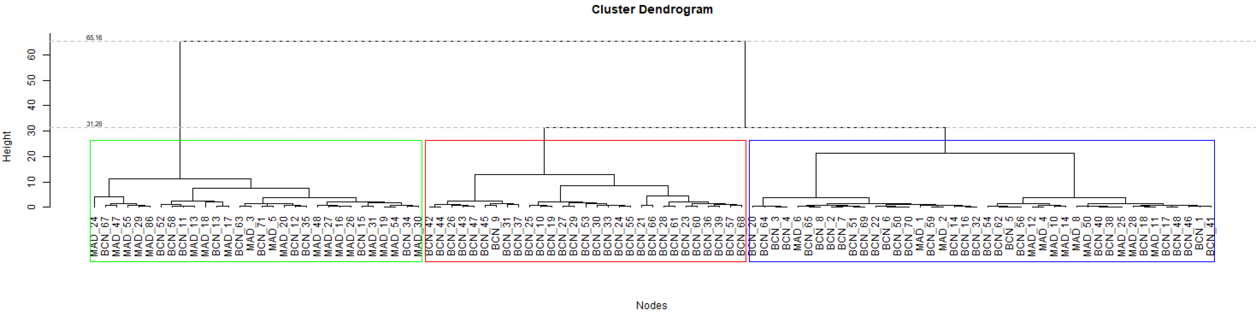
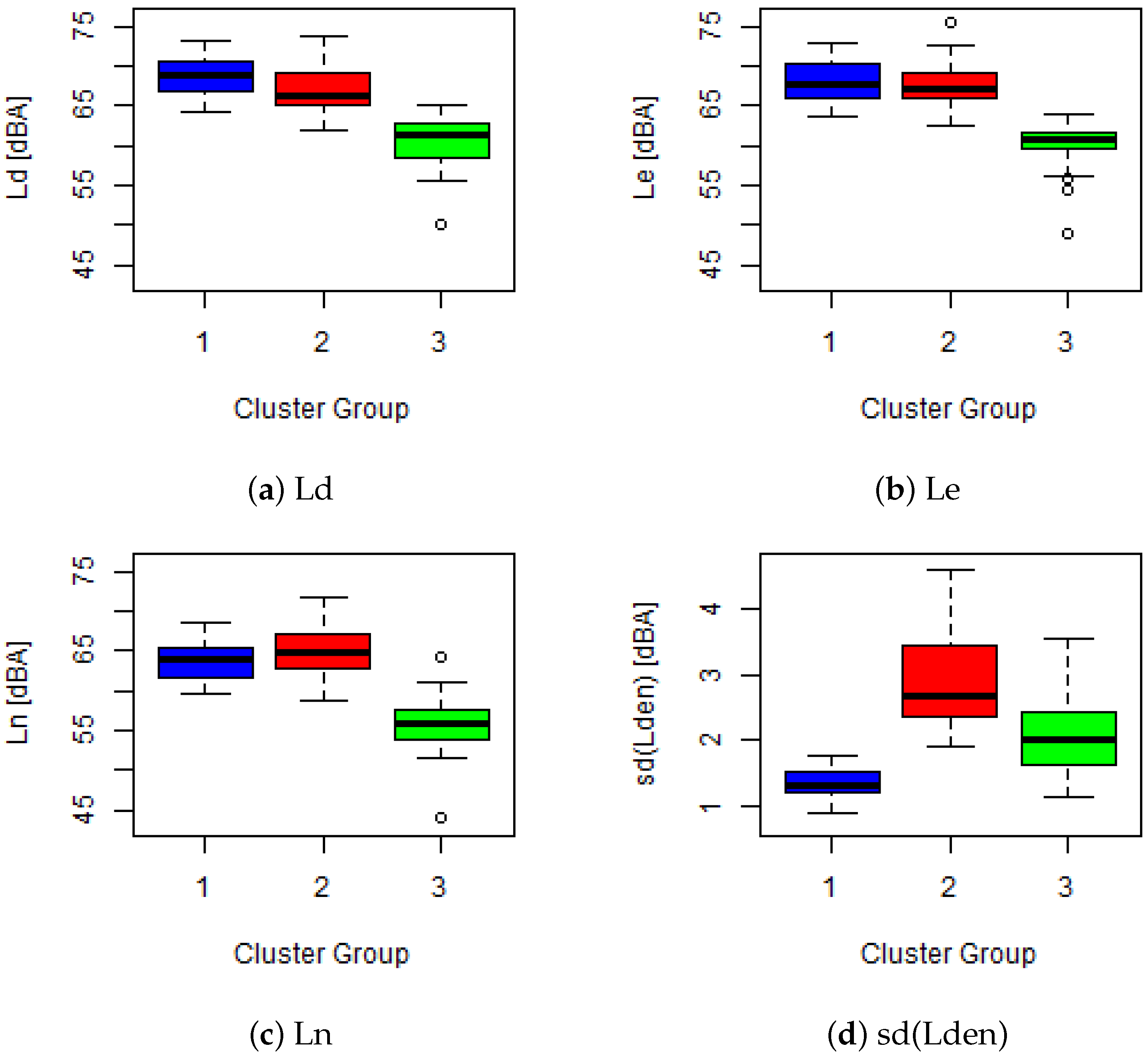
After this first discussion, more details for k = 3 and k = 4 clusters cases are explained below. Applying the Hierarchical Agglomeration algorithm using k = 3, the data are divided into different groups, as it is graphed in a Dendogram in Figure 2. This Figure 2 shows the three main patterns that the algorithm has identified. To study the behavior of these three clusters, four box-plots graphs are shown in Figure 3, corresponding to the parameters used for the training phase, $L_{\mathrm{d}2019}$, $L_{\mathrm{e}2019}$, $L_{\mathrm{n}2019}$ and $s{d}_{2019}$($L_{\mathrm{den}1d}$). It can be observed in Figure 3 that, the first cluster is related to the nodes with high sound pressure levels during the day and evening period, medium sound pressure levels during the night, and the lowest standard deviation of the three clusters, to sum up, there are 42 nodes with a stable and high noise level. The second cluster includes 29 nodes, and presents high sound pressure levels during the three periods reaching maximum noise level values, in addition to the highest standard deviation, in other words, the variation over the mean is high. Finally, the third cluster includes 30 nodes with the lowest sound pressure level during all periods. Moreover, its standard deviation is at an intermediate value between the two other clusters.

A summary of the three discovered clusters obtained with federated data is presented in

Table 6. Size and centroid of clusters using data collected during 2019 for $k=3$ Hierarchical Agglomeration clustering.

Cluster	${\mathit{L}}_{\mathbf{d}2019}$	${\mathit{L}}_{\mathbf{e}2019}$	${\mathit{L}}_{\mathbf{n}2019}$	${\mathit{s}\mathit{d}}_{2019}$(${\mathit{L}}_{\mathbf{den}1\mathit{d}}$)	Size	#MAD 1	#BCN 1	Color
1	68.7	68.2	63.6	1.36	42	12	30	blue
2	67.0	67.7	65.1	2.93	29	0	29	red
3	60.5	60.0	55.7	2.08	30	19	11	green

¹ Abbreviations: MAD Madrid Stations, BCN Barcelona Stations.

in which the number of nodes per city is broken down together with the centroid of each acoustics parameter.

It is remarkable that, as can be seen in Table 6, cluster number 2 only contains nodes belonging to Barcelona city, suggesting that this type of behavior is specific to this city. Moreover, the relative proportion of Madrid’s nodes in cluster number 1 is lower than in cluster number 3, showing that Madrid has nodes with lower sound pressure levels on average than Barcelona.

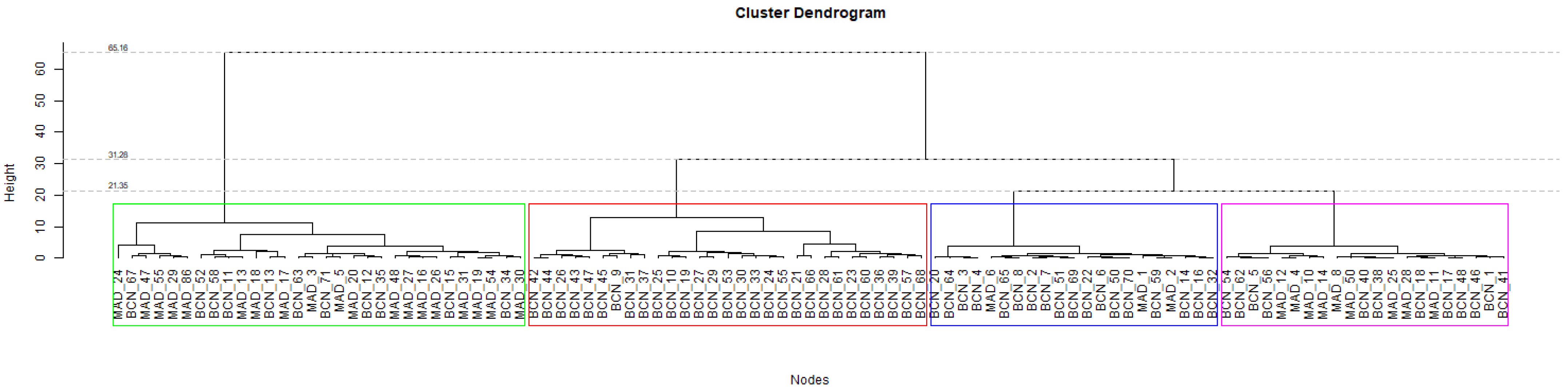
Now, Hierarchical Agglomeration is applied for k = 4 clusters. Figure 4 shows that previous cluster 1 (blue) with 42 nodes, obtained with k = 3, is split into two groups with 21 nodes each (blue and magenta).

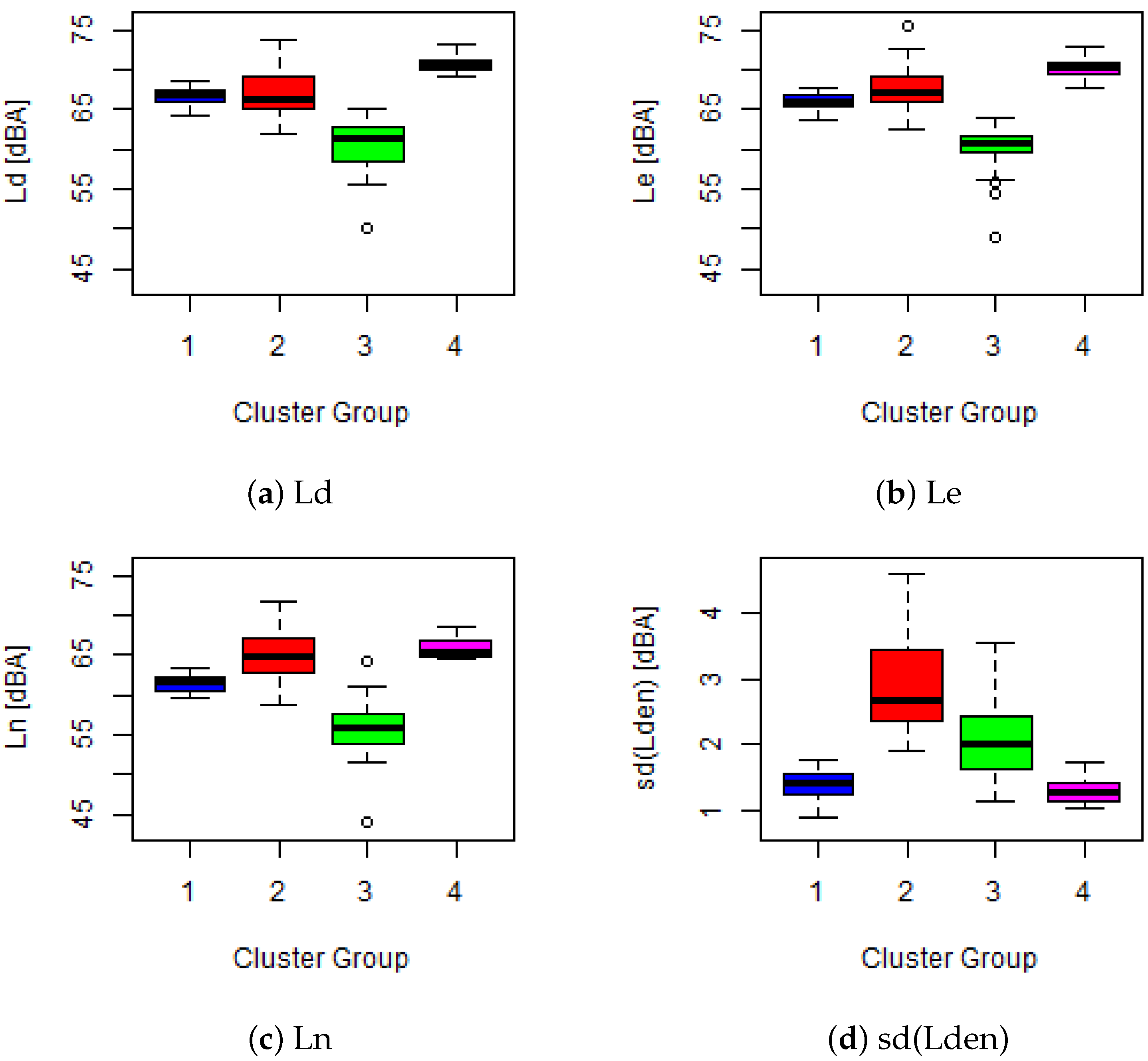
As it can be observed in the boxplots in Figure 5, the new blue cluster presents a lower sound pressure level than magenta and red, with a significant reduction in level during the night period. However, the new magenta cluster is the one with the highest sound pressure level and the lowest variance of the 4 clusters. In this case, the red cluster has the highest standard deviation.

Table 7. Size and centroid of clusters using data collected during 2019 for $k=4$ Hierarchical Agglomeration clustering.

Cluster	${\mathit{L}}_{\mathbf{d}2019}$	${\mathit{L}}_{\mathbf{e}2019}$	${\mathit{L}}_{\mathbf{n}2019}$	${\mathit{s}\mathit{d}}_{2019}$(${\mathit{L}}_{\mathbf{den}1\mathit{d}}$)	Size	#MAD 1	#BCN 1	Color
1	66.7	66.0	61.5	1.41	21	9	12	blue
2	67.0	67.7	65.1	2.93	29	0	29	red
3	60.5	60.0	55.7	2.08	30	19	11	green
4	70.7	70.4	65.8	1.31	21	3	18	magenta

¹ Abbreviations: MAD Madrid Stations, BCN Barcelona Stations.

summarizes the clusters showing distribution and centroids. As in the previous case, Madrid only presents three of four behaviors, explaining the outputs of the Silhouette Width metric of k = 3 for Madrid data, and $k=4$ for both Barcelona and federated data, see details in Section 3.

Regarding the selection based on the Dunn index, from a noise pollution management perspective, it is neither useful nor easy to handle 12 clusters with only 2.6 nodes on average in Madrid and 5.8 nodes on average in Barcelona. This requires establishing 12 strategies with their associated action plans, therefore K-means for k = 12 is discarded from this analysis.

Another way to compare the results is using an external clustering validity index. If federated data clusters are considered the ground truth partition of the nodes, external evaluation metrics can select the more appropriate clustering completed in isolation. The Chi index is an external clustering validity index based on the chi-squared statistical test, very competitive that, on average, beats other external evaluation metrics [49]. The Chi index takes a value in [0, 2], where 0 is given by the worst clustering solution, and 2 is the best value that the Chi index can achieve. Chi index results are clear to read, require no further interpretation, and help to select the optimal number of clusters based on the ground truth class.

Table 8. Comparison Federated Data k = 3 Hierarchical Agglomeration (in rows) with isolation BCN ¹ or MAD ¹ data clustering optimal models.

	(a) BCN 1 Data k = 3 K-Means			(b) MAD 1 Data k = 3 K-Means
Cluster	1	2	3	1	2	3
1	25	5	0	0	0	12
2	10	10	9	0	0	0
3	0	11	0	5	13	1
	Chi index: 0.759			Chi index: 1.777
	(c) BCN 1 Datak= 4 K-means				(d) MAD 1 Datak= 2 Hierarchical
Cluster	1	2	3	4	1	2
1	18	12	0	0	12	0
2	5	14	9	1	0	0
3	0	1	0	10	9	10
	Chi index: 1.104				Chi index: 0.714

¹ Abbreviations: MAD Madrid Stations, BCN Barcelona Stations.

shows results in cross tables a comparison between the k = 3 Hierarchical Agglomeration clustering considering the federated dataset, in rows, and the optimal cluster models trained considering isolated datasets, which are k = 3 and k = 4 K-means for Barcelona dataset, upper-left and lower-left, respectively, and k = 3 K-means and k = 2. Hierarchical for Madrid dataset, upper-right and lower-right, respectively. For instance, the upper-left cross table shows the distribution of the Barcelona nodes considering k = 3 K-means using federated data in rows and $k=3$ K-means Barcelona data in columns, so the number 9 in the second row and third columns represents the number of Barcelona nodes belonging to cluster number 2 in k = 3 K-means model using federated data and belonging to cluster number 3 in k = 3 K-means model using Barcelona data.

For Barcelona city, the federated dataset improves the result of the clustering compared with the Barcelona isolation data (1.104 maximum Chi index). So k = 4 K-means clustering is the best algorithm for Barcelona city based on the federated dataset clusters (chi index 1.104 versus Chi index 0.759 for k = 3 K-means algorithm). For Madrid city, the k = 3 K-means clustering is the best algorithm with a Chi index of 1.777 (compare to k = 2 Hierarchical Agglomeration with 0.714 Chi index). In this case, a smaller improvement has been made with the federated dataset (0.223 = 2 − 1.777), concluding that the clustering created with Madrid data in isolation gives almost the same information that the one created with the federated dataset.

4. Conclusions

Noise pollution is a major concern in cities around the world and wireless acoustic sensor networks are being deployed to acquire information about sound pressure level in many locations and during long-term. Sharing data between administrations in a big data infrastructure, as the EU commission is promoting, can help to obtain better insights and create a common framework. Machine Learning techniques are being applied to learn and analyze these datasets.

In this work, several machine learning clustering techniques have been applied to identify different acoustic environment patterns from sound pressure level datasets. A comparison of clustering techniques for modeling acoustic data from wireless acoustic sensor networks of the cities of Barcelona and Madrid (Spain) has been made. This evaluation has been performed using isolated data and federated data and three parameters as metrics: Connectivity, Dunn index, and Silhouette Width.

From the results, it is observed that both Hierarchical Agglomeration clustering and K-means have the best performance, in both federated and non-federated data. Therefore, they are the more suitable algorithms to fit environmental acoustics parameters, such as sound pressure levels during different periods of the day.

In general, the Connectivity and Silhouette indexes tend to select a low amount of clusters, whereas the Dunn index suggests a large number of groups. Regarding the use case of noise monitoring and management of the noise plans, a small amount of clusters is recommended, therefore the Connectivity or Silhouette index has been used to select the optimal clustering algorithm.

An external clustering validity index, the Chi index, has been also calculated, obtaining insight into the relevance of using federated data to do the clustering. More datasets will be incorporated in future works to further analyze the benefits of using federated datasets instead of isolated datasets.

It has been shown that these techniques can help the local administrations to dynamically detect different patterns of sound pressure level behavior and update the definition of acoustic zones. Moreover, this information can be publicly shared with citizens to know about the acoustic typology of the area in which they live or are planning to buy a house, allowing them better decisions.

Possible future work can continue this research along the following lines:

1.

Design a methodology for monitoring the evolution of the acoustic zones to be able to measure the effect of the actions carried out by the consistories included in their action plans.

2.

Create an acoustic open data spaces for federated data to identify common clusters.

3.

Develop an algorithm to identify the cluster in which belongs to a city spot considering only a small sample of data.