Identification of Dynamic Parameters and Frequency Response Properties of Active Hydraulic Mount with Oscillating Coil Actuator: Theory and Experiment

Abstract

Active hydraulic mounts (AHMs) provide an effective solution for refining ride comfort noise and vibration in passenger cars. AHMs with inertia tracks, decoupler membranes, and oscillating coil actuators (AHM-IT-DM-OCAs) have been extensively studied owing to their compact structures and strong damping characteristics in the low-frequency band. This study focuses on the full parameter identification based on the distinct features of external dynamics, which can be used to obtain an accurate and reliable estimate of the transfer functions required for active control algorithms. A lumped parameter model was established for the AHM-IT-DM-OCAs, and the analytical frequency bands were defined by the two resonance frequencies of the fluid channel and actuator mover. Methods for nonlinear model simplification were proposed in different bands and verified theoretically. Based on the simplified models, the distinct features of the active and passive dynamics are successively revealed, which include three resonances and seven horizontal segments. Subsequently, a series of experimental studies on the distinct features were carried out, which agreed well with the theoretical results. However, owing to the limitations of the test equipment and fixture modalities, only the distinct features of one fixed point, two resonance peaks, and three horizontal segments can be used for parameter identification. Based on the validated distinct features, a procedure for full parameter identification is proposed, and all six key parameters are identified. The obtained results showed good consistency and rationality, indicating that this approach can be used for the transfer function estimation of the primary and secondary paths of the AHM-IT-DM-OCAs.

1. Introduction

Mounts are elastic connections between the powertrain and body/chassis. They are key components for isolating and attenuating the vibration of the powertrain and reducing structurally borne noise. The passive hydraulic engine mount with an inertia track and decoupler membrane (PHM-IT-DM) has been extensively investigated because of its excellent performance, which can provide high stiffness and strong damping in the low-frequency band. Expanding upon the advantages of strong damping in the low-frequency band of the PHM-IT-DM, an active hydraulic mount with an inertia track, decoupler membrane, and oscillating coil actuator (AHM-IT-DM-OCA) has been studied and applied to refine noise and vibration with an active force to cancel the force transmitted to the vehicle body through the primary path. Compared with active hydraulic mounts with magnetostrictive actuators [1], piezoelectric actuators [2], and shape memory alloys [3], the AHM-IT-DM-OCA has the advantages of a compact structure, low energy consumption, sensitive response, large actuating displacement, and linear actuating force.

The investigation of active hydraulic mounts (AHMs) involves three aspects: the model, its parameters, and control algorithm [4,5]. The model and its parameters form the basis of the control algorithm. Active and passive hydraulic mounts are generally modeled using a lumped-parameter model. The accuracy of the parameters is essential for controlling the stability and capability of an algorithm. Methods for acquiring parameters include numerical calculations, direct testing, and parameter identification.

The numerical calculation methods are based on virtual prototypes. The conventional method is the finite element method (FEM), which focuses on the super-elastic constitutive of rubber [6,7] and multiple physics coupling fields [8,9]. Considering the limitations of convergence and accuracy of fluid–solid interaction (FSI) at high frequencies, FEM with FSI is always performed in the lower frequency band. Direct testing methods [10,11,12] are generally used to study specific components when a physical prototype exists. Special fixtures or test rigs are required for the parameter acquisition of different components, such as the main rubber spring, upper fluid chambers, inertia tracks, and decoupler membranes. Therefore, direct testing is time consuming and labor intensive. Moreover, mount element-level tests cannot accurately reflect the operating boundary condition in the way assembly level tests can. Therefore, direct testing is inappropriate for identifying the key parameters of the decoupler membrane attached to the actuator, which significantly influences the accuracy of the model for active control.

Parameter identification methods are based on the external dynamics of the mount assembly when a physical prototype is available. Depending on whether the acquired parameters have a specific physical meaning, parameter identification can be performed based on curve fitting or distinct features.

Curve fitting, which does not require physical meaning, can be carried out based on the Freudenberg hydromount equations [13] and quadratic polynomials [14,15] to simulate the dynamic behaviors. Focusing on frequency-variant dynamics, the curve fitting method can be applied in the low- and high-frequency bands using two different sets of parameters [16,17]. Regardless of whether the mathematical model is linear or nonlinear, curve fitting can achieve good agreement with the experimental results [18].

Parameter identification methods based on the distinct features of dynamics identify parameters based on the relationship between external dynamics and internal physical parameters, focusing on the physical meanings of the parameters. For hydraulic engine mounts, the key physical parameters mainly include the bulk stiffness, equivalent piston area, and natural frequency, which can be identified by a fixed point and a horizontal segment [19,20,21]. The above-mentioned studies for parameter identification mainly focused on distinct features in the mid- and low-frequency bands before and after fluid channel resonance. Only the bulk stiffness of the upper fluid chamber, which is a coupling parameter, and equivalent piston area of the main rubber spring are involved. For the AHM-IT-DM-OCA, a mount with more physical parameters has a conventional fluid channel and an actuator mover whose modal frequency exceeds 200 Hz. Therefore, all physical parameters of the decoupler membrane with an actuator mover must be systematically identified. It is necessary and significant that further investigations on parameter identification by distinct features should be carried out in mid- and high-frequency bands.

The discussion focuses on the identification of all key parameters based on a thorough analysis of the distinct features of the AHM-IT-DM-OCA. A nonlinear model involving all key parameters is established. Moreover, the analytical bands are defined by the natural frequency of the fluid channel and actuator mover; thus, methods for simplifying the nonlinear model in different bands are carried out. Subsequently, the distinct features of the dynamics are analyzed, particularly the active dynamics. The relationships between the distinct features and key parameters were simultaneously explored. Experimental research was carried out to validate the consistency of the distinct features between the analysis and test results. Finally, a detailed procedure for all key parameter identification is proposed, which is successively stated from passive dynamics to active dynamics.

2. Model of an Active Hydraulic Mount and Frequency Band Definition

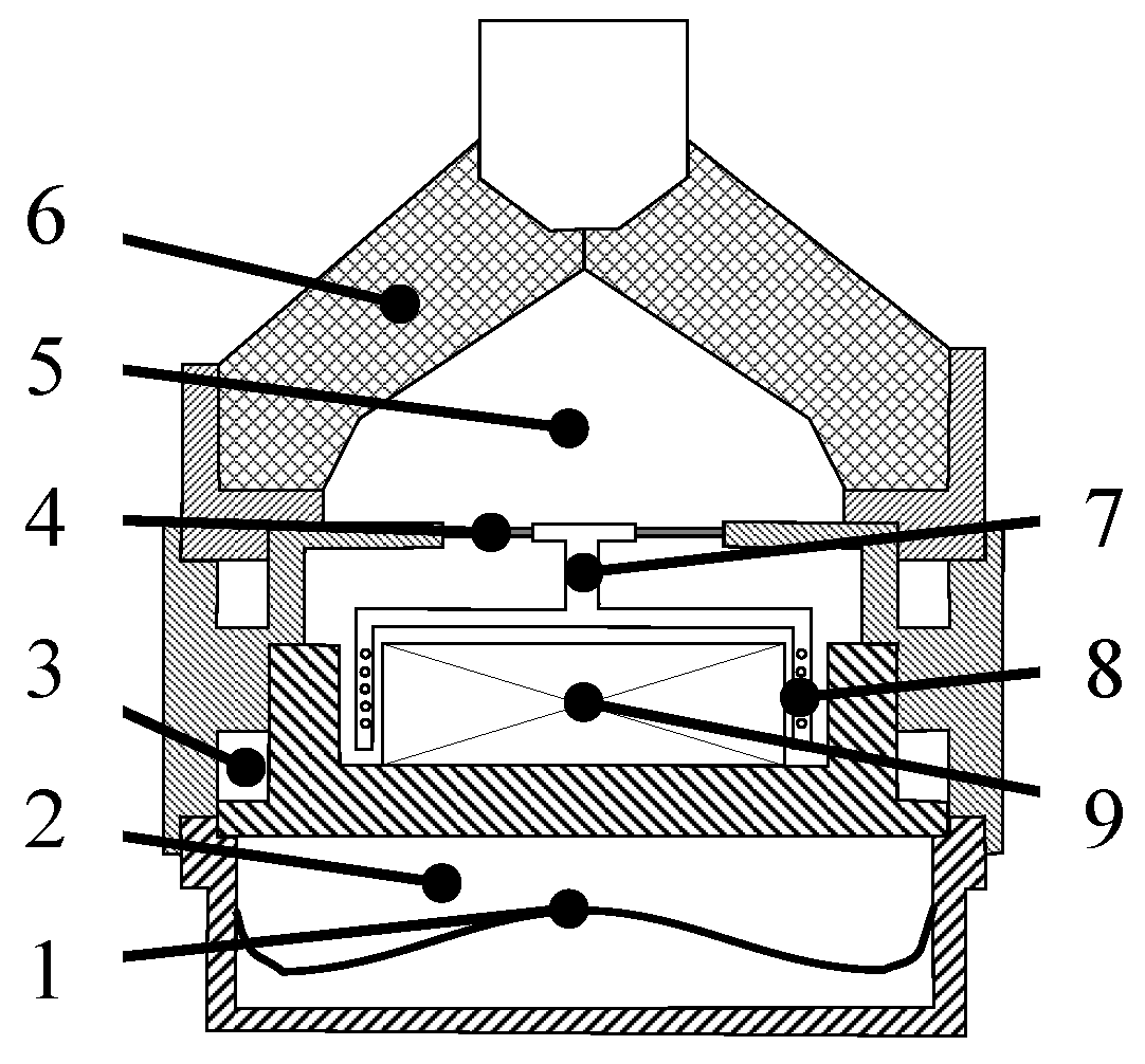
2.1. Model of the Active Hydraulic Mount with Oscillating Coil Actuator

A schematic of the AHM-IT-DM-OCA is shown in Figure 1. The upper end is connected to the engine, and the lower end is connected to the vehicle body or chassis. The coil bobbin was rigidly connected to the skeleton of the decoupler membrane, which was regarded as an actuator mover. Alternating current (AC) power is applied to the coil, and the coil oscillates under an alternating ampere force in the constant magnetic field of a permanent magnet. The ampere force is the active force controlled by the amplitude and frequency of the AC. The resultant force acting on the vehicle body consists of the active force transmitted to the vehicle body through the secondary path and the force transmitted from the engine to the vehicle body through the primary path, which can be controlled such that it remains zero under ideal conditions.

The variables for the lumped parameter model of the AHM-IT-DM-OCA are shown as follows. Referring to the hydraulic mount mechanical models [4,16], a lumped parameter mechanical model for the AHM-IT-DM-OCA was established, as shown in Figure 2. The displacement on the engine side is y₁, and the corresponding reaction force f₁ is the force acting on the mount. The displacement of the fluid in the horizontal fluid channel is y₂, and the mover displacement is y₃. The displacement on the chassis side is y₅, and the force transmitted to the chassis side is f₅. The pressure fluctuations of the upper and lower fluid chambers relative to the static state are p₁ and p₂, respectively. The active force of the actuator is f_a.

The parameters for the lumped parameter model of the AHM-IT-DM-OCA are shown as follows. The mass on the engine side is denoted by m₁, the mass of fluid in the inertia track is denoted by m₂ and the mass of the actuator mover with the attached fluid is denoted by m₃. The in-phase vertical dynamic stiffness, viscous damping, and equivalent piston area of the main rubber spring are denoted by k₁, c₁, and A₁, respectively. The linear stiffness, viscous damping, and equivalent piston area of the decoupler membrane are denoted by k₃, c₃, and A₃, respectively. The bulk stiffnesses of the main rubber spring, rubber bellow, and decoupler membrane are K₁, K₂, and K₃, respectively. The bulk stiffness K₂ of the lower fluid chamber enclosed by the wrinkled rubber bellows was several orders of magnitude smaller than K₁. Thus, K₂ = 0, and the pressure fluctuation in the lower fluid chamber can be ignored by assuming p₂ = 0 [22,23]. The relationship between linear stiffness k₃ and bulk stiffness K₃ can be expressed by Equation (1).

$$A_3^2{K}_3=k_3$$

(1)

The length, cross-sectional area, and hydraulic diameter of the inertial track are denoted by l₂, A₂, and d₂, respectively. The loss factor of the fluid flowing along the inertia track can be expressed as ξ_l2 [24]. The local loss factor of the fluid flowing at the entrance and outlet is given as ξ_d2.

Eight key parameters of the main rubber spring, decoupler membrane and actuator mover need to be identified. Parameters k₁ and c₁ for the main rubber spring can be acquired directly from the test results. Therefore, six key parameters (K₁, A₁, K₃, A₃, m₃, and c₃) that are independent of each other must be identified by distinct features of the dynamics.

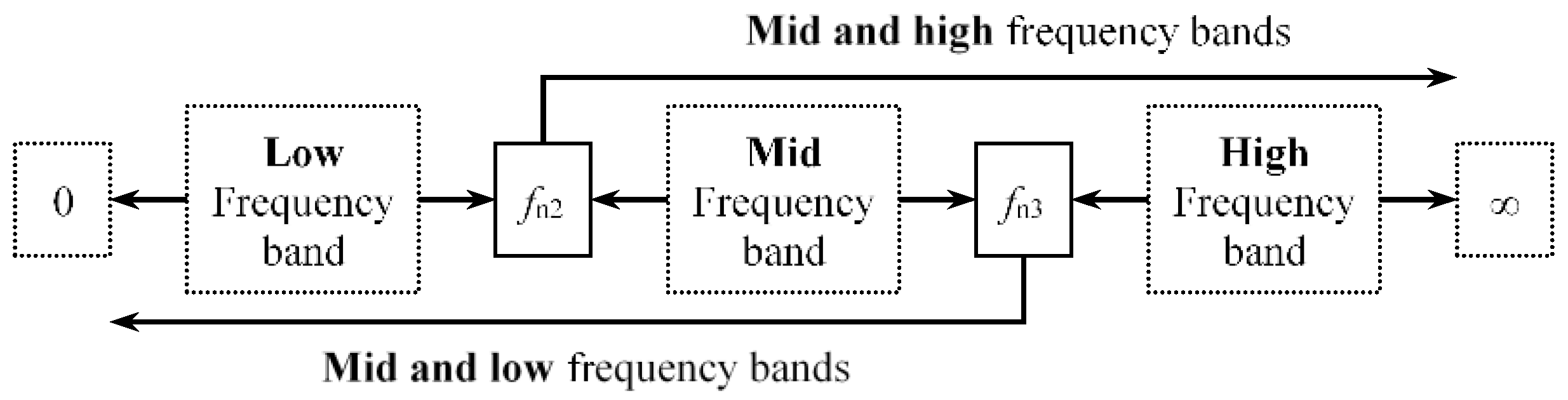
2.2. Dynamics of the Active Hydraulic Mount and Frequency Band Definition

An AHM has active and passive dynamics. Distinct features of the dynamics were studied to identify the key parameters. The study of the distinct features of passive dynamics lays the foundation for model simplification and decoupling of key parameters based on active dynamics.

The passive dynamics refer to frequency response functions (FRFs) with the chassis side fixed and the actuator powered off. The input of the FRFs is the engine-side displacement, and the outputs are the reaction force of the engine side and the force transmitted to the chassis side. They are called the drive- and cross-point dynamics by definition. Cross-point dynamics are the primary path-transfer functions in the control of an AHM. The active dynamics refer to FRFs with the engine and chassis sides fixed. The input is the actuator current, and the outputs are the reaction force of the engine side and the force transmitted to the chassis side. The active dynamics from the actuator current to the force transmitted to the chassis side are the secondary path transfer functions in the control of the AHM-IT-DM-OCA.

The AHM-IT-DM-OCA involves the resonance of two subsystems: the fluid channel and the mover. Experimental studies have shown that the natural frequency f_n3 of an actuator mover in the fluid-filled state is typically greater than 200 Hz, which is much higher than the natural frequency f_n2 of the fluid channel (typically less than 20 Hz). Research on f_n2 has been thoroughly conducted and can be expressed as Equation (2). For the forced vibrations of a 1-DOF system, the natural frequency f_n3 of the actuator mover in the fluid-filled state can be expressed using Equation (3). Since the two natural frequencies are far apart, the analytical bands are divided into low-, mid-, and high-frequency bands to simplify the inertia and damping forces in different frequency bands, as shown in Figure 3.

$$f_{\mathrm{n}2}=\frac{1}{2\pi }\sqrt{\frac{A_2}{\rho l_2}{K}_{\mathrm{u}1}}$$

(2)

$$f_{\mathrm{n}3}=\frac{1}{2\pi }\sqrt{\frac{A_3^2\left(K_1+K_3\right)}{m_3}}$$

(3)

where K_u1 is the bulk stiffness of the upper chamber surrounded by the main rubber spring and decoupler membrane and can be expressed as Equation (4) [22,23]. ρ denotes the density of the fluid in the hydraulic mount.

$$\frac{1}{K_{\mathrm{u}1}}=\frac{1}{K_1}+\frac{1}{K_3}$$

(4)

Mathematical models were established and simplified for different frequency bands for active and passive dynamics. Nonlinear and linear mathematical models for mid- and low-frequency bands were constructed to investigate the distinct features of the dynamics, which can be expressed by the following equation:

$$k^{\ast }=k\left(\cos \phi +j\sin \phi \right)=k^{\prime }+j{k}^{″}=k^{\prime }+j\omega c$$

(5)

where k* is the dynamic stiffness, k is the dynamic stiffness modulus, φ is the loss angle, k′ is the in-phase dynamic stiffness, k″ is the out-of-phase dynamic stiffness, and c is the viscous damping.

3. Mathematical Model Simplification and Distinct Features of Passive Dynamics

Nonlinear mathematical models of AHM-IT-DM-OCA are established in this section. Subsequently, the passive dynamics and distinct features of the electromagnetic actuator powered off were studied. The conventional method for identifying the key parameters of the main rubber spring and upper chamber is briefly introduced. Furthermore, the method for simplifying the nonlinear model to a linear model in mid- and high-frequency bands is detailed. The rationality of the method is proven by the consistency of distinct features in the mid-frequency band inferred by two different models.

3.1. Mathematical Model Simplification in Different Frequency Bands

In the analysis of passive dynamics, the engine-side displacement y₁ is the input excitation, and the engine-side reaction force f₁ and transmitted force f₅ to the chassis side are the outputs.

Based on the mechanical model for the AHM-IT-DM-OCA shown in Figure 2, by setting m₁ = 0, y₅ = 0, and f_a = 0, the nonlinear mathematical model for passive dynamics can be expressed as Equation (6). The equations are, in order, the Bernoulli equation for fluid flowing in the inertia track [24], differential equation for the mover, fluid continuity equation, equilibrium equation for engine-side reaction forces f₁, and transmitted force f₅ to the chassis side.

As a significant distinct feature for parameter identification of passive hydraulic mounts, the fixed point related to the inertia track has been thoroughly studied. The studies [25] involve mid- and low-frequency bands, which refer to f << f_n3.

For the analysis in the mid- and low-frequency bands, simplification of the model can be carried out as follows: referring to the mechanical vibration theory [26], under excitation with frequency f << f_n3 in the mid- and low-frequency bands, the mover displacement y₃ is almost in phase with the excitation, and the excitation force is mainly balanced by the elastic restoring force. In this case, the inertia and damping force [4,16,26,27] can be neglected. Therefore, the nonlinear model in Equation (6) for passive dynamics in the mid- and low-frequency bands can be simplified by eliminating intermediate variables p₁ and y₃. The nonlinear model can be expressed using Equation (7).

$$\{\begin{array}{l} \rho l_2{\ddot{y}}_2+\frac{1}{2}\rho \left({\xi }_{l_2}+{\xi }_{d_2}\right)\left|{\dot{y}}_2\right|{\dot{y}}_2=-p_1\\ m_3{\ddot{y}}_3+c_3{\dot{y}}_3+k_3{y}_3+A_3{p}_1=0\\ A_2{y}_2+A_3{y}_3=A_1{y}_1+p_1/K_1\\ f_1=c_1{\dot{y}}_1+k_1{y}_1-A_1{p}_1\\ f_5=c_1{\dot{y}}_1+k_1{y}_1+c_3{\dot{y}}_3+k_3{y}_3-\left(A_1-A_3\right)p_1\\ \hspace{0.17em}\hspace{0.17em}\hspace{0.17em}=f_1-m_3{\ddot{y}}_3\end{array}$$

(6)

$$\{\begin{array}{l}{\ddot{y}}_2+\left(\frac{32\mu }{\rho d_2^2}+\frac{{\xi }_{d_2}}{2l_2}\left|{\dot{y}}_2\right|\right){\dot{y}}_2+\frac{A_2{K}_{\mathrm{u}1}}{\rho l_2}{y}_2=\frac{A_1{K}_{\mathrm{u}1}}{\rho l_2}{y}_1\\ f_5=f_1=c_1{\dot{y}}_1+k_1{y}_1+A_1^2{K}_{\mathrm{u}1}{y}_1-A_1{A}_2{K}_{\mathrm{u}1}{y}_2\end{array}$$

(7)

Experiments and numerical simulations [23] have shown that, under the excitation of harmonic displacement y₁, the excitation and responses can be expressed as follows:

$$y_1=Y_1{e}^{j\omega t},\hspace{1em}{y}_2=Y_2{e}^{j(\omega t-{\phi }_2)},\hspace{1em}{f}_1=f_5=F_1{e}^{j\omega t}=F_5{e}^{j\omega t}$$

(8)

where Y₁ denotes the excitation displacement amplitude, Y₂ is the response amplitude of the inertia fluid displacement, φ₂ is the loss angle of y₂ with respect to y₁, and F₁ and F₅ are the drive point and cross-point response force amplitudes, respectively.

For the analysis in the mid- and high-frequency bands, the simplification method can be carried out as follows: according to the principle of equivalent energy [26], the FRF of Y₁–Y₂ [22] can be expressed as Equation (9). This indicates that the fluid motion in the inertia track can be ignored at frequencies above the fluid channel resonance frequency f_n2. Therefore, the nonlinear factors related to the inertia track are not considered to clearly study the distinct features related to the decoupler membrane in the mid- and high-frequency bands. When f >> f_n2, the linear model can be expressed as Equation (10) by setting y₂ = 0 and simplifying Equation (6).

$$\begin{array}{l}{H}_2=\frac{Y_2}{Y_1}{e}^{-j{\phi }_2}=\frac{A_1}{A_2}\frac{1}{1-{\lambda }^2+j\left(C\lambda /{\omega }_{\mathrm{n}2}+D{Y}_2{\lambda }^2\right)}\\ C=32\mu /\rho d_2^2,\hspace{1em}D=4{\xi }_{d_2}/3\pi l_2,\hspace{1em}\lambda ={\lambda }_2=f/f_{\mathrm{n}2}\end{array}$$

(9)

$$\{\begin{array}{l}{m}_3{\ddot{y}}_3+c_3{\dot{y}}_3+k_3{y}_3+A_3{p}_1=0\\ A_3{y}_3=A_1{y}_1+p_1/K_1\\ f_1=c_1{\dot{y}}_1+k_1{y}_1-A_1{p}_1\\ f_5=c_1{\dot{y}}_1+k_1{y}_1+c_3{\dot{y}}_3+k_3{y}_3-\left(A_1-A_3\right)p_1\\ =f_1-m_3{\ddot{y}}_3\end{array}$$

(10)

3.2. Distinct Features of Passive Dynamics and Verification for Model Simplification Method

In the mid-and low-frequency bands, the passive dynamics of the AHM-IT-DM-OCA have features similar to those of a conventional hydraulic engine mount, which is essentially caused by the inertia track. The significant distinct feature of the fixed point has been thoroughly studied and can be obtained through tests under excitation with different amplitudes. The feature of constant dynamics in the mid-frequency band is named as the 1st horizontal segment.

The fixed point f_R and 1st horizontal segment ${k^{\prime }}_{\infty ,1}$, which can be inferred from the nonlinear model in Equation (7) can be expressed as Equation (11). These features can be applied to identify the equivalent piston area A₁ of the main rubber spring and bulk stiffness K_u1 of the upper chamber. It should be noted that there were no differences between the drive-point and cross-point dynamics when f << f_n3.

$$f_{\mathrm{n}2}=f_R\hspace{0.17em},\hspace{1em}{k^{\prime }}_{\infty ,1}=k_1+A_1^2{K}_{\mathrm{u}1}$$

(11)

In the mid- and high-frequency bands, distinct features can be inferred based on the linear model shown in Equation (10). It should be noted that the inertial force of m₃ cannot be ignored; thus, f₁ and f₅ are no longer the same. Therefore, the drive-point $k_{11}^{*}$ and cross-point $k_{51}^{*}$ passive dynamic stiffnesses can be expressed by Equation (12). Subsequently, the dynamic stiffness in-phase can be obtained.

$$\begin{array}{c}{k}_{11}^{*}=\frac{F_1}{Y_1}=\left(k_1+A_1^2{K}_1\right)+j\omega c_1-\frac{A_1^2{K}_1^2}{K_1+K_3}\frac{1}{\left(1-{\lambda }^2+j2{\xi }_3\lambda \right)}\\ k_{51}^{*}=\frac{F_5}{Y_1}=k_1+A_1^2{K}_1+A_1{A}_3{K}_1\frac{\left({\lambda }^2-G\right)\left(1-{\lambda }^2\right)}{{\left(1-{\lambda }^2\right)}^2+{\left(2{\xi }_3\lambda \right)}^2}\\ +j\left[\omega c_1-A_1{A}_3{K}_1\frac{2{\xi }_3\lambda \left({\lambda }^2-G\right)}{{\left(1-{\lambda }^2\right)}^2+{\left(2{\xi }_3\lambda \right)}^2}\right]\end{array}$$

(12)

where λ, ξ₃ and G can be expressed as follow:

$$\lambda ={\lambda }_3=\frac{\omega }{{\omega }_{\mathrm{n}3}}=\frac{f}{f_{\mathrm{n}3}}\hspace{0.17em},\hspace{1em}{\xi }_3=\frac{c_3}{2m_3{\omega }_{\mathrm{n}3}}=\frac{c_3}{2\sqrt{m_3{A}_3^2\left(K_1+K_3\right)}}\hspace{0.17em},\hspace{1em}G=\frac{A_1{K}_1}{A_3\left(K_1+K_3\right)}=\frac{A_1{K}_{\mathrm{u}1}}{A_3{K}_3}$$

In the mid-frequency band, the frequency ratio λ can be zero because f << f_n3.

Subsequently, drive point $k_{11,0}^{\prime }$ and cross point $k_{51,0}^{\prime }$ dynamic stiffness in-phase in the high-frequency band can be expressed by Equation (13). It should be noted that $k_{11,0}^{\prime }$ and $k_{51,0}^{\prime }$ are equal to the 1st horizontal segment, which is obtained by the nonlinear model, even though f₁ and f₅ are different from each other in the linear mathematical model. The consistency of the 1st horizontal segment obtained by nonlinear and linear models at mid-frequency indicates that the method to achieve a linear model by removing the nonlinear factors is feasible and rational. Therefore, the model simplification method can be verified and applied to study the distinct features of the active dynamics and parameter identification.

$${k^{\prime }}_{11,0}={k^{\prime }}_{51,0}=k_1+A_1^2{K}_{\mathrm{u}1}={k^{\prime }}_{\infty ,1}$$

(13)

In the high-frequency band, the frequency ratio λ can be ∞ because f >> f_n3.

Furthermore, drive point $k_{11,\infty }^{\prime }$ and cross point $k_{51,\infty }^{\prime }$ dynamic stiffness in-phase in the high-frequency band can be expressed by Equation (14). $k_{11,\infty }^{\prime }$ and $k_{51,\infty }^{\prime }$ are denoted as $k_{\infty ,2}^{\prime }$ and $k_{\infty ,3}^{\prime }$, respectively, which are constant in the high-frequency band. Therefore, $k_{\infty ,2}^{\prime }$ is named the 2nd horizontal segment, and $k_{\infty ,3}^{\prime }$ is named the 3rd horizontal segment. They are identified as the distinct features of passive dynamics obtained by the linear mathematical model.

$$k_{11,\infty }^{\prime }=k_1+A_1^2{K}_1=k_{\infty ,2}^{\prime }\hspace{0.17em},\hspace{1em}{k}_{51,\infty }^{\prime }=k_1 +A_1^2{K}_1 -A_1{A}_3{K}_1=k_{\infty ,3}^{\prime }$$

(14)

4. Mathematical Model and Distinct Features of Active Dynamics

In this section, a mathematical model for the active dynamics of the AHM-IT-DM-OCA is established. Subsequently, the dynamics and distinct features with both the engine and chassis sides fixed and only the electromagnetic actuator operating were studied. Moreover, to thoroughly study the distinct features and identify all parameters, the active FRFs in the non-fluid state were studied.

4.1. Mathematical Model of Active Dynamics in Two Different States

With an oscillating coil as the actuator, the linear relationship between the active ampere force f_a(t) and the excitation current i(t) can be expressed as Equation (15).

$$f_{\mathrm{a}}\left(t\right)=Bli\left(t\right)=k_{\mathrm{M}}i\left(t\right)$$

(15)

where B is the magnetic induction intensity, l is the coil length, and k_M is the voice-coil constant.

The model for the active dynamics analysis is based on two different states: a fluid-filled state and a non-fluid state. The input of the dynamics in both states is the actuator current i. For the fluid-filled state, the outputs are the reaction force f₁ and transmitted force f₅. However, for the non-fluid state, the outputs are the mover acceleration ${\ddot{y}}_3$ and transmitted force f₅ to the chassis side.

In the fluid-filled state, because the engine and chassis sides are fixed, and the boundary conditions can be expressed as y₁ = 0 and y₅ = 0 based on the mechanical model shown in Figure 2. The nonlinear mathematical model of the active dynamics can then be obtained using Equation (16).

$$\{\begin{array}{l}\rho l_2{\ddot{y}}_2+\frac{1}{2}\rho \left({\xi }_{l_2}+{\xi }_{d_2}\right)\left|{\dot{y}}_2\right|{\dot{y}}_2=-p_1\\ m_3{\ddot{y}}_3+c_3{\dot{y}}_3+k_3{y}_3+A_3{p}_1=f_{\mathrm{a}}\\ A_2{y}_2+A_3{y}_3=p_1/K_1\\ f_{\mathrm{a}}\left(t\right)=Bli\left(t\right)=k_{\mathrm{M}}i\left(t\right)\\ f_1=-A_1{p}_1\\ f_5=c_3{\dot{y}}_3+k_3{y}_3-\left(A_1-A_3\right)p_1-f_{\mathrm{a}}=f_1-m_3{\ddot{y}}_3\end{array}$$

(16)

$$\{\begin{array}{l}{m}_{3,\mathrm{nof}}{\ddot{y}}_3+c_{3,\mathrm{nof}}{\dot{y}}_3+k_3{y}_3=f_{\mathrm{a}}\\ f_{\mathrm{a}}\left(t\right)=Bli\left(t\right)=k_{\mathrm{M}}i\left(t\right)\\ f_1=0\\ f_5=c_{3,\mathrm{nof}}{\dot{y}}_3+k_3{y}_3-f_{\mathrm{a}}=-m_{3,\mathrm{nof}}{\ddot{y}}_3\end{array}$$

(17)

It should be noted that in the non-fluid state, the AHM-IT-DM-OCA is incomplete and significantly different. First, the mount is not filled with fluid, and the main rubber spring is not compressed. The chassis side is fixed, and there is no force transmitted to the engine side when the actuator is operating; therefore, f₁ = 0. Second, in the non-fluid state, the mover mass and damping are different from those in the fluid-filled state; set model m₃ = m_3,nof and c₃ = c_3,nof. Third, the linear stiffness of the decoupler membrane remains k₃, regardless of whether it is in a non-fluid or fluid-filled state.

Based on the mechanical model shown in Figure 2, setting y₁ = 0 and y₅ = 0, a linear model for the active dynamics of the AHM-IT-DM-OCA in the non-fluid state can be obtained as Equation (17).

4.2. Distinct Features of Active Dynamics in Fluid-Filled State

As discussed in Section 2.2, the natural frequency f_n3 of an actuator mover in a fluid-filled state is typically above 200 Hz. The bands for the distinct feature research of active dynamics are mainly involved in the mid- and high-frequency bands, that is, f >> f_n2. Subsequently, the nonlinear model in Equation (16) can be simplified using the method described in Section 3.1. The inertial track was turned off, and y₂ = 0. The FRFs of the reaction force f₁ and transmitted force f₅ to the actuator current i can be expressed by Equation (18).

$$\begin{array}{c}-\frac{F_1}{I}=\frac{A_1{K}_{\mathrm{u}1}}{A_3{K}_3}{k}_{\mathrm{M}}\cdot \frac{1}{1-{\lambda }^2+j2{\xi }_3\lambda }=\frac{G{k}_{\mathrm{M}}}{1-{\lambda }^2+j2{\xi }_3\lambda }\\ -\frac{F_5}{I}=k_{\mathrm{M}}\cdot \frac{G-{\lambda }^2}{1-{\lambda }^2+j2{\xi }_3\lambda }\hspace{0.17em}\hspace{0.17em},\hspace{1em}\lambda ={\lambda }_3=\frac{\omega }{{\omega }_{\mathrm{n}3}}=\frac{f}{f_{\mathrm{n}3}}\end{array}$$

(18)

In the mid-frequency band, λ can be zero because f << f_n3. Distinct features can be obtained and expressed by Equation (19). It should be noted that the active FRF of f₁ and f₅ in the mid-frequency band are equal to a constant F_i,∞,4, which is referred to as the 4th horizontal segment. Therefore, the coupling parameter A₃K₃ can be identified based on the known parameter k_M and parameters A₁ and K_u1 identified by the distinct features of passive dynamics.

$$-{\frac{F_1}{I}|}_{\lambda \to 0}=-{\frac{F_5}{I}|}_{\lambda \to 0}=\frac{A_1{K}_{\mathrm{u}1}}{A_3{K}_3}{k}_{\mathrm{M}}=F_{i,\infty ,4}$$

(19)

In the high-frequency band, λ can be ∞ because f >> f_n3. Similarly, distinct features can be obtained and expressed by Equation (20). It can be seen that the chassis-side active dynamics are the voice coil constant k_M, which is referred to as the 5th horizontal segment F_i,∞,5. Moreover, the active force reappears on the chassis side at a ratio of 1:1 and is not transmitted to the engine side.

$$-{\frac{F_1}{I}|}_{\lambda \to \infty }=0\hspace{0.17em}\hspace{0.17em},\hspace{1em}-{\frac{F_5}{I}|}_{\lambda \to \infty }=k_{\mathrm{M}}=F_{i,\infty ,5}$$

(20)

At the peak of |−F₁/I|, the distinct features, including the peak value A_p,1, peak frequency f_p,1, and peak frequency ratio λ_p,1, can be expressed as Equation (21). Therefore, parameter ξ₃ can be identified by the known 4th horizontal segment F_i,∞,4. Subsequently, f_n3 can be identified by the distinct features of f_p,1.

$$A_{\mathrm{p},1}={\left|-\frac{F_1}{I}\right|}_{\mathrm{p}}=F_{i,\infty ,4}\cdot \frac{1}{2{\xi }_3\sqrt{1-{\xi }_3^2}}\hspace{0.17em}\hspace{0.17em},\hspace{1em}{\lambda }_{\mathrm{p},1}=\frac{f_{\mathrm{p},1}}{f_{\mathrm{n}3}}=\sqrt{1-2{\xi }_3^2}$$

(21)

4.3. Distinct Features of Active Dynamics in Non-Fluid State

Two coupling parameters, K_u1 and A₃K₃, were identified. However, they still need to be decoupled further. The identification of the linear stiffness of the decoupler membrane k₃ is essential for decoupling these two coupling parameters. The natural frequency of the mover system in the non-fluid state f_n3,nof is different from that in the fluid-filled state, which can be expressed as Equation (22).

$$f_{\mathrm{n}3,\mathrm{nof}}=\frac{1}{2\pi }\sqrt{\frac{k_3}{m_{3,\mathrm{nof}}}}$$

(22)

Since the structure in a non-fluid state is different, the distinct features are related to the resonance of the decoupler membrane and mover system.

According to the linear model in the non-fluid state shown in Equation (17), the FRF of the mover acceleration to the actuator current and the distinct features can be expressed as Equation (23). It should be noted that the distinct features are the mover resonance peak followed by a horizontal segment, which are referred to as the resonance peak A_p,3,nof at the ratio of λ_p,3,nof and the 6th horizontal segment ${\ddot{Y}}_{i,\infty ,6}$. λ_p,3,nof can be expressed using Equation (24).

$$\begin{array}{l}\left|\frac{{\ddot{Y}}_3}{I}\right|=\{\begin{array}{l}\frac{{\ddot{Y}}_{i,\infty ,6}}{2{\xi }_{3,\mathrm{nof}}\sqrt{1-{\xi }_{3,\mathrm{nof}}^2}}=A_{\mathrm{p},3,\mathrm{nof}}\hspace{0.17em},\hspace{0.17em}\hspace{1em}{\lambda }_{3,\mathrm{nof}}={\lambda }_{\mathrm{p},3,\mathrm{nof}}\\ \frac{k_{\mathrm{M}}}{m_{3,\mathrm{nof}}}={\ddot{Y}}_{i,\infty ,6}\hspace{0.17em}, \hspace{0.17em} \hspace{0.17em}{\lambda }_{3,\mathrm{nof}}\to \infty \end{array}\\ \hspace{0.17em}{\lambda }_{3,\mathrm{nof}}=\frac{\omega }{{\omega }_{\mathrm{n}3,\mathrm{nof}}}=\frac{f}{f_{\mathrm{n}3,\mathrm{nof}}}\hspace{0.17em},\hspace{0.17em}\hspace{1em}{\xi }_{3,\mathrm{nof}}=\frac{c_{3,\mathrm{nof}}}{2\sqrt{m_{3,\mathrm{nof}}{k}_3}}\end{array}$$

(23)

$${\lambda }_{\mathrm{p},3,\mathrm{nof}}=\frac{f_{\mathrm{p},3,\mathrm{nof}}}{f_{\mathrm{n}3,\mathrm{nof}}}=\frac{1}{\sqrt{1-2{\xi }_{3,\mathrm{nof}}^2}}$$

(24)

Similarly, distinct features can be obtained for the FRF of the transmitted force f₅ to the actuator current i, as shown in Equation (25). The frequency ratio of the resonance peaks is denoted by λ_p,5,nof. The constant in the high-frequency band is named the 7th horizontal segment F_i,∞,7. If the FRF curves can be obtained accurately and smoothly, the physical parameters m_3,nof, k₃, c_3,nof, and ξ_3,nof can be identified based on the resonance peak A_p,3,nof, the 6th horizontal segment ${\ddot{Y}}_{i,\infty ,6}$, and a known voice coil constant k_M.

$$\left|\frac{F_5}{I}\right|=\{\begin{array}{l}\frac{k_{\mathrm{M}}}{2{\xi }_{3,\mathrm{nof}}\sqrt{1-{\xi }_{3,\mathrm{nof}}^2}}=A_{\mathrm{p},5,\mathrm{nof}}\hspace{0.17em},\hspace{0.17em}\hspace{1em}{\lambda }_{3,\mathrm{nof}}={\lambda }_{\mathrm{p},5,\mathrm{nof}}={\lambda }_{\mathrm{p},3,\mathrm{nof}}\\ k_{\mathrm{M}}=F_{i,\infty ,7}\hspace{0.17em},\hspace{0.17em}\hspace{0.17em}\hspace{0.17em}\hspace{0.17em} {\lambda }_{3,\mathrm{nof}}\to \infty \end{array}$$

(25)

Subsequently, based on the distinct features of the dynamics, all key parameters can be identified. Complete experimental research was conducted to verify the feasibility of the method for all parameters.

5. Experimental Validation and Parameters Identification

In this section, experiments of passive and active dynamics are carried out for the identification of all key parameters, and the detailed procedure is shown in the

Table A1. Parameter identification procedure and obtained results for an AHM-IT-DM-OCA.

Parameters	Data Source or Formula		Values
*: Parameters for the model in Figure 2.			* 1: Italic font for original data; * 2: Regular font for experimental data; * 3: Bold font for identified data.
1. Original data
* 1.1. Fluid density, ρ (kg⋅m−3)			1000.00 *,1
* 1.2. Length of inertia track, l2 (mm)			328.80
* 1.3. Cross-sectional area of inertia track, A2 (mm2)			92.50
* 1.4. Voice coil constant, kM (T⋅m = kg⋅m⋅A−1⋅s−2 = N⋅A−1)			14.00
1.5. Acceleration of gravity, g (m⋅s−2)			9.80
2. Refers to Section 5.1. Parameter identification based on passive dynamics
* 2.1. Dynamic stiffness in-phase of the main rubber spring, k1 (N⋅mm−1)	Figure 5		522.04 *,2
* 2.2. Viscous damping of the main rubber spring, c1 (N⋅s⋅m−1)	Test result		17.90
2.3. Frequency of the fixed-point R in dynamic stiffness in-phase, fR (Hz)	Figure 4		14.00
2.4. 1st horizontal segment in dynamic stiffness in-phase in the mid-frequency band, $k_{\infty ,1}^{\prime }$ (N⋅mm−1)	Figure 5		875.42
2.5. Natural frequency of the inertia track, fn2 (Hz)	$f_{\mathrm{n}2}=f_R$	(11)	14.00 *,3
2.6. Dynamic bulk stiffness of the upper chamber, Ku1 (GN⋅m−5)	$f_{\mathrm{n}2}=\frac{1}{2\pi }\sqrt{\frac{A_2}{\rho l_2}{K}_{\mathrm{u}1}}$	(2)	27.50
* 2.7. Equivalent piston area of the main rubber spring, A1 (mm−2)	$k_{\infty ,1}^{\prime }=k_1+A_1^2{K}_{\mathrm{u}1}$	(11)	3584.40
3. Refers to Section 5.2. Parameter identification based on active dynamics (in fluid-filled state)
3.1. 4th horizontal segment of FRF $\left|F_1/I\right|$ in the mid-frequency band, Fi,∞,4 ≈ Amin,1 (N⋅A−1)	Figure 6		29.41
3.2. Peak value of FRF |F1/I|, Ap,1 (N⋅A−1)	Figure 6		117.91
3.3. Peak frequency of FRF |F1/I|, fp,1 (Hz)	Figure 6		242.75
3.4. Decoupler membrane A3⋅K3 (N⋅m−3)	$-{\frac{F_1}{I}|}_{\lambda \to 0}=\frac{A_1{K}_{\mathrm{u}1}}{A_3{K}_3}{k}_{\mathrm{M}}=F_{i,\infty ,4}$	(19)	4.69 × 107
3.5. Damping ratio of the mover, ξ3	$A_{\mathrm{p},1}=F_{i,\infty ,4}\cdot \frac{1}{2{\xi }_3\sqrt{1-{\xi }_3^2}}$	(21)	0.1257
3.6. Natural frequency of the actuator mover, fn3 (Hz)	${\lambda }_{\mathrm{p},1}=f_{\mathrm{p},1}/f_{\mathrm{n}3}=\sqrt{1-2{\xi }_3^2}$	(21)	246.68
4. Refers to Section 5.3. Parameter identification based on active dynamics (in non-fluid state)			mad,1	mad,2	mad,3
4.1. Added mass, mad (g)	Figure 7a		8.90	38.97	93.03
4.2. 6th horizontal segment of FRF $\left|{\ddot{Y}}_3/I\right|$ in the high-frequency band, ${\ddot{Y}}_{i,\infty ,6}$= Av,3,nof,mad (g⋅A−1)	Figure 7a		25.70	17.47	10.85
4.3. Peak value of FRF $\left|{\ddot{Y}}_3/I\right|$, Ap,3,nof,mad (g⋅A−1)	Figure 7a		77.38	58.39	39.07
4.4. Peak frequency of FRF $\left|{\ddot{Y}}_3/I\right|$, fp,3,nof,mad (Hz)	Figure 7a		173.00	141.75	112.00
4.5. Mass of the actuator mover including added mass mad in the non-fluid state, m3,nof,mad (g)	${\left|\frac{{\ddot{Y}}_3}{I}\right|}_{{\lambda }_{3,\mathrm{nof}}\to \infty }=\frac{k_{\mathrm{M}}}{m_{3,\mathrm{nof},\mathrm{mad}}}={\ddot{Y}}_{i,\infty ,6}$	(23)	55.58	81.79	131.64
4.6. Damping ratio of the mover with added mass in the non-fluid state, ξ3,nof,mad	${\left|\frac{{\ddot{Y}}_3}{I}\right|}_{{\lambda }_{3,\mathrm{nof}}={\lambda }_{\mathrm{p},3,\mathrm{nof}}}=\frac{{\ddot{Y}}_{i,\infty ,6}}{2{\xi }_{3,\mathrm{nof},\mathrm{mad}}\sqrt{1-{\xi }_{3,\mathrm{nof},\mathrm{mad}}^2}}=A_{\mathrm{p},3,\mathrm{nof}}$	(23)	0.1685	0.1513	0.1402
4.7. Natural frequency of the mover with added mass in the non-fluid state, fn3,nof,mad (Hz)	${\lambda }_{\mathrm{p},3,\mathrm{nof},\mathrm{mad}}=\frac{f_{\mathrm{p},3,\mathrm{nof},\mathrm{mad}}}{f_{\mathrm{n}3,\mathrm{nof},\mathrm{mad}}}=\frac{1}{\sqrt{1-2{\xi }_{3,\mathrm{nof},\mathrm{mad}}^2}}$	(24)	168.02	138.47	109.77
* 4.8. Linear stiffness of the decoupler membrane, k3 (N⋅mm−1) (independent of added mass)	$f_{\mathrm{n}3,\mathrm{nof},\mathrm{mad}}=\frac{1}{2\pi }\sqrt{\frac{k_3}{m_{3,\mathrm{nof},\mathrm{mad}}}}$	(22)	61.95	61.91	62.62
4.9. Net viscous damping of the decoupler membrane in the non-fluid state, c3,nof (N⋅s⋅m−1) (independent of added mass)	${\xi }_{3,\mathrm{nof},\mathrm{mad}}=\frac{c_{3,\mathrm{nof}}}{2\sqrt{m_{3,\mathrm{nof},\mathrm{mad}}{k}_3}}$	(23)	19.77	21.53	25.47
4.10. Net mover mass in the non-fluid state, m3,nof (g)	$4.5–4.1:m_{3,\mathrm{nof}}=m_{3,\mathrm{nof},\mathrm{mad}}-m_{\mathrm{ad}}$		46.68	42.82	38.61
4.11. Natural frequency of the mover without added mass in the non-fluid state, fn3,nof (Hz)	$f_{\mathrm{n}3,\mathrm{nof}}=\frac{1}{2\pi }\sqrt{\frac{k_3}{m_{3,\mathrm{nof}}}}$	(22)	183.33	191.37	202.70
4.12. Damping ratio of the mover without added mass in the non-fluid state, ξ3,nof	${\xi }_{3,\mathrm{nof}}=\frac{c_{3,\mathrm{nof}}}{2\sqrt{m_{3,\mathrm{nof}}{k}_3}}$	(23)	0.1838	0.2091	0.2590
5. Further identification based on identified parameters values above
* 5.1. Equivalent piston area of the decoupler membrane, A3 (mm2)	$A_3^2{K}_3=A_3\left(A_3{K}_3\right)=k_3$	(1)	1320.03	1319.21	1334.48
* 5.2. Dynamic bulk stiffness of the decoupler membrane, K3 (GN⋅m−5)	$A_3^2{K}_3=k_3$	(1)	35.55	35.57	35.17
* 5.3. Dynamic bulk stiffness of the main rubber spring, K1 (GN⋅m−5)	$\frac{1}{K_{\mathrm{u}1}}=\frac{1}{K_1}+\frac{1}{K_3}$	(4)	121.53	121.27	126.25
* 5.4. Total mover mass including attached fluid in the fluid-filled state, m3 (g)	$f_{\mathrm{n}3}=\frac{1}{2\pi }\sqrt{\frac{A_3^2\left(K_1+K_3\right)}{m_3}}$	(3)	113.93	113.62	119.66
* 5.5. Total viscous damping of the mover system in the fluid-filled state, including damping of the fluid and damping of the decoupler membrane, c3 (N⋅s⋅m−1)	${\xi }_3=\frac{c_3}{2\sqrt{m_3{A}_3^2\left(K_1+K_3 \right)}}$	(12)	44.40	44.28	46.63
5.6. Scale factor, G	$G=\frac{A_1{K}_1}{A_3\left(K_1+K_3\right)}=\frac{A_1{K}_{\mathrm{u}1}}{A_3{K}_3}$	(12)	2.10	2.10	2.10

. Moreover, the influences of boundary conditions on dynamic experiments were explored, and the distinct features that could be used for parameter identification were analyzed based on the test results. Thus, a simulation of active dynamics was carried out to validate the correctness of the identified parameters. The dynamics and corresponding distinct features according to the analysis of passive and active dynamics are summarized in

Table 1. Dynamics and distinct features of AHM-IT-DM-OCA.

Dynamics	Input	Output	Distinct Features				Key Parameters Identification
			fn2	fn2 << f << fn3	fn3 or fn3,nof	f >> fn3
Passive dynamics	Engine-side displacement Y1	Engine-side force F1	fR	$1\mathrm{st}: k_1+A_1^2{K}_{\mathrm{u}1}$	/	$2\mathrm{nd}: k_1+A_1^2{K}_1$	A1 Ku1
		Chassis-side force F5	fR	$1\mathrm{st}: k_1+A_1^2{K}_{\mathrm{u}1}$	/	$3\mathrm{rd}: k_1+A_1^2{K}_1-A_1{A}_3{K}_1$
Active dynamics (fluid-filled)	Actuator current I	Engine-side force F1	/	$4\mathrm{th}: G{k}_{\mathrm{M}}$	fp,1, Ap,1	0	A3K3
		Chassis-side force F5	/	$4\mathrm{th}: G{k}_{\mathrm{M}}$	/	$5\mathrm{th}: k_{\mathrm{M}}$
Active dynamics (non-fluid)	Actuator current I	$\mathrm{Mover} \mathrm{acceleration} {\ddot{Y}}_3$	/	/	fp,3,nof, Ap,3,nof	$6\mathrm{th}: k_{\mathrm{M}}/m_{3,\mathrm{nof}}$	K1, A3, K3 m3, c3
		Chassis-side force F5	/	/	fp,3,nof, Ap,5,nof	$7\mathrm{th}: k_{\mathrm{M}}$

.

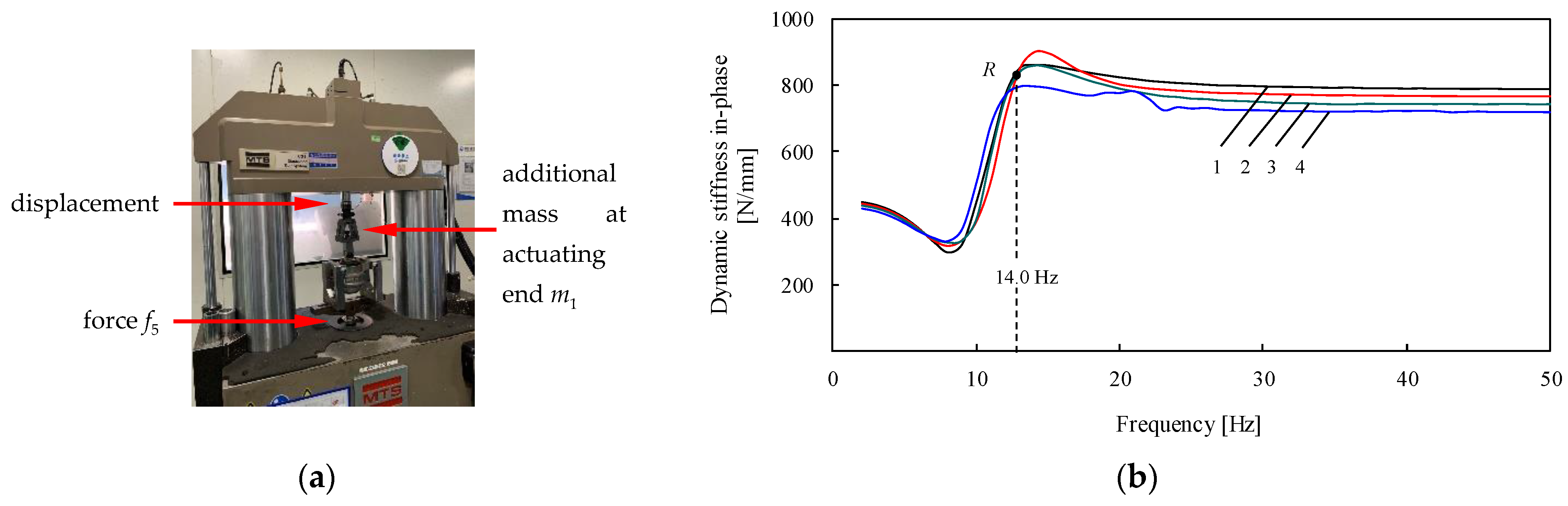
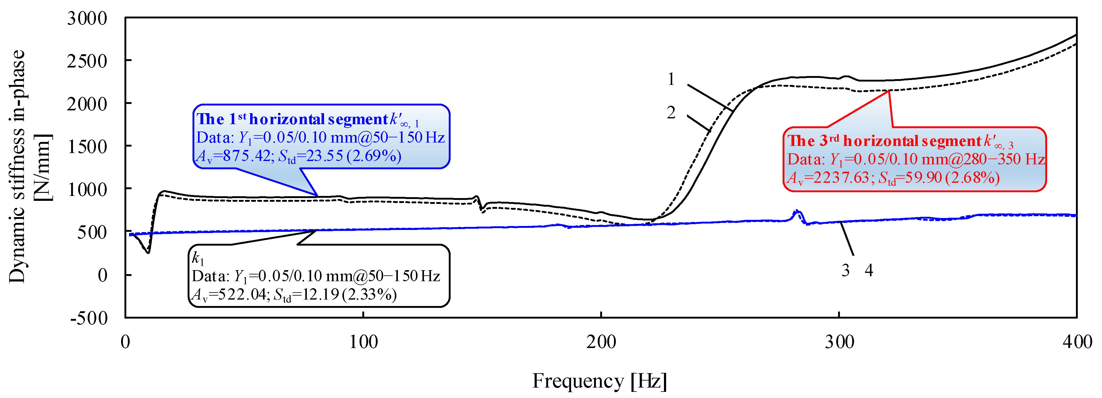
5.1. Passive Dynamics Test and Parameters Identification

As shown in Table 1, the input of the passive dynamics is the engine-side displacement Y₁, and the output is the engine-side force F₁ and chassis-side force F₅. The distinct features were the fixed point and the 1st, 2nd and 3rd horizontal segments according to the theoretical results. The experiment was designed and performed based on the MTS elastomer test system. It should be noted that the drive-point dynamics test was not supported and could not be measured. Therefore, the distinct features of the 2nd horizontal segment test results are not discussed.

The experimental setup and passive dynamics of cross-point dynamics are shown in Figure 4. The specific fixtures shown in Figure 4a were needed for the tests; thus, the dynamics tested contained the modal of fixtures in the high-frequency band. Figure 4b shows the features of the amplitude dependence, and the fixed-point R in the dynamic stiffness in-phase agrees well with the analysis.

The cross-point passive dynamics in the mid-and high-frequency bands were measured at 2–400 Hz, as shown in Figure 5. The figure shows the 1st horizontal segment $k_{\infty ,1}^{\prime }$ and the 3rd horizontal segment $k_{\infty ,3}^{\prime }$. However, the 3rd horizontal segment was distorted by the fixture modalities; therefore, it was marked by a red text box as a warning. It is difficult to obtain accurate and reliable cross-point dynamics in higher frequency bands because the test generally requires a complex and bulky fixture system, as shown in Figure 4a.

Therefore, the bulk stiffness K_u1 of the upper fluid chamber and the equivalent piston area A₁ of the main rubber spring, can be identified based on the fixed point R and the 1st horizontal segment $k_{\infty ,1}^{\prime }$ by passive dynamics in the mid- and low-frequency bands according to Equation (11). The identification procedure and results are shown in entries 2.1–2.7 of the Table A1.

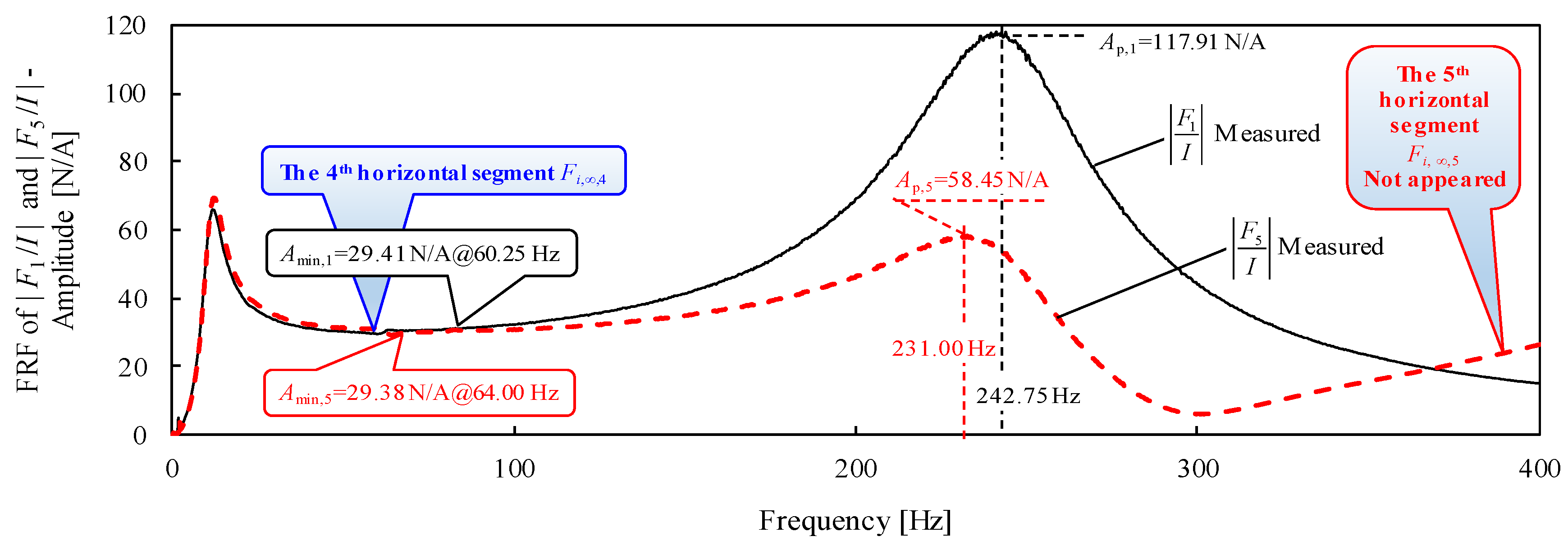
5.2. Active Dynamics Test in Fluid-Filled State and Parameters Identification

As shown in Table 1, the input of the active dynamics in the fluid-filled state is the actuator current I, and the outputs are the engine-side force F₁ and chassis-side force F₅. The frequency and amplitude of the resonance peak, the 4th horizontal segment and the 5th horizontal segment can be obtained. In contrast to the passive dynamics test, the active dynamics test does not need to be excited and measured by the MTS elastomer test system. The tests were performed and measured by Siemens Simcenter Testlab with the corresponding equipment. The active mount was assembled on the MTS test system, which maintains the boundary conditions consistent with the passive dynamics test.

Moreover, improvements in the modalities of fixtures were achieved through structure optimization and material selection. The effective bandwidth of the FRFs on the upper side reached 400 Hz. Even in the non-fluid state, the effective bandwidth of the FRFs on the upper side reached 1000 Hz. The active dynamics in the filled fluid are shown in Figure 6, and it is clear that there is a 4th horizontal segment before the mover resonance peak. Unfortunately, the 5th horizontal segment did not appear owing to the distortion by the fixture modality on the lower side, which is also indicated by a red text box as a warning.

The distinct features, f_p,1 and A_p,1, can be obtained from the test results. The 4th horizontal segment F_i,∞,4 is slightly concave and is induced by the mover modal. The lowest point is closest to the 4th horizontal segment; therefore, the minimum value A_min was chosen as the estimate of F_i,∞,4. Thus, coupling parameter A₃K₃ can be identified by F_i,∞,4 according to Equation (19). Subsequently, ξ₃ and f_n3 can be identified by F_i,∞,4 and A_p,1 successively according to Equation (21). The detailed procedure and results are presented in 3.1–3.6 of the Table A1.

The natural frequency of the actuator mover in the fluid-filled state is f_n3 = 246.68 Hz, which is higher than that of the fluid channel (f_n2 = 14.00 Hz) identified by passive dynamics. Therefore, it is reasonable to divide the frequency into three frequency bands, based on these two natural frequencies. The mover resonance band of the FRF |F₅/I| is easily affected by the modals of the fixture at the lower side. Therefore, it is not recommended to use the tested |F₅/I| for parameter identification in the high-frequency band.

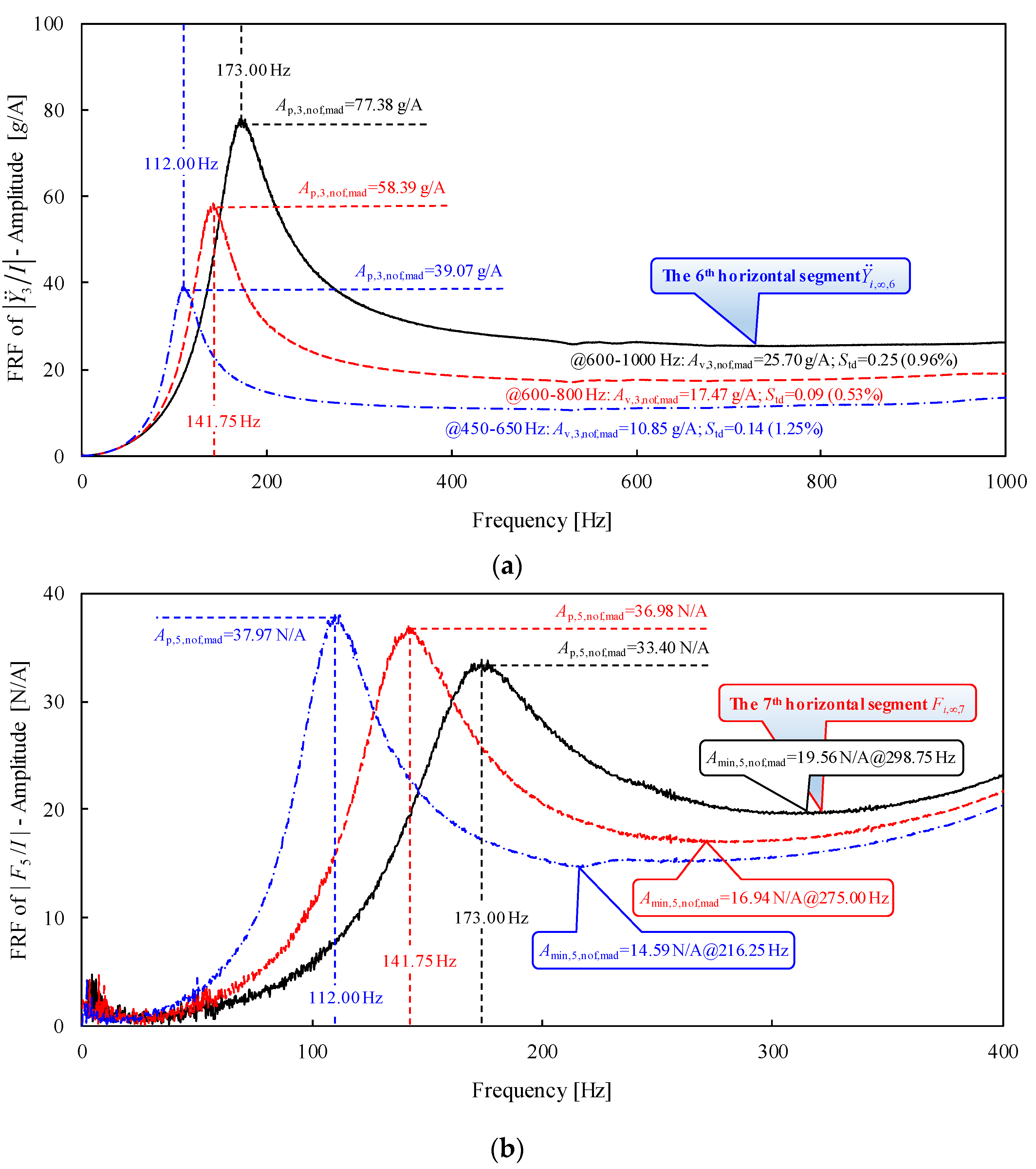
5.3. Active Dynamics Test in Non-Fluid State and Parameters Identification

As shown in Table 1, the input of the active dynamics in the non-fluid state is the actuator current I, and the outputs are the mover acceleration ${\ddot{Y}}_3$ and chassis-side force F₅. Distinct features such as the frequency and amplitude of the resonance peak, the 6th horizontal segment and the 7th horizontal segment can be obtained. The test was designed to decouple parameters K_u1 and A₃K₃, and the test equipment was the same as that used in Section 5.2.

The tests were performed under boundary conditions with the main rubber spring removed. For the measurement of the mover acceleration ${\ddot{Y}}_3$, the accelerometer was attached to the mover; thus, its mass effect had to be considered for the identification of key parameters. Accordingly, tests with three different added masses were performed to verify the consistency and stability of the mass identification results. The result for the actuator mover mass identified directly was the parameter with added mass, defined as m_3,nof,mad. Subsequently, the parameter m_3,nof can be calculated by subtracting the added mass.

The FRF curves measured with three different added masses are shown in Figure 7. The added masses were 8.90 g, 38.97 g and 93.03 g. Figure 7a,b shows the FRFs of $\left|{\ddot{Y}}_3/I\right|$ and |F₅/I|, which clearly show the mover resonance peaks, 6th horizontal segment ${\ddot{Y}}_{i,\infty ,6}$, and 7th horizontal segment F_i,∞,7. This indicates that the two FRFs for the same added mass have the same peak frequency f_p,3,nof,mad, which is consistent with the analysis using Equation (25). For the distinct features of the 6th horizontal segment shown in Figure 7a, the mover acceleration FRFs converged to a different horizontal segment influenced by different added masses according to Equation (23). For the distinct features of the 7th horizontal segment shown in Figure 7b, the test results of the chassis-side force FRFs changed with the added mass, which should theoretically converge to the same horizontal segment k_M, according to Equation (25). The FRFs increased owing to the influence of the fixture modalities at 550 Hz on the lower side.

As the added mass increased, the 7th horizontal segment decreased and gradually approached parameter k_M. When the added mass m_ad = 93.03 g, the minimum value in the concave section was A_{min,5,nof,mad} = 14.59 N⋅A⁻¹, which was already very close to the true value of k_M = 14 N⋅A⁻¹.

Based on the distinct features of $\left|{\ddot{Y}}_3/I\right|$, which are more suitable for identification than |F₅/I|, the parameter m_3,nof,mad can be obtained, which can then be used to identify the linear stiffness k₃ and viscous damping c_3,nof of the decoupler membrane. Subsequently, the net mover mass m_3,nof can be obtained by subtracting the added mass, so that the natural frequency f_n3,nof and the damping ratio ξ_3,nof of the mover system can be obtained. The detailed procedure is listed in 4.1–4.12 of the Table A1.

Based on all parameters identified by distinct features, the following key parameters can be identified: the equivalent piston area A₃ and bulk stiffness K₃ of the decoupler membrane_; bulk stiffness K₁ of the main rubber spring_; total mass m₃ of the mover including the attached fluid in the fluid-filled state; and total viscous damping c₃. These parameters are listed in 5.1–5.5 of the Table A1.

Considering the limitations of the test equipment and low fixture modalities, the resonance of the fluid channel and actuator mover, and the 1st, 4th and 6th horizontal segment can be applied to identify all the key parameters of the AHM-IT-DM-OCA.

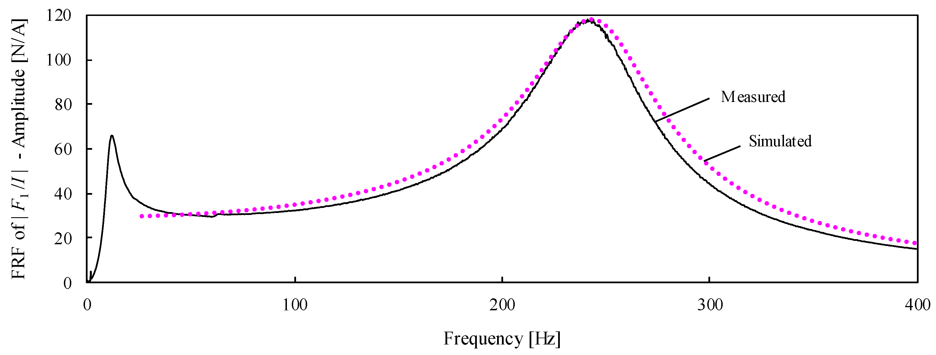
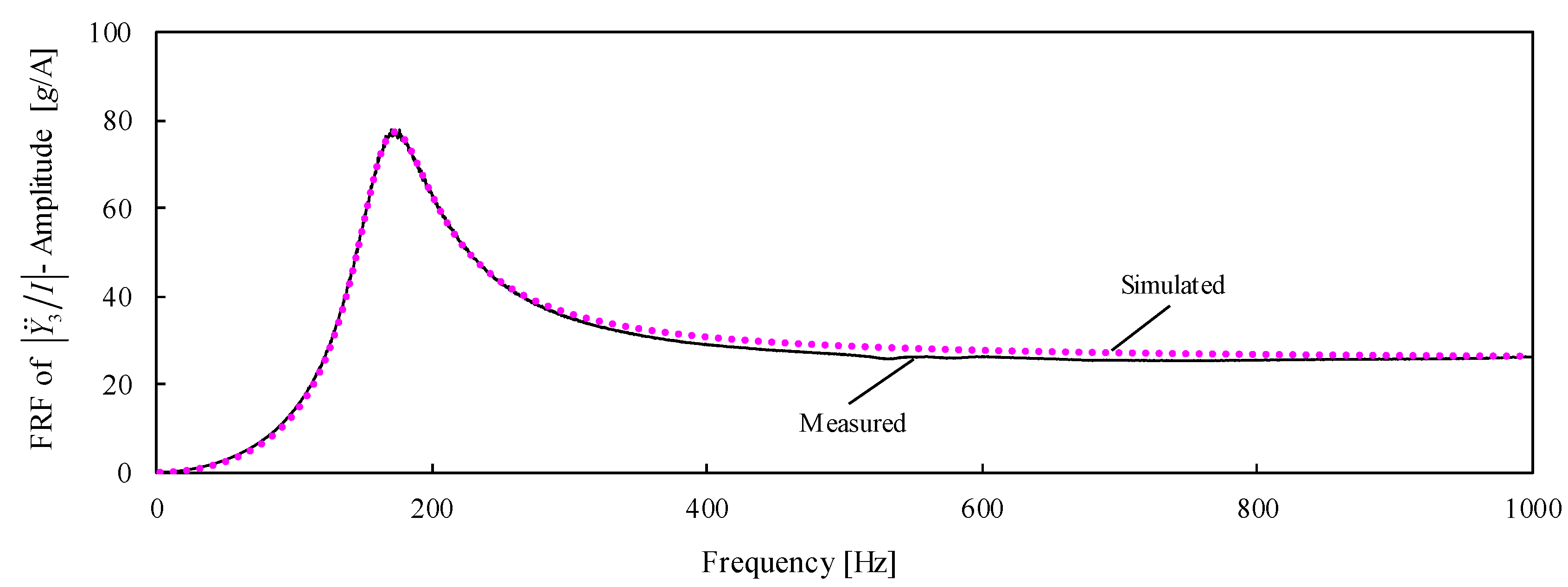
5.4. Simulation of Active Dynamics Based on the Identified Parameters

Since the tests were performed under three different added masses, three sets of key parameters were identified by the test results. The results are compared in

Table 2. Consistency check of identified parameters for an AHM-IT-DM-OCA.

4.1. Added Mass, mad (g)	mad,1	mad,2	mad,3	Consistency of Obtained Results
	8.90	38.97	93.03	Mean	Standard Deviation	Relative Std
* 4.8. Linear stiffness of the decoupler membrane, k3 (N⋅mm−1) (independent of added mass)	61.95	61.91	62.62	62.16	0.40	0.64%
* 5.1. Equivalent piston area of the decoupler membrane, A3 (mm2)	1320.03	1319.21	1334.48	1324.57	8.61	0.65%
* 5.2. Dynamic bulk stiffness of the decoupler membrane, K3 (GN⋅m−5)	35.55	35.57	35.17	35.43	0.23	0.64%
* 5.3. Dynamic bulk stiffness of the main rubber spring, K1 (GN⋅m−5)	121.53	121.27	126.25	123.02	2.80	2.28%
* 5.4. Total mover mass including attached fluid in the fluid-filled state, m3 (g)	113.93	113.62	119.66	115.74	3.40	2.94%
* 5.5. Total viscous damping of the mover system in the fluid-filled state, including damping of the fluid and damping of the decoupler membrane, c3 (N⋅s⋅m−1)	44.40	44.28	46.63	45.10	1.32	2.93%

. The key parameters identified by the different added-mass tests showed good consistency, and the maximum relative standard deviation was only 2.94%.

Moreover, the physical rationality of the key parameter results shown in the Table A1 should be noted. The results identified in the fluid-filled state were much higher than those in the non-fluid state, such as the mover mass (m₃ >> m_3,nof) and viscous damping of the mover (c₃ >> c_3,nof)

A series of numerical simulations were carried out based on the mathematical models in the mid- and high-frequency bands using the parameters in the third column in the Table A1 to verify the correctness of the key parameters. The simulation results were compared with the experimental dynamics results, as shown in Figure 8 and Figure 9. For the curves related to force f₁ and acceleration ${\ddot{y}}_3$, the simulations agreed well with the experiments in the mid- and high-frequency bands.

6. Conclusions

(1)

Distinct features of the dynamics and key parameter identification were systematically investigated based on a nonlinear lumped parameter model of the AHM-IT-DM-OCA. A method for simplifying the mathematical model is proposed in the low-, mid-, and high-frequency bands, which are divided into two resonance frequencies of the fluid channel and actuator mover. The simplified model in the mid- and high-frequency bands is linear, which is attributed to the negligible nonlinear factors of the fluid channel and the linear output of the actuator.

(2)

The distinct features of the dynamics, which include three resonances and seven horizontal segments, are revealed. Experimental validations based on a series of tests have shown only three resonances of the fluid channel and actuator mover, and the 1st, 4th, and 6th horizontal segments can be applied to identify all key parameters owing to the limitations of the test equipment and low fixture modalities.

(3)

The distinct features of passive and active dynamics in fluid-filled and non-fluid states should be analyzed successively rather than independently. Passive dynamics are the foundation that provide a method for model simplification and basic parameters. The active dynamics in the non-fluid state are extensions of the identification of all key parameters, which decouples the complex items composed of multiple key parameters. A complete procedure for the identification of all six key parameters is established based on the distinct features of the dynamics. This is compared with previous study’s identification of only two parameters based on the fixed point of passive dynamics.

(4)

The consistency of the key parameters identified by the procedure is presented based on experiments with different added masses. The physical rationality is presented by comparing the results under fluid-filled and non-fluid states. The correctness is demonstrated by the agreement between the simulated active dynamics and the experimental ones. All key parameters identified by this systematic method are sufficiently accurate to be applied for future research on algorithms and the performance of active control.

References

1. Chakrabarti, S.; Dapino, M.J. Design and modeling of a hydraulically amplified magnetostrictive actuator for automotive engine mounts. In Proceedings of the SPIE 7645, the Industrial and Commercial Applications of Smart Structures Technologies, San Diego, CA, USA, 29 March 2010. [Google Scholar] [CrossRef]
2. Kraus, R.; Millitzer, J.; Hansmann, J.; Wolter, S.; Jackel, M. Experimental study on active noise and active vibration control for a passenger car using novel piezoelectric engine mounts and electro dynamic inertial mass actuators. In Proceedings of the ICAST 2014—25th International Conference on Adaptive Structures and Technologies, The Hague, The Netherlands, 6 October 2014. [Google Scholar]
3. Foumani, M.S.; Khajepour, A.; Durali, M. Application of Shape Memory Alloys to a New Adaptive Hydraulic Mount. In Proceedings of the International Body Engineering Conference & Exhibition and Automotive & Transportation Technology Congress, Paris, France, 9–11 July 2002. [Google Scholar] [CrossRef]
4. Hausberg, F.; Scheiblegger, C.; Pfeffer, P.; Plöchl, M.; Hecker, S.; Rupp, M. Experimental and analytical study of secondary path variations in active engine mounts. J. Sound Vib. 2015, 340, 22–38. [Google Scholar] [CrossRef]
5. Hausberg, F.; Plöchl, M.; Rupp, M.; Pfeffer, P.; Hecker, S. Combination of map-based and adaptive feedforward control algorithms for active engine mounts. J. Vib. Control 2017, 23, 3092–3107. [Google Scholar] [CrossRef]
6. Christopherson, J.; Jazar, G.N. Dynamic behavior comparison of passive hydraulic engine mounts. Part 2: Finite element analysis. J. Sound Vib. 2006, 290, 1071–1090. [Google Scholar] [CrossRef]
7. Zhou, D.; Zuo, S.; Wu, X. A Lumped Parameter Model Concerning the Amplitude-Dependent Characteristics for the Hydraulic Engine Mount with a Suspended Decoupler. SAE Tech. Pap. 2019, 1, 936. [Google Scholar] [CrossRef]
8. Wang, L.-R.; Wang, J.-C.; Hagiwara, I. An integrated characteristic simulation method for hydraulically damped rubber mount of vehicle engine. J. Sound Vib. 2005, 286, 673–696. [Google Scholar] [CrossRef]
9. Wang, L.-R.; Wang, J.-C.; Lu, Z.-H.; Hagiwara, I. Finite element-based parameter estimations for a characteristic simulation model of a hydraulically damped rubber mount for vehicle engines. Proc. Inst. Mech. Eng. Part D J. Automob. Eng. 2007, 221, 1273–1286. [Google Scholar] [CrossRef]
10. Shi, W.-K.; Mao, Y.; Jiang, X.; Chen, Z.-Y.; Pan, B. Parameter identification and dynamic characteristics of semi-active hydraulic mount. J. Jilin Univ. 2014, 44, 605–611. [Google Scholar] [CrossRef]
11. Zhang, Y.; Zhang, J.; Shangguan, W.-B. Modeling and experimental study of a passive hydraulic engine mount with inertia and direct-Decoupler. Chin. J. Mech. Eng. 2008, 21, 31–35. [Google Scholar] [CrossRef]
12. Guo, R.; Wei, X.-K.; Zhou, S.-Q.; Gao, J. Parametric identification study of an active engine mount: Combination of finite element analysis and experiment. Proc. Inst. Mech. Eng. Part D J. Automob. Eng. 2019, 233, 427–439. [Google Scholar] [CrossRef]
13. Kyprianou, A.; Giacomin, J.; Worden, K.; Heidrich, M.; Bocking, J. Differential evolution based identification of automotive hydraulic engine mount model parameters. Proc. Inst. Mech. Eng. Part D J. Automob. Eng. 2000, 214, 249–264. [Google Scholar] [CrossRef]
14. Zheng, L.; Liu, Q.-B.; You, Z.-L.; Pang, J.; Xu, X.-M.; Chen, D.-J. Development of Modified Lumped Parameter Model involving Amplitude-dependence Characteristics on Semi-active Engine Mount and Experimental Verification. Chin. J. Mech. Eng. 2017, 53, 98–105. [Google Scholar] [CrossRef]
15. Chen, S.-W.; Li, R.; Du, P.-F.; Zheng, H.-W.; Li, D.-Y. Parametric Modeling of a Magnetorheological Engine Mount Based on a Modified Polynomial Bingham Model. Front. Mater. 2019, 6, 68. [Google Scholar] [CrossRef]
16. He, S.; Rajendra, R. Estimation of amplitude and frequency dependent parameters of hydraulic engine mount given limited dynamic stiffness measurements. Noise Control Eng. J. 2005, 53, 271–285. [Google Scholar] [CrossRef]
17. Li, L. Study of the Lumped Parameter Models and Parameters Identification of Hydraulic Bushing. Appl. Mech. Mater. 2013, 321, 1805–1811. [Google Scholar] [CrossRef]
18. Manikantan, R.; Chakraborty, S.; Uchida, T.K.; Vyasarayani, C.P. Parameter Identification in Nonlinear Mechanical Systems with Noisy Partial State Measurement Using PID-Controller Penalty Functions. Mathematics 2020, 8, 1084. [Google Scholar] [CrossRef]
19. Chai, T.; Dreyer, J.T.; Singh, R. Time domain responses of hydraulic bushing with two flow passages. J. Sound Vib. 2014, 333, 693–710. [Google Scholar] [CrossRef]
20. Chai, T.; Dreyer, J.T.; Singh, R. Frequency domain properties of hydraulic bushing with long and short passages: System identification using theory and experiment. Mech. Syst. Signal Process. 2015, 56, 92–108. [Google Scholar] [CrossRef]
21. Yang, C.-F.; Yin, Z.-H.; Shangguan, W.-B.; Duan, X.-C. A Study on the Dynamic Performance for Hydraulically Damped Rubber Bushings with Multiple Inertia Tracks and Orifices: Parameter Identification and Modeling. Shock Vib. 2016, 2016, 3695950. [Google Scholar] [CrossRef] [Green Version]
22. Fan, R.-L.; Dou, Y.-F.; Ma, F.-L. Fixed Points on Active and Passive Dynamics of Active Hydraulic Mounts with Oscillating Coil Actuator. Actuators 2021, 10, 225. [Google Scholar] [CrossRef]
23. Fan, R.-L.; Fei, Z.-N.; Zhou, B.-Y.; Gong, H.-B.; Song, P.-J. Two-step dynamics of a semiactive hydraulic engine mount with four-chamber and three-fluid-channel. J. Sound Vib. 2020, 480, 115403. [Google Scholar] [CrossRef]
24. Gao, Z.-Q.; Wang, B.-R. Fluid Mechanics; Science Press: Beijing, China, 2017. [Google Scholar]
25. Fan, R.-L.; Lu, Z.-H. Fixed points on the nonlinear dynamic properties of hydraulic engine mounts and parameter identification method: Experiment and theory. J. Sound Vib. 2007, 305, 703–727. [Google Scholar] [CrossRef]
26. Zhang, Y.-M. Mechanical Vibrations; Tsinghua University Press: Beijing, China, 2019. [Google Scholar]
27. Li, Y.; Jiang, J.-Z.; Neild, S.A. Optimal fluid passageway design methodology for hydraulic engine mounts considering both low and high frequency performances. J. Vib. Control 2019, 25, 2749–2757. [Google Scholar] [CrossRef]
Figure 1. Configuration schematics for the AHM-IT-DM-OCA [22]: 1. rubber bellow; 2. lower chamber; 3. inertia track; 4. decoupler membrane; 5. upper chamber; 6. main rubber spring; 7. actuator mover; 8. coil; 9. permanent magnet.
Applsci 12 08547 g001
Figure 2. Lumped parameter mechanical model for the AHM-IT-DM-OCA [22].
Applsci 12 08547 g002
Figure 3. Low-, mid-, and high-frequency bands for the dynamic analysis of AHM-IT-DM-OCA [22].
Applsci 12 08547 g003
Figure 4. Experimental validation of passive dynamics in mid- and low-frequency bands. (a) experimental setup, (b) dynamic stiffness in-phase. Key: the numbers 1–4 correspond to the excitation amplitudes of Y1 = 0.4 mm, 0.6 mm, 0.8 mm, and 1.0 mm, respectively; R is the fixed point in dynamic stiffness in-phase.
Applsci 12 08547 g004
Figure 5. Experimental validation of passive dynamics in mid- and high-frequency bands. Dynamic stiffness in-phase and the 1st and 3rd horizontal segments; Key: numbers 1 and 2 correspond to the excitation amplitudes of Y1 = 0.05 mm and 0.10 mm; numbers 3 and 4 correspond to Y1 = 0.05 mm and 0.10 mm for the main rubber spring of the AHM-IT-DM-OCA.
Applsci 12 08547 g005
Figure 6. Experimental validation of active FRFs in the fluid-filled state. Key: Measured FRF |F1/I| (—); measured FRF |F5/I| (- -).
Applsci 12 08547 g006
Figure 7. Experimental validation of active FRFs in the non-fluid state. (a) FRF of | Y ¨ 3 / I | (0–1000 Hz), (b) FRF of |F5/I| (0–400 Hz). Key: Added masses mad = 8.90 g (––); mad = 38.97 g (– –); mad = 93.03 g ().
Applsci 12 08547 g007
Figure 8. Simulation validation of the active FRF of |F1/I| at 25–400 Hz for the fluid-filled state. Key: Measured (–––); Simulated (·····).
Applsci 12 08547 g008
Figure 9. Simulation validation of the active FRF of | Y ¨ 3 / I | at 0–1000 Hz for the non-fluid state. Key: Added masses mad = 8.90 g; Measured (–––); Simulated (·····).
Applsci 12 08547 g009