Article

Safe, Smooth, and Fair Rule-Based Cooperative Lane Change Control for Sudden Obstacle Avoidance on a Multi-Lane Road †

1
Graduate School of Integrated Science and Technology, Shizuoka University, Hamamatsu 432-8011, Japan
2
College of Engineering, Academic Institute, Shizuoka University, Hamamatsu 432-8011, Japan
3
Graduate School of Science and Technology, Shizuoka Univeristy, Hamamatsu 432-8011, Japan
*
Author to whom correspondence should be addressed.
This paper is an extended version of our paper published in VTC2022-Spring.
Appl. Sci. 2022, 12(17), 8528; https://doi.org/10.3390/app12178528
Submission received: 29 July 2022 / Revised: 20 August 2022 / Accepted: 22 August 2022 / Published: 26 August 2022
(This article belongs to the Special Issue Data Dissemination in Vehicular Networks)

Abstract

:
When an unexpected obstacle occupies some of the lanes on a multi-lane highway, connected vehicles (CVs) may be able to avoid it cooperatively. For example, a CV that detects the obstacle first can immediately notify the following vehicles of the obstacle by using vehicle-to-vehicle (V2V) communication. In turn, the following vehicles can take action to avoid the obstacle smoothly using wide range behind the obstacle without sacrificing safety and ride comfort. In this study, we propose a method to realize safe, smooth, and fair wide-range cooperative lane changing, reacting to a sudden obstacle on the road. The proposed method is based on the authors’ previous work, which utilizes multi-hop communication to share the obstacle position and controls the inter-vehicular distance of vehicles away from the obstacle to assist in a smooth lane changing operation, while existing lane-changing methods for CVs focus on microscopic operation around the obstacle. Though the previous work treats only a two-lane road, the proposed method is extended to work on a three- or more lane road assuming only one lane is blocked. In the proposed scheme, each vehicle approaching the obstacle selects a lane to change to in accordance with the obstacle’s location and the vehicle density in each lane estimated from the beacon messages broadcast by each CV, thereby improving traffic fairness among all lanes without degrading safety or ride comfort. We confirmed the effectiveness of the proposed scheme on realizing fairness among lanes, safety, ride comfort, and traffic throughput through comprehensive simulations of a two-lane road and a three-lane road with various traffic scenarios.

1. Introduction

In recent years, safe driving support and automated driving technology using vehicle-to-vehicle (V2V) communication have been actively studied. The methods used in these studies are expected to improve the safety and efficiency of traffic flow because vehicles can cooperate by sharing their position, speed, and other driving information with surrounding vehicles [1]. If an obstacle (e.g., a disabled vehicle or spilled cargo) suddenly blocks part of a multilane road, a traffic jam may occur because of the decrease in the road capacity [2]. Even if the road capacity after the blockage is larger than the offered road traffic, traffic jams may occur because vehicles in the blocked lane need to move to the neighboring lane, which leads to the sudden deceleration of vehicles [3] as shown in Figure 1a. In this situation, if the vehicle that detected the obstacle immediately notifies the following vehicles of the obstacle’s position by using V2V communication, the following vehicles will be able to take action to avoid the obstacle in advance, thereby preventing a traffic jam, as shown in Figure 1b.
Currently, the existence of an obstacle on the road is notified to drivers via the internet (e.g., Google Maps [4] and Waze [5]), broadcast system (e.g., VICS—vehicle information and communication system [6]), and roadside digital signboards. If someone, e.g., general drivers or a road operator, finds an obstacle on the road, the control center is notified of the information. Then the information is presented to drivers via car navigation systems, smartphone apps, and roadside signboards. Since there is a non-negligible delay between the detection of the obstacle and the time that the information reaches vehicles approaching the obstacle, drivers and autonomous vehicles moving near the obstacle cannot react to the obstacle quickly. Even if the existence of an obstacle is notified to drivers/autonomous vehicles, they do not know the best operation, e.g., acceleration or which lane to change to, to avoid the obstacle, not leading to traffic jams. On the other hand, the proposed method enables the vehicles moving in a wide range behind the obstacle to know the existence of the obstacle and how to react to it properly (e.g., making space to accommodate lane-changing vehicles and selecting a lane), not leading to traffic jams and uncomfortable driving maneuvers. Since the notification is sent to vehicles in a wide range, even human drivers can react to it with time to spare.
Our previous work [7] proposed a simple rule-based lane change control strategy for the smooth avoidance of a suddenly appearing road obstacle by using V2V communication. In this strategy, the vehicle that detects an obstacle uses multi-hop communication to share the obstacle’s position with the vehicles behind it. Vehicles behind the obstacle that receive the message decrease their speed to double the normal time headway so that vehicles in the blocked lane can change lanes smoothly and safely, as shown in Figure 2. In the simulations of a two-lane road using the traffic flow simulator, simulation of urban mobility (SUMO) [8], this scheme improves traffic throughput and fairness among lanes compared with the scheme using only non-connected vehicles (NCVs).
However, this strategy only considered a two-lane road. This paper extends this strategy to work when one lane is obstructed on a three- or more lane road. When the three-lane road’s rightmost (edge) lane is obstructed, if only vehicles in the rightmost lane change lanes, traffic will concentrate in the center lane. In contrast, vehicles in the leftmost (edge) lane will move smoothly without interference from increased traffic from other lanes. In this case, only vehicles initially traveling in the right and center lanes will experience delays in overtaking the obstacle. As the result, traffic distribution among lanes will be unfair. Therefore, the proposed extended strategy aims to control lane changes of vehicles in all lanes to achieve traffic fairness among all lanes without sacrificing safety or ride comfort. In this strategy, each vehicle approaching the obstacle selects a suitable lane in accordance with the obstacle’s location and the vehicle density in each lane estimated from the beacon messages broadcast by each CV.
The main contributions of this paper are listed below:
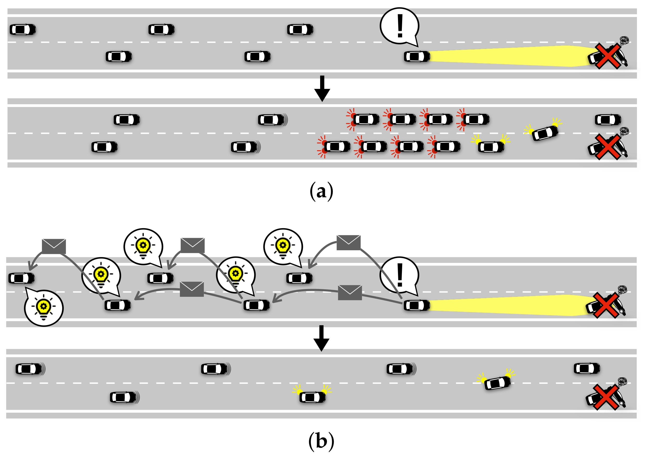
  • We propose a method to realize safe, smooth, and fair wide-range cooperative lane changing, reacting to a suddenly appearing obstacle on the road. In this strategy, a CV that detects the obstacle immediately notifies the following vehicles of the obstacle by using V2V communication. In turn, the following vehicles can take action to avoid the obstacle smoothly using a wide range behind the obstacle without sacrificing safety and ride comfort. To the authors’ knowledge, existing studies focus on microscopic control around obstacles and do not discuss the control of traffic in a wide range, a few kilometers, as addressed in this study. The microscopic operation for lane-changing trajectory planning is out of this paper’s scope.
  • The proposed method works when one lane is obstructed on a three- or more lane road. On three- or more lane roads, vehicles can have multiple choices to change lanes. Thus, we develop a method to select a suitable lane that will not cause unfairness among lanes and deteriorate ride comfort.
  • We confirm the effectiveness of the proposed method in realizing fairness among lanes, safety, ride comfort, and traffic throughput through simulations of a two-lane road and a three-lane road with various traffic scenarios, assuming that the vehicles’ microscopic operation depends on the lane change model of SUMO.
This paper is an extended version of a conference paper presented at VTC2022-Spring [9]. The main differences between this paper and the conference paper are in the simulation model, performance metrics, and results. The details are as follows.
  • The road length in the simulation environment is increased from 1   km to 2   km in order to provide sufficient free space before vehicles encounter an obstacle.
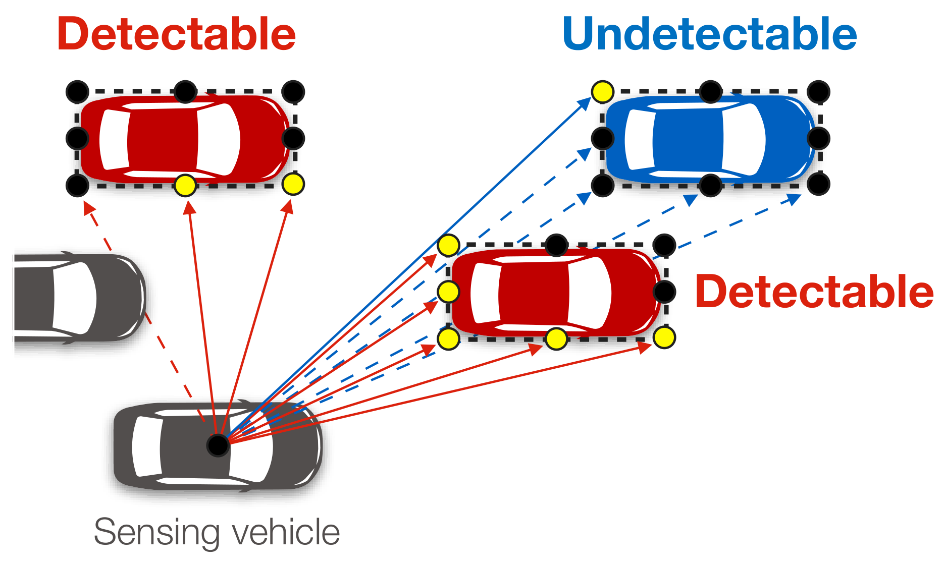
  • The simulations consider occlusion in a vehicle detection model.
  • Two vehicle behavior models (Proposed_NoPrelim and Proposed_NoAdaptive) are introduced to confirm the effectiveness of the proposed scheme.
  • A fairness equation is introduced to quantitatively evaluate the fairness level in the simulation evaluation.
  • A safety metric is introduced in the simulation evaluation.
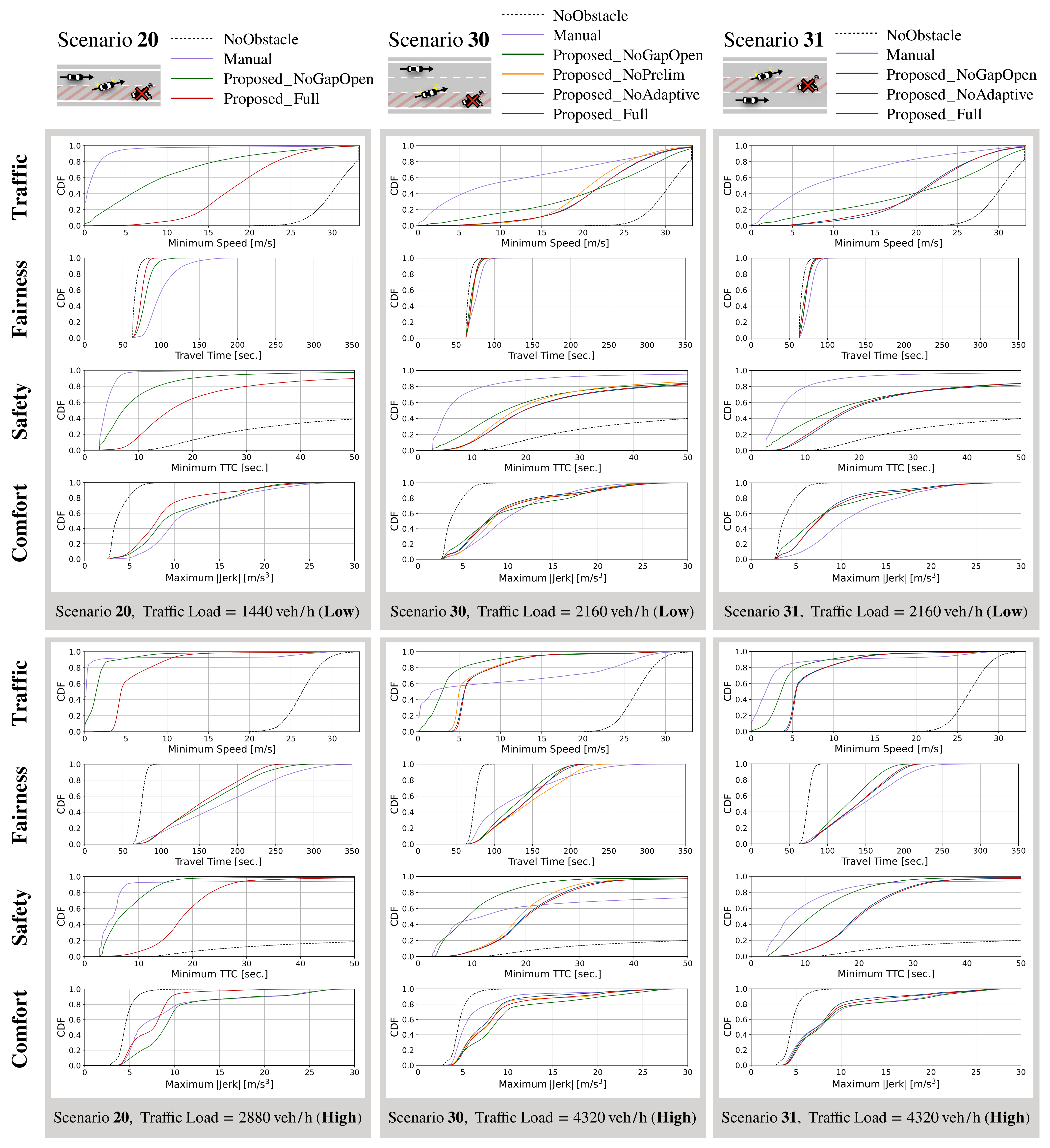
  • Cumulative distribution function (CDF) graphs are created for each performance metric to analyze the simulation results in more detail.
  • Simulations are conducted with various traffic loads to evaluate the performance of the proposed method comprehensively and with various zone sizes of the proposed scheme to investigate the impact of the zone sizes.
The remainder of the paper is structured as follows. Section 2 summarizes the related work. Section 3 describes the proposed scheme, Section 4 explains the simulation model, and Section 5 presents the simulation results and a discussion from the viewpoints of traffic throughput, fairness, safety, and ride comfort. Section 6 concludes the paper with suggestions for future work.

2. Related Work

Lane changing is one of the common and essential operations of vehicles and has a significant influence on traffic safety and efficiency [10]. With the rapid development of V2V communications, most vehicles will have the ability to exchange information with each other and perform cooperative lane changes, improving the efficiency and safety of the entire traffic. Automated lane changing by connected and autonomous vehicles (CAVs) has been studied actively. Wang et al. propose a cooperative lane change strategy based on model predictive control (MPC), which realizes a safe and effective lane change through the cooperation between a lane-changing vehicle and vehicles on the target lane [11]. Their simulation results show that the deceleration of the follower vehicles can be mitigated. Further, the shock wave propagated in traffic flow can be alleviated compared with a traditional lane change. Luo et al. propose a multi-vehicle cooperative automated lane-change maneuver for scenarios with three lanes and two lane-change vehicles [12]. They classify cooperative automated multi-lane-change scenarios into two types: same-direction lane change and intersectant-direction lane change, which facilitates the construction of a mathematical model. Lane-change vehicles determine the lane-change type based on information from all vehicles involved and plan safe trajectories. Li et al. propose a dynamic cooperative trajectory planning model for lane changes of autonomous driving on the traffic scene with multiple mandatory lane change demands [13]. This model divides the traffic flow into groups, which simplifies the problem. Vehicles in the same group cooperatively plan their trajectory so that they can drive safely with each other. These above-mentioned research works mainly focus on the trajectory planning of lane change in a limited area; that is, a few vehicles that want to change lanes and their neighboring vehicles are considered. Lane change maneuvers discussed in the literature are obtained mainly by solving an optimization model, such as MPC.
Since merging from an on-ramp lane to the highway is one of the most challenging driving scenarios, there has been much research on cooperative lane change for on-ramp flows. In the merging scenario, vehicles in the lane that vanishes (i.e., an on-ramp lane or a merging lane) are forced to change lanes, and they know the position of the merging point beforehand. The Car 2 Car Communication Consortium (C2C-CC) [14] aims to improve safety in merging support control by recognizing the existence of NCVs by using collective perception [15]. The Federal Highway Administration [16] developed the Cooperative Automation Research Mobility Application (CARMA) as an open-source software platform to promote the verification and evaluation of automated cooperative driving technologies. In the merging support of CARMA, the mainline vehicle and the on-ramp vehicle exchange information (e.g., position and speed) by using vehicle-to-infrastructure (V2I) and V2V communication and control their speed for smooth merging [17]. Ding et al. propose a rule-based adjusting algorithm to achieve a near-optimal merging sequence for on-ramp vehicles and mainline vehicles [18]. Jing et al. propose a cooperative multiplayer game-based optimization framework to provide optimal trajectories for the CAVs in a merging zone [19]. These studies assume that all vehicles are CAVs and focus on microscopic operations, i.e., they treat the mobility of vehicles in a narrow area.
Drivers and autonomous vehicles cannot know the existence of a sudden obstacle on the road beforehand. Thus, avoiding such an obstacle by lane changing is more difficult than lane changing at a fixed merge point. The Multi-Car Collision Avoidance (MuCCA) project has been developing a next-generation driver aid system that uses V2V communication to avoid multi-car collisions on highways [20]. Wartnaby et al. proposed a scheme for optimizing the trajectories of MuCCA-equipped vehicles (MEV) when they avoid an obstacle [21]. In this scheme, MEVs compute two trajectories: a “desired” trajectory, based on only the predicted trajectories of the surrounding non-MEVs, and a “planned” trajectory, based on the planned trajectories of the surrounding MEVs and the predicted trajectories of the surrounding non-MEVs. Each MEV broadcasts two trajectories and attempts to (weakly) avoid the desired trajectories of the other MEVs. Bae et al. propose a control framework for autonomous lane changing due to merged lanes or an obstacle on the road in highly dense traffic on the highway [22]. The control framework incorporates a recurrent neural network (RNN) architecture, namely a state-of-the-art social generative adversarial network (SGAN), to predict the interactive motions of multiple drivers. They focus on heavy traffic scenarios where vehicles cannot merge into a lane without cooperating with other drivers. These studies focus on microscopic operation. On the other hand, our work focuses on the macroscopic operation of vehicles. We focus on cooperative lane change over a wide range behind an obstacle aiming to avoid heavy traffic jams, improve the total traffic, improve the fairness of traffic between lanes, and avoid the degradation of passengers’ comfort.

3. Proposed Scheme

This section describes our lane-change control scheme for avoiding a suddenly appearing obstacle on roads with three or more lanes while preventing any deterioration in safety, ride comfort, and traffic fairness among lanes. In this scheme, vehicles avoid the obstacle by following simple rules after being notified of the obstacle’s existence through V2V communication. In addition, each vehicle approaching the obstacle selects a lane to which will move in accordance with the obstacle’s location and the vehicle density in each lane estimated from the beacon messages broadcast by each connected vehicle (CV), thereby improving the fairness of the traffic distribution among lanes.

3.1. Assumed Environment

We assume the following environment.
  • Vehicles are equipped with sensors such as cameras and LiDAR, which can detect vehicles, road structures, and obstacles.
  • Vehicles are equipped with a V2V communication function and are operated by an automatic driving system or a human driver who follows instructions given by a driving assistant system.
  • The position, speed, and acceleration of the vehicle are shared among the vehicles within the wireless communication range. Vehicles periodically broadcast messages that include such driving information.
  • Each vehicle changes lanes safely when it enters a zone where it is allowed to change. This paper does not specify the detailed trajectory planning technique on lane changing. We assume that the lane changing model used SUMO in the simulations. The actual timing of starting the lane change maneuver of each vehicle depends on the model.
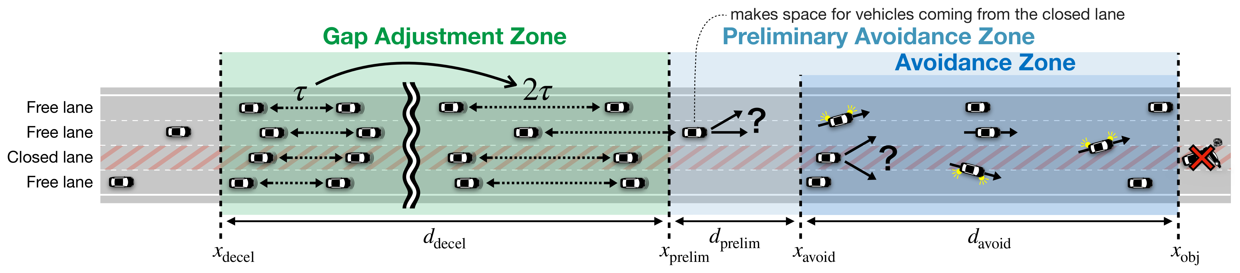
3.2. Basic Strategy

Each vehicle determines its behavior according to the distance d = x obj x between the position of the obstacle x obj and its position x. To this end, we define zones before the obstacle, as shown in Figure 3. If a vehicle is in the lane that is closed by the obstacle (referred to as the closed lane) and the distance to the obstacle, d, satisfies 0 < d d avoid (referred to as the avoidance zone), it attempts to change lanes. If a vehicle is in the lane where the obstacle does not exist (referred to as the free lane) and d satisfies 0 < d d avoid + d prelim (referred to as the preliminary avoidance zone), it attempts to change lanes. If d satisfies d avoid + d prelim < d d avoid + d prelim + d decel (referred to as the gap adjustment zone), a vehicle increases the time headway to make space to accommodate vehicles entering from the neighboring lane.
Let us describe the notion of the preliminary avoidance zone. In this zone, vehicles in the free lane attempt to change lanes in order to distribute traffic. Note that the length of the preliminary avoidance zone is larger than the avoidance zone. This design is because vehicles in the free lanes need to change lanes earlier to make space so that vehicles in the closed lane can change lanes. Note that the preliminary avoidance zone is unnecessary when a free lane does not have a neighboring free lane. For example, when the center lane of a three-lane road is closed, vehicles in a free lane, i.e., the left edge or the right edge, cannot move to another free lane. Thus, the preliminary avoidance zone is unnecessary in this case, and d prelim = 0 .

3.3. Obstacle Detection Notification

When a CV detects an obstacle using its sensors (e.g., cameras or LiDAR), it broadcasts an obstacle detection notification message, which includes the obstacle’s position and the index of the closed lane, to the vehicles in all lanes behind it. In this paper, we assume the index starts from the right edge lane. The index of the right edge lane of a three-lane road is 0, and that of the center lane is 1. We assume that the message is disseminated to vehicles on the same road within a few kilometers range using a flooding protocol with appropriate optimization. A vehicle that detects an obstacle will continue to broadcast the same message periodically until it passes the obstacle. Each obstacle detection notification message is valid during a given period of validity, e.g., 60 s. If the obstacle is cleared, no vehicle broadcasts obstacle detection notification messages, and thus the following vehicles are not notified. Therefore, vehicles can know the obstacle has been cleared indirectly by not receiving obstacle detection notification messages. Then traffic flow returns to normal. However, the obstacle avoidance operation of each vehicle continues until the end of the validity period of the last received obstacle detection notification message.

3.4. Adjusting Time Headway

All vehicles in the gap adjustment zone control their speed to double the normal time headway so that they can smoothly change lanes when they enter the (preliminary) avoidance zone. The time headway is the time from when a vehicle in front of the ego vehicle passes a point to when the ego vehicle passes the same point. Each vehicle in the gap adjustment zone calculates its deceleration based on its current speed v so that its time headway is double the normal time when it reaches position x h . x h for vehicles in the closed lane is x avoid , whereas x h for vehicles in the free lane is x prelim . To maintain ride comfort, the acceleration value is kept equal or larger than a comfort . A vehicle may not be able to extend the time headway to the ideal value before it reaches x h , where it intends to finish the adjustment of time headway. In such a case, it will continue decelerating at a comfort until its time headway reaches the ideal value.

3.5. Adaptive Lane Change

When avoiding an obstacle, a vehicle in a lane other than the outermost lanes has two candidate lanes to which it moves. A vehicle in the closed lane can choose either lane to its immediate left or right. On the other hand, a vehicle in the free lane can choose to change lanes to move away from the obstacle or go straight ahead. In our scheme, the destination lane for these vehicles is selected according to Strategy 1 (avoiding congested lanes) and Strategy 2 (adjusting the balance among lanes).
Strategy 1: Avoiding congested lanes: As shown in Figure 4a, the ego vehicle, a vehicle that will change lanes, evaluates the number of vehicles between itself and the obstacle in each destination candidate lane. First, it counts the number of vehicles in front of itself in each lane and in its communication range on the basis of the number of unique vehicle IDs included in the packets sent from the vehicles. Let a and b be indices of the destination candidate lanes and let m a and m b be the number of vehicles in each of the lanes, respectively. If either the ratio of m a or m b to the sum of m a and m b exceeds a predefined threshold L (e.g., 0.6), the vehicle regards the lane as congested and moves to another lane to balance the traffic of the lanes ahead. In other words, lane i   (   { a , b } ) that satisfies m i / m a + m b > L cannot be a candidate destination lane. If neither candidate is selected, the vehicle uses Strategy 2 to determine the destination lane.
Strategy 2: Adjusting the balance among lanes: As shown in Figure 4b, a vehicle determines a destination lane in such a way that the number of vehicles in each free lane will have the same amount of traffic. First, the vehicle counts the number of vehicles in each lane behind itself and its communication range on the basis of the number of unique vehicle IDs included in the packets sent from the vehicles. Let us assume that the road has n lanes ( n 1 ), then the index of each lane is i   (   { 0 ,   1 ,   ,   n 1 } ) , the number of counted vehicles in each lane is m i , and M = i = 0 n 1 m i . If the counted vehicles are evenly distributed among the n 1 free lanes, the ideal number of vehicles per free lane is M / ( n 1 ) . To adjust the number of vehicles in each lane to be closer to this ideal number, the probability that a vehicle moves from lane i to lane j P i j   ( j { i 1 ,   i ,   i + 1 } ) in either direction from each lane is calculated in three steps as follows, where the index of the closed lane is denoted by c.
The candidates of a destination lane of a vehicle are limited by its current lane. Vehicles in the rightmost lane cannot move right, vehicles in the leftmost lane cannot move left lane, vehicles in the closed lane cannot go straight ahead, and vehicles always change lanes to the lane farther from the obstacle. Thus,
P 0 1 = 0 ,       P n 1 n = 0 ,       P c c = 0 ,
P i i + 1 = 0 ,       i { 0 ,   1 ,   ,   c 1 } ,
P i i 1 = 0 ,       i { c + 1 ,   c + 2 ,   ,   n 1 } .
Next, we calculate the lane change probability to balance the traffic among lanes. The number of vehicles that should move to lane j is calculated on the basis of the difference between the number of vehicles m j and the ideal number of vehicles M / ( n 1 ) . In this case, P j j + ( j i ) × m j vehicles in lane j should move to another lane. Accordingly, the difference between the number of vehicles in lane j and the ideal number of vehicles in each lane will be M / ( n 1 ) ( 1.0 P j j + ( j i ) ) m j . Then, we calculate the probability P i j so that the number of vehicles changing lanes from lane i to lane j can be M / ( n 1 ) ( 1.0 P j j + ( j i ) ) m j . Thus,
P i i 1 = M / ( n 1 ) ( 1.0 P i 1 i 2 ) m i 1 m i ,       i { 1 ,   2 ,   ,   c } ,
P i i + 1 = M / ( n 1 ) ( 1.0 P i + 1 i + 2 ) m i + 1 m i ,       i { c ,   c + 1 ,   ,   n 2 } .
However, if P i j > 1.0 , then P i j = 1.0 , and if P i j < 0.0 , then P i j = 0.0 .
Finally,
P i i = 1.0 ( P i i 1 + P i i + 1 ) ,       i { 0 ,   1 ,   ,   c 1 ,   c + 1 ,   ,   n 1 } .
Table 1 summarizes the movement probabilities of vehicles in each lane when lane c in a n-lane road is closed. As a concrete example, Table 2 summarizes the movement probabilities in each lane when the rightmost lane in a three-lane road is closed. In this case, a vehicle in the center lane moves to the left lane with a probability ( M / 2 m 2 ) / m 1 and goes straight ahead with a probability ( M / 2 m 0 ) / m 1 .

4. Simulation Model

To confirm the effectiveness of the proposed scheme, we conducted simulations using the traffic flow simulator SUMO 1.6.0 [8] and its external control interface TraCI [23].

4.1. Environment Settings

As shown in Figure 5, we assume a situation where an obstacle arises on a one-way straight highway road with two or three lanes. We assume that the road length is 2   km , and a vehicle playing the role of the obstacle enters the road at 20   s and stops at a point 1950   m from the starting point. Vehicles enter the road in accordance with a Poisson arrival model, and their entry lane is chosen randomly. Vehicles start at an initial speed of 16.7   m / s and move at a speed limit of 33.3   m / s . The V2V communication range is assumed to be 300   m , considering that the dedicated short range communications (DSRC) communication range in real environments is around 300   m [24]. Moreover, it is assumed that CVs frequently broadcast driving information messages (e.g., position and speed) and they know the positions of other CVs within this range. In the proposed scheme, the number of vehicles in each lane is counted within this range. If a vehicle detects an obstacle, it broadcasts a notification message at 0.2   s intervals until it passes the obstacle.
The communications are simplified in the simulations. It is assumed that obstacle detection notification messages are immediately delivered to all following CVs within 1.5   km from the source of the message by multi-hop communication. Table 3 summarizes the simulation parameter values.
Table 3. Simulation parameters.
ParametersValues
Simulation time 500.0   s
Time step length 0.05   s
d avoid (avoidance zone size)10–500 m
d prelim (preliminary avoidance zone size)0–300 m
d decel (gap adjustment zone size)0–1000 m
a comfort for adjusting time headway 2.94   m / s 2 ( 0.3   G ) [25]
Threshold L for avoiding congested lanes0.6
Available sensing range 50   m [26]
V2V communication range 300   m [24]
Traffic load input value for 2-lane scenario720–3600 vehicles/h
Traffic load input value for 3-lane scenario720–5400 vehicles/h
CV penetration ratio0.0–1.0
Broadcast interval 0.2   s
Validity period of the obstacle information 60.0   s
Vehicle length, vehicle width 4.47   m , 1.795   m
Min. inter-vehicular distance 2.5   m
Regular inter-vehicular gap ( τ ) 2.0   s
Gap open ratio2.0
Lane change duration 3.0   s
LC2013 lane change mode1621
Initial speed, road speed limit 16.7   m / s , 33.3   m / s
Max. acceleration, max. deceleration 2.9   m / s 2 , 7.5   m / s 2

4.2. Lane-Changing Model

Vehicles are passenger cars that follow the default car-following model (Krauss) [27] of SUMO. Vehicles change lanes according to the default lane-changing model (LC2013) [28] of SUMO. In this model, vehicles change lanes in accordance with the following four motivations:
  • Strategic change: Changing lanes to reach a destination (e.g., moving to the left lane to make a left turn).
  • Cooperative change: Changing lanes to help another vehicle change lanes (e.g., changing lanes to make space for merging vehicles at a merge point).
  • Tactical change: Changing lanes to move faster (e.g., overtaking).
  • Regulatory change: Changing lanes to comply with regulations and laws (e.g., changing lanes to avoid driving continuously in an overtaking lane).
In LC2013, each motivation setting can be controlled by changing the lane change mode. Basically, vehicles move in lane change mode 1621, where the four motivations, collision avoidance, and safety-gap enforcement functions, are enabled. If a vehicle is aware of the obstacle according to its onboard sensor data or an obstacle detection notification message, it changes its mode to 512, wherein the four motivations are disabled. In this mode, we control the vehicle’s lane changes with the changeLane command provided by SUMO. We also control the vehicle’s acceleration for opening the inter-vehicular gap (thus increasing the time headway) in the gap adjustment zone by using the openGap command. For openGap, we configured the target time headway parameter 2 τ (i.e., double the normal value.), the time required for opening a gap v / x h x , and the minimum acceleration a comfort . In this study, we set a comfort at 2.94   m / s 2 ( 0.3   G ) based on [25], deceleration that does not degrade ride comfortability.
In the simulations, the “–lanechange.overtake-right” option of SUMO is set to True in order to allow overtaking from the right of an obstacle on the center lane of the three-lane road.

4.3. Vehicle Detection Model

The available sensing range of the on-board sensors is assumed to be 50   m , considering that the available object detection range of onboard LiDARs is from a few meters to 200   m [26]. The simulations consider occlusion (a state in which an object in the foreground conceals an object in the background), that is, they consider line of sight. As shown in Figure 6, each vehicle model has a center point, eight measurement points, four vertices and the midpoints of the sides of a rectangle representing the vehicle body. A vehicle can detect a target vehicle within the available sensing range if there are two or more line segments connecting its center point and each measurement point of the target vehicle that does not intersect with the body of another vehicle.

4.4. Vehicle Behavior Models

To investigate the performance of our scheme, we used the five vehicle behavior models listed below.
  • Proposed_Full: CVs follow the proposed scheme.
  • Proposed_NoAdaptive: Simplified version of Proposed_Full. Vehicles randomly select a destination lane from two destination lane candidates.
  • Proposed_NoPrelim: Simplified version of Proposed_Full. d prelim = 0 .
  • Proposed_NoGapOpen: Simplified version of Proposed_Full. The function of adjusting time headway is disabled.
  • Manual: Human-driven vehicle (i.e., NCV) model. Vehicles change lanes to avoid obstacles only when they directly detect an obstacle. If there are lanes on both sides, vehicles in the closed lane randomly select a destination lane.

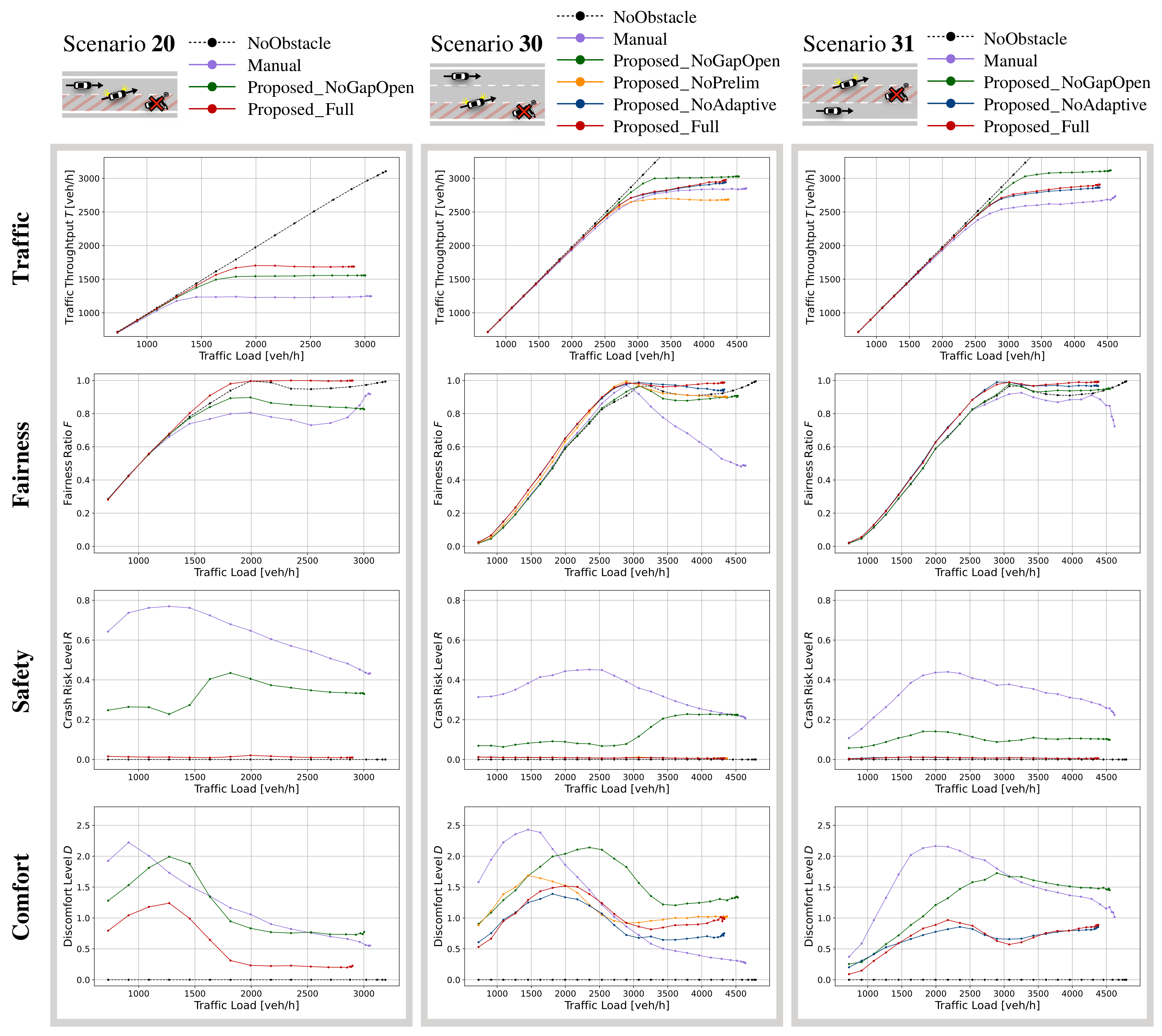
4.5. Performance Metrics

To evaluate the effectiveness of the proposed scheme from the four perspectives of traffic, fairness, safety, and comfort, we defined the following performance metrics.

4.5.1. Traffic

Traffic was evaluated in terms of the number of vehicles per second overtaking the obstacle. The traffic throughput T in each simulation is given by
T = M t end t closed ,
where t end is the simulation end time, t closed is the time at which the obstacle vehicle stops, and M is the number of vehicles arriving at the endpoint between t closed and t end .

4.5.2. Fairness

Fairness was evaluated with the difference in traffic between the most congested and the least congested lanes. Let the number of vehicles that was in lane i when it was 600   m behind the obstacle and arrived at the endpoint be m i . The fairness ratio F in each simulation is defined as follows:
F = min { m 0 ,   m 1 ,   ,   m n 1 } max { m 0 ,   m 1 ,   ,   m n 1 } .
Note that 600   m is the maximum of the sum of d avoid and d prelim in the simulation setting.

4.5.3. Safety

Safety was evaluated with the Time To Collision (TTC), i.e., the time left before two vehicles collide. The TTC of a vehicle combination i at time t with respect to a leading vehicle i 1 on the same path is given by
TTC i ( t ) = x i 1 ( t ) x i ( t ) l i v i ( t ) v i 1 ( t )         v i ( t ) > v i 1 ( t ) ,
where v, x, and l denote speed, position, and length of a vehicle, respectively [29]. Since a small TTC value corresponds to a high crash risk [30], we obtained the crash risk level R in each simulation as follows:
R = P ( TTC min 5 ) ,
where TTC min   [ s ] is the minimum TTC of each vehicle arriving at the endpoint.

4.5.4. Comfort

Comfort was evaluated by the degree of discomfort of passengers proposed by Wang et al. [31]. They showed that a passenger’s ride comfort due to speed fluctuations depends on both acceleration and jerk (change in acceleration rate) and used these factors to derive a discomfort index. The discomfort level d ( t ) at time t is given by
d ( t ) = β 1 a p + ( t ) + β 2 a p ( t ) + β 3 j r + ( t ) + β 4 j r ( t ) ,
where a p + ( t )   [ m / s 2 ] is the positive peak value of acceleration between t 3   [ s ] and t, a p ( t )   [ m / s 2 ] is the absolute value of the negative peak value of acceleration between t 3   [ s ] and t, j r + ( t )   [ m / s 3 ] is the effective value when the average jerk between t 3   [ s ] and t is positive, and j r ( t )   [ m / s 3 ] is the effective value when the average jerk between t 3   [ s ] and t is negative. In [31], two combinations of coefficients for each term were derived, one for a passenger in a resting posture and the other for a passenger in a reading posture. In this study, we used the coefficient combination for the reading posture, β 1 = 0.19 , β 2 = 0.53 , β 3 = 0.27 , and β 4 = 0.34 . Since the units of acceleration and jerk are different, the definition of d ( t ) is tricky, and the unit of d ( t ) generally cannot be given. We treat d ( t ) as a unitless number as [31] does.
To calculate d using Equation (11), we calculated the acceleration by firstly applying the least-squares method to smooth the speed samples obtained from SUMO [32] and differentiating the result numerically using the central difference method. Then, we calculated the jerk by differentiating the acceleration in the same way. We calculated the discomfort per vehicle by averaging the cumulative discomfort of all vehicles arriving at the endpoint. Since we wanted to focus on cases where the passengers feel high levels of discomfort, we obtained the discomfort level D in each simulation as follows:
D = 1 | A | i A t departure , i t arrival , i max { d i ( t ) d thresh ,   0 } d t ,
where A is the set of vehicles arriving at the endpoint, t departure , i is the time when vehicle i departed from the warm-up zone, t arrival , i is the time when vehicle i arrived at the endpoint, and d thresh is a threshold of high discomfort. In this study, d thresh = 4 .

5. Simulation Results and Discussion

We conducted simulations of three scenarios, named 20, 30, and 31. In Scenario 20, there is a 2-lane road, and lane 0 (right edge lane) is closed. In Scenario 30, there is a 3-lane road, and lane 0 (right edge lane) is closed. In Scenario 31, there is a 3-lane road, and lane 1 (center lane) is closed. For all scenarios, we conducted 100 simulations with different random seeds. All of the plotted points on the graphs are average values. Figure 7 shows the some snapshots of simulations.

5.1. Effect of Cooperative Lane Change

Figure 8 graphs the cumulative distribution function (CDF) for each metric when the traffic load is low (2880 vehicles/h for Scenario 20 and 4320 vehicles/h for Scenarios 30 and 31) or high (1440 vehicles/h for Scenario 20 and 2160 vehicles/h for Scenarios 30 and 31). Figure 9 graphs the comprehensive evaluation values for each metric under different traffic loads, from low traffic loads to the maximum traffic loads that can work in simulation in the SUMO simulator. NoObstacle represents the case when there are no obstacles, i.e., the ideal road condition. Thus, the closer the metric value of the vehicle behavior model is to NoObstacle, the better the model becomes.
First, let us focus on the case of the low traffic load. From Figure 9, we can see that there is little difference in the traffic throughput at low traffic load among the vehicle behavior models. However, from Figure 8, we can see that there is a large difference in the CDF of the minimum speeds at low traffic load among the vehicle behavior models. This is because the vehicle behavior of overtaking the obstacle significantly differs among the models, even if the road is not congested. In Manual, the minimum speed of each vehicle is smaller than in the other models because rapid deceleration is required to overtake the obstacle, as each vehicle can start changing lanes only after it directly detects the obstacle and thus it has to finish lane changes within a short distance. That rapid deceleration to avoid a collision can be seen in the results of the CDF of the minimum TTC and the CDF of the maximum jerk in Figure 8. On the other hand, the models based on the proposed scheme are better than Manual in terms of traffic throughput, safety, and comfort level. This is because sharing information about the obstacle through V2V communication allows them to adjust their speed and change lanes in advance, preventing rapid deceleration. None of the models caused traffic jams; thus, they all have similar fairness.
Next, we focus on the case of the high traffic load. From Figure 9, we can see that there is a large difference among the models in each metric at the high traffic load. Therefore, we discuss each vehicle behavior model below.
Manual: In Scenarios 20 and 31, Manual has lower traffic throughput and lower comfort level than the other models. This is because all vehicles in the free lanes are heavily affected by the traffic that moves from the closed lane, resulting in traffic jams in all lanes. On the other hand, in Scenario 30, Manual has similar traffic throughput to the other models and achieves the highest comfort level. However, it has the worst fairness of traffic throughput among lanes. This is because chronic traffic jams occur in lanes 0 and 1 in Scenario 30. Here, lane 2 is the farthest from the closed lane (lane 0), and vehicles in lane 2 are mostly unaffected by lane changes from the closed lane and hence, they keep moving quickly. On the other hand, vehicles in lane 1 need to decelerate to accommodate vehicles changing lanes from the closed lane. The difference in speed between vehicles in lanes 2 and 1 increases; thus, vehicles in lane 1 find it hard to move to lane 2. Therefore, the number of acceleration changes is reduced by the chronic traffic jams in lanes 0 and 1. That is, vehicles in lane 2 keep moving quickly, and vehicles in lanes 0 and 2 move slowly; thus, the discomfort level is very low. Additionally, in Scenario 30, lane 2 has much higher traffic throughput than lanes 0 and 1; thus, the total traffic throughput improves but fairness deteriorates compared with the other scenarios. This can be seen in Figure 8, where there are large differences in the minimum speed and in the travel times.
Proposed_NoGapOpen: In Scenarios 30 and 31, Proposed_NoGapOpen has the highest traffic throughput. This is because vehicles do not decelerate to adjust their time headway in this model, so they tend to keep moving at high speed even when changing lanes, thus increasing traffic throughput. On the other hand, the safety and comfort levels of this model are low. This is because the vehicles do not adjust their time headway, so they need to decelerate rapidly in a short time.
Proposed_NoPrelim: In Scenario 30, Proposed_NoPrelim shows little difference in fairness, safety, and comfort level compared with Proposed_Full, but has lower traffic throughput. This is because in Proposed_Full, vehicles in the free lane change lanes first in the preliminary avoidance zone to make space for vehicles in the closed lane to change lanes in the avoidance zone, and this reduces the number of times they need to slow down, compared with the case of Proposed_NoPrelim.
Proposed_NoAdaptive: Proposed_NoAdaptive shows little difference compared with Proposed_Full in all metrics. The reason is as follows. When the CV penetration ratio is 100%, temporary congestion around the obstacle rarely occurs because vehicles in the closed lanes change lanes with plenty of time to spare when Proposed_NoAdaptive and Proposed_Full are used. Therefore, strategy 1 (avoiding congested lane) has little chance to work. Additionally, the amount of traffic load input is the same in all lanes. Thus, the probabilities of changing lanes from the center lane to the left lane and from the center lane to the right calculated in Proposed_Full are the same (50%) in Scenario 31. The results are the same for Proposed_NoAdaptive when the lane is randomly selected. Note that the effect of the adaptive lane change can be seen when the CV penetration ratio is less than 100%. For scenarios with four or more lanes, Strategy 2 is expected to be more effective and provide an advantage over the random decision case.
Proposed_Full: Proposed_Full achieves sufficiently high total traffic throughput in all scenarios. In addition, it achieves very high fairness, safety, and comfort level in all scenarios. However, it has lower traffic throughput than Proposed_NoGapOpen in Scenarios 30 and 31, but higher traffic throughput in Scenario 20. This is because the control of doubling the time headway of vehicles in all three lanes is excessive, resulting in lower traffic throughput. Thus, it is expected that as the ratio of closed lanes to the total roadway lanes becomes smaller, the control of doubling the time headway of all vehicles will become excessive, and a lower traffic throughput will result. There is thus room for improving our method in the future.
From these discussions, we can summarize the effect of the proposed cooperative lane change as follows:
  • Sharing information about the obstacle through V2V communication allows vehicles to adjust their speed and change lanes in advance, preventing rapid deceleration.
  • Adjusting the time headway of vehicles in advance is effective at significantly improving safety and comfort level in obstacle avoidance.
  • Shifting the lane change timing between vehicles in the closed lane and vehicles in the free lane by introducing a preliminary avoidance zone is effective in facilitating obstacle avoidance.
  • The proposed scheme achieves sufficiently high traffic throughput without degrading fairness, safety, or comfort level in the most balanced way. Note that we assume that vehicles’ microscopic operation depends on the lane change model of SUMO. Therefore, the performance of the proposed scheme may vary depending on trajectory planning.

5.2. Impact of the CV Penetration Ratio

Next, let us investigate the impact of the CV penetration ratio. Figure 10 shows the simulation results when using Proposed_Full for various values of the CV penetration ratio. We assume that the NCVs follow Manual.
Overall, all metrics tend to become worse as the CV penetration ratio declines. However, traffic throughput and comfort level tend to improve above 50% the CV penetration ratio. These characteristics show that when the CV penetration is around 50%, obstacle avoidance is less smooth than when either CVs or NCVs are dominant. This can be explained as follows. As the CV penetration ratio becomes smaller, more vehicles in the closed lane have difficulty in completing a lane change, resulting in more frequent rapid deceleration and traffic jams around the obstacle, thereby degrading the traffic throughput and comfort level. On the other hand, as the CV penetration ratio becomes smaller, that is, as more vehicles do not adjust their time headway, they tend to maintain a high speed, and, thus, the traffic throughput increases. Even if some vehicles have a high discomfort level, if many vehicles overtake the obstacle at high speed, the average discomfort will be low. As a result of these two phenomena, as the CV penetration ratio approaches 50%, traffic throughput and comfort level deteriorate.
We can see that the 10% CV penetration ratio improves the fairness of the traffic throughput compared with the 0% CV penetration ratio in Scenario 30. This is because even with a 10% ratio, the CVs act to accommodate lane-change vehicles by adjusting their time headway, thereby restraining chronic traffic jams in lane 0 (closed lane) and lane 1.

5.3. Impact of the Zone Sizes

Finally, let us investigate the impact of the zone sizes of the proposed scheme. Figure 11 shows simulation results when the sizes of the avoidance zone, preliminary avoidance zone, and gap adjustment zone are varied in Scenario 30. Our proposed method focuses on the vehicles moving in the wide range behind the obstacle. Wide range control may have a negative side effect on the following traffic. For example, deceleration for changing lanes may affect the behavior of vehicles to adapt to road structures, such as ramps and intersections. Therefore, a shorter zone is preferable as long as safe, smooth, and fair obstacle avoidance can be assured.
Avoidance zone: If the avoidance zone is too small, vehicles in the closed lane cannot change lanes. Therefore, the size of the avoidance zone ( d avoid ) should be sufficient for vehicles in the closed lane to accomplish a lane change. Simulation results show that traffic throughput, fairness, and comfort level deteriorate when d avoid < 250   m . On the other hand, all metrics are stable when d avoid 250   m . Consequently, we can conclude that a suitable size of the avoidance zone is 250   m or more.
Preliminary avoidance zone: If a vehicle in the closed lane and a vehicle in a free lane begin attempting to change lanes at the same point in time, the vehicle in the closed lane may be able to change lanes faster than the vehicle in the free lane. In this case, the vehicle density in the free lane temporarily increases, and vehicles in the free lane will be forced to decelerate. Therefore, the size of the preliminary avoidance zone ( d prelim ) should be sufficient to shift the lane-change timings for vehicles in the closed lane and the lane change timing for vehicles in the free lane. Simulation results show that traffic throughput improves when d prelim 30   m . However, the fairness and comfort level deteriorate when d prelim > 100   m . This result can be explained as follows. If the size of the preliminary avoidance zone is too large, there is too much of a time lag between the lane change of the vehicle in the free lane and the lane change of the vehicle in the closed lane, and the following vehicle accelerates to shorten the long inter-vehicular gap made by the lane changes of the vehicles in the free lane. As a result, when the vehicle in the closed lane starts to change lanes, there will be insufficient space for it to change lanes smoothly, and the vehicles need to decelerate. Thus, the fairness of the traffic throughput and comfort level deteriorate with frequent deceleration in the lane next to the closed one. Consequently, we can conclude that a suitable size of the preliminary avoidance zone is 30–100 m.
Gap adjustment zone: In the gap adjustment zone, vehicles do not decelerate rapidly to double the time headway within a short time because of the minimum acceleration a comfort . If the gap adjustment zone is too short, vehicles cannot double the time headway. Therefore, the size of the gap adjustment zone ( d decel ) should be sufficient to double the time headway without reducing ride comfort. Simulation results show that traffic throughput and fairness deteriorate when d decel < 200   m . In addition, traffic throughput deteriorate when d decel > 600   m . This is because as the gap adjustment zone becomes larger, the travel time of vehicles at low speed becomes longer. Consequently, we can conclude that a suitable size of the gap adjustment zone is 200–600 m.

6. Conclusions

We proposed a rule-based cooperative lane change control scheme to avoid a suddenly appearing obstacle on three or more-lane roads. In this scheme, a vehicle that detects the obstacle uses multi-hop V2V communication to share the obstacle’s position with vehicles behind it in a wide range. In addition, this scheme smoothly distributes the traffic to free lanes by making vehicles approaching the obstacle adjust their time headway and select the destination lane according to the obstacle’s position and number of vehicles in each lane estimated from beacon messages broadcast by each CV. Simulation results show that the proposed scheme achieves sufficiently high traffic throughput without degrading fairness, safety, or comfort level. Even with only a 10% CV penetration ratio, the proposed scheme works to avoid chronic traffic jams and improve the fairness among lanes. In the future, we plan to conduct simulation evaluations and performance improvements on roads with more than four lanes or when obstacles close multiple lanes. We also plan to use a realistic wireless communication simulation model and develop a machine-learning-based obstacle-avoidance method.

Author Contributions

Conceptualization, S.A. and S.I.; Data curation, S.A.; Formal analysis, S.A. and S.I.; Funding acquisition, S.I.; Investigation, S.A.; Methodology, S.A. and S.I.; Project administration, S.I.; Resources, S.I.; Software, S.A.; Supervision, S.I.; Validation, S.A. and S.I.; Visualization, S.A.; Writing—original draft, S.A.; Writing—review and editing, S.I. All authors have read and agreed to the published version of the manuscript.

Funding

This research received no external funding.

Institutional Review Board Statement

Not applicable.

Informed Consent Statement

Not applicable.

Data Availability Statement

Not applicable.

Conflicts of Interest

The authors declare no conflict of interest.

References

  1. National Highway Traffic Safety Administration, Vehicle-to-Vehicle Communication. Available online: https://www.nhtsa.gov/technology-innovation/vehicle-vehicle-communication (accessed on 16 August 2022).
  2. Persaud, B.; Yagar, S.; Brownlee, R. Exploration of the Breakdown Phenomenon in Freeway Traffic. J. Transp. Res. Rec. 1998, 1634, 64–69. [Google Scholar] [CrossRef]
  3. Sugiyama, Y.; Fukui, M.; Kikuchi, M.; Hasebe, K.; Nakayama, A.; Nishinari, K.; Tadaki, S.; Yukawa, S. Traffic jams without bottlenecks-experimental evidence for the physical mechanism of the formation of a jam. New J. Phys. 2008, 10, 033001. [Google Scholar] [CrossRef]
  4. Google Maps. Available online: https://www.google.com/maps/ (accessed on 16 August 2022).
  5. Waze: Driving Directions, Live Traffic & Road Conditions Updates. Available online: https://www.waze.com/ja/live-map/ (accessed on 16 August 2022).
  6. Vehicle Information and Communication System. Available online: https://www.vics.or.jp/en/ (accessed on 16 August 2022).
  7. Ishihara, S. Cooperative Lane Change Control for Sudden Obstacle Avoidance on a Multilane Road. In Proceedings of the ITS Symposium, Ishikawa, Japan, 12–13 December 2019. [Google Scholar]
  8. Simulation of Urban Mobility (SUMO). Available online: http://sumo.dlr.de/wiki/ (accessed on 16 August 2022).
  9. Asano, S.; Ishihara, S. Rule-Based Cooperative Lane Change Control to Avoid a Sudden Obstacle in a Multi-Lane Road. In Proceedings of the 2022 IEEE 95th Vehicular Technology Conference, Helsinki, Finland, 19–22 June 2022. [Google Scholar]
  10. Desiraju, D.; Chantem, T.; Heaslip, K. Minimizing the Disruption of Traffic Flow of Automated Vehicles During Lane Changes. IEEE Trans. Intell. Transp. Syst. 2016, 16, 1249–1258. [Google Scholar] [CrossRef]
  11. Wang, D.; Hu, M.; Wang, Y.; Wang, J.; Qin, H.; Bian, Y. Model predictive control-based cooperative lane change strategy for improving traffic flow. Adv. Mech. Eng. 2016, 8, 1–17. [Google Scholar] [CrossRef]
  12. Luo, Y.; Yang, G.; Xu, M.; Qin, Z.; Li, K. Cooperative Lane-Change Maneuver for Multiple Automated Vehicles on a Highway. Automot. Innov. 2019, 2, 157–168. [Google Scholar] [CrossRef]
  13. Li, T.; Wu, J.; Chan, C.Y.; Liu, M.; Zhu, C.; Lu, W.; Hu, K. A Cooperative Lane Change Model for Connected and Automated Vehicles. IEEE Access 2020, 8, 54940–54951. [Google Scholar] [CrossRef]
  14. CAR 2 CAR Communication Consortium (C2C-CC), Guidance for Day 2 and Beyond Roadmap. Available online: https://www.car-2-car.org/fileadmin/documents/General_Documents/C2CCC_WP_2072_RoadmapDay2AndBeyond.pdf (accessed on 16 August 2022).
  15. Gunther, H.; Trauer, O.; Wolf, L. The Potential of Collective Perception in Vehicular Ad-Hoc Networks. In Proceedings of the 2015 14th International Conference on ITS Telecommunications, Copenhagen, Denmark, 2–4 December 2015. [Google Scholar]
  16. Federal Highway Administration (FHWA), CARMA Program Overview. Available online: https://highways.dot.gov/research/operations/CARMA (accessed on 16 August 2022).
  17. Tiernan, T.; Bujanovic, P.; Azeredo, P.; Najm, W.G.; Lochrane, T. CARMA Testing and Evaluation of Research Mobility Applications; U.S. Department of Transportation, Federal Highway Administration: San Francisco, CA, USA, 2019.
  18. Ding, J.; Li, L.; Peng, H.; Zhang, Y. A Rule-Based Cooperative Merging Strategy for Connected and Automated Vehicles. IEEE Trans. Intell. Transp. Syst. 2020, 21, 3436–3446. [Google Scholar] [CrossRef]
  19. Jing, S.; Hui, F.; Zhao, X.; Rios-Torres, J.; Khattak, A.J. Cooperative Game Approach to Optimal Merging Sequence and on-Ramp Merging Control of Connected and Automated Vehicles. IEEE Trans. Intell. Transp. Syst. 2019, 20, 4234–4244. [Google Scholar] [CrossRef]
  20. Multi-Car Collision Avoidance (MuCCA). Available online: https://mucca-project.co.uk (accessed on 16 August 2022).
  21. Wartnaby, C.; Bellan, D. Decentralised Cooperative Collision Avoidance with Reference-Free Model Predictive Control and Desired Versus Planned Trajectories. arXiv 2019, arXiv:1904.07053. [Google Scholar]
  22. Bae, S.Y.; Saxena, D.M.; Nakhaei, A.; Choi, C.; Fujimura, K.; Moura, S.J. Cooperation-Aware Lane Change Maneuver in Dense Traffic based on Model Predictive Control with Recurrent Neural Network. In Proceedings of the 2020 American Control Conference (ACC), Denver, CO, USA, 1–3 July 2020. [Google Scholar]
  23. Wegener, A.; Piorkowski, M.; Raya, M.; Hellbruck, H.; Fischer, S.; Hubaux, J. TraCI: An Interface for Coupling Road Traffic and Network Simulators. In Proceedings of the 11th Communications and Networking Simulation Symposium (CNS), Ottawa, ON, Canada, 14–17 April 2008. [Google Scholar]
  24. Xu, Q.; Mak, T.; Ko, J.; Sengupta, R. Vehicle-to-vehicle safety messaging in DSRC. In Proceedings of the 1st ACM International Workshop on Vehicular Ad Hoc Networks, Philadelphia, PA, USA, 1 October 2004. [Google Scholar]
  25. Deligianni, S.; Quddus, M.; Morris, A.; Anvuur, A.; Reed, S. Analyzing and Modeling Drivers’ Deceleration Behavior from Normal Driving. Transp. Res. Rec. J. Transp. Res. Board 2017, 2663, 134–141. [Google Scholar] [CrossRef]
  26. Texas Instruments. An Introduction to Automotive LIDAR. Available online: https://www.ti.com/lit/wp/slyy150a/slyy150a.pdf (accessed on 16 August 2022).
  27. Krauss, S.; Wagner, P.; Gawron, C. Metastable States in a Microscopic Model of Traffic Flow. Phys. Rev. E 1997, 55, 5597–5602. [Google Scholar] [CrossRef]
  28. Erdmann, J. SUMO’s Lane-Changing Model. In Modeling Mobility with Open Data; Lecture Notes in Mobility; Springer: Berlin/Heidelberg, Germany, 2015; pp. 105–123. [Google Scholar]
  29. Minderhoud, M.M.; Bovy, P.H.L. Extended Time-To-Collision Measures for Road Traffic Safety Assessment. Accid. Anal. Prev. 2001, 33, 89–97. [Google Scholar] [CrossRef]
  30. Vogel, K. A Comparison of Headway and Time to Collision as Safety Indicators. Accid. Anal. Prev. 2003, 35, 427–433. [Google Scholar] [CrossRef]
  31. Wang, F.; Segawa, K.; Inooka, H. A Study of the Relationship between the Longitudinal Acceleration/Deceleration of Automobiles and Ride Comfort. Jpn. J. Ergon. 2000, 36, 191–200. [Google Scholar]
  32. Savitzky, A.; Golay, M.J.E. Smoothing and Differentiation of Data by Simplified Least Squares Procedures. Anal. Chem. 1964, 36, 1627–1638. [Google Scholar] [CrossRef]
Figure 1. Obstacle avoidance using V2V communication. (a) Avoidance strategy when the obstacle’s existence cannot be shared via V2V communication. (b) Avoidance strategy when vehicles share the obstacle’s existence and location using V2V communication.
Applsci 12 08528 g001
Figure 2. Control rules based on distance between an obstacle and approaching vehicles on a two-lane road.
Applsci 12 08528 g002
Figure 3. Control rules based on distance between an obstacle and approaching vehicles on a road with three or more lanes.
Applsci 12 08528 g003
Figure 4. Adaptive lane change. (a) Strategy 1: Avoiding congested lanes. (b) Strategy 2: Adjusting the balance among lanes.
Applsci 12 08528 g004
Figure 5. Traffic flow simulation in SUMO.
Applsci 12 08528 g005
Figure 6. Vehicle detection model in the simulation.
Applsci 12 08528 g006
Figure 7. Snapshots of simulations. The green box indicates an obstacle. Red boxes are cars that have detected the obstacle directly. (a) Simulations of obstacle avoidance in Scenario 20. (b) Simulations of obstacle avoidance in Scenario 30.
Applsci 12 08528 g007
Figure 8. Simulation results for each vehicle behavior model under fixed traffic loads, d avoid = 300   m , d prelim = 100   m , d decel = 500   m , CV penetration ratio = 1.0.
Applsci 12 08528 g008
Figure 9. Simulation results for each vehicle behavior model under different traffic loads, d avoid = 300   m , d prelim = 100   m , d decel = 500   m , CV penetration ratio = 1.0.
Applsci 12 08528 g009
Figure 10. Simulation results showing impact of CV penetration ratio under different traffic loads, d avoid = 300   m , d prelim = 100   m , d decel = 500   m .
Applsci 12 08528 g010
Figure 11. Simulation results showing impact of zone sizes under fixed traffic loads, CV penetration ratio = 1.0.
Applsci 12 08528 g011
Table 1. Movement probabilities in n-lanes when lane c is closed.
Lane TypeIndexNo. of VehiclesIdeal No. of VehiclesMove to the Next Lane to the RightMove to the Next Lane to the LeftContinue Straight Ahead
Free
(left edge)
n 1 m n 1 M / ( n 1 ) P n 1 n 2 = 0 P n 1 n = 0 P n 1 n 1 = 1.0 ( P n 1 n 2 + P n 1 n )
Free n 2 m n 2 M / ( n 1 ) P n 2 n 3 = 0 P n 2 n 1 = M / ( n 1 ) ( 1.0 P n 1 n ) m n 1 m n 2 P n 2 n 2 = 1.0 ( P n 2 n 3 + P n 2 n 1 )
Free n 3 m n 3 M / ( n 1 ) P n 3 n 4 = 0 P n 3 n 2 = M / ( n 1 ) ( 1.0 P n 2 n 1 ) m n 2 m n 3 P n 3 n 3 = 1.0 ( P n 3 n 4 + P n 3 n 2 )
Free c + 1 m c + 1 M / ( n 1 ) P c + 1 c = 0 P c + 1 c + 2 = M / ( n 1 ) ( 1.0 P c + 2 c + 3 ) m c + 2 m c + 1 P c + 1 c + 1 = 1.0 ( P c + 1 c + P c + 1 c + 2 )
Closedc m c 0 P c c 1 = M / ( n 1 ) ( 1.0 P c 1 c 2 ) m c 1 m c P c c + 1 = M / ( n 1 ) ( 1.0 P c + 1 c + 2 ) m c + 1 m c P c c = 0
Free c 1 m c 1 M / ( n 1 ) P c 1 c 2 = M / ( n 1 ) ( 1.0 P c 2 c 3 ) m c 2 m c 1 P c 1 c = 0 P c 1 c 1 = 1.0 ( P c 1 c 2 + P c 1 c )
Free2 m 2 M / ( n 1 ) P 2 1 = M / ( n 1 ) ( 1.0 P 1 0 ) m 1 m 2 P 2 3 = 0 P 2 2 = 1.0 ( P 2 1 + P 2 3 )
Free1 m 1 M / ( n 1 ) P 1 0 = M / ( n 1 ) ( 1.0 P 0 1 ) m 0 m 1 P 1 2 = 0 P 1 1 = 1.0 ( P 1 0 + P 1 2 )
Free
(right edge)
0 m 0 M / ( n 1 ) P 0 1 = 0 P 0 1 = 0 P 0 0 = 1.0 ( P 0 1 + P 0 1 )
Table 2. Movement probabilities in three lanes when lane 0 is closed.
Lane TypeIndexNo. of VehiclesIdeal No. of VehiclesMove to the Next Lane to the RightMove to the Next Lane to the LeftContinue Straight Ahead
Free
(left edge)
2 m 2 M / 2 P 2 1 = 0 P 2 3 = 0 P 2 2 = 1.0 ( P 2 1 + P 2 3 ) = 1.0
Free1 m 1 M / 2 P 1 0 = 0 P 1 2 = M / 2 ( 1.0 P 2 3 ) m 2 m 1 = M / 2 m 2 m 1 P 1 1 = 1.0 ( P 1 0 + P 1 2 ) = M / 2 m 0 m 1
Closed
(right edge)
0 m 0 0 P 0 1 = 0 P 0 1 = M / 2 ( 1.0 P 1 2 ) m 1 m 0 = 1.0 P 0 0 = 0
Publisher’s Note: MDPI stays neutral with regard to jurisdictional claims in published maps and institutional affiliations.

