The Study on the Text Classification Based on Graph Convolutional Network and BiLSTM ^†

Abstract

Graph Convolutional Neural Network (GCN) is widely used in text classification tasks. Furthermore, it has been effectively used to accomplish tasks that are thought to have a rich relational structure. However, due to the sparse adjacency matrix constructed by GCN, GCN cannot make full use of context-dependent information in text classification, and it is not good at capturing local information. The Bidirectional Encoder Representation from Transformers (BERT) has the ability to capture contextual information in sentences or documents, but it is limited in capturing global (the corpus) information about vocabulary in a language, which is the advantage of GCN. Therefore, this paper proposes an improved model to solve the above problems. The original GCN uses word co-occurrence relationships to build text graphs. Word connections are not abundant enough and cannot capture context dependencies well, so we introduce a semantic dictionary and dependencies. While the model enhances the ability to capture contextual dependencies, it lacks the ability to capture sequences. Therefore, we introduced BERT and Bi-directional Long Short-Term Memory (BiLSTM) Network to perform deeper learning on the features of text, thereby improving the classification effect of the model. The experimental results show that our model is more effective than previous research reports on four text classification datasets.

1. Introduction

Text classification is the basic work of natural language processing tasks, and it is also one of the hot spots in its research field. It mainly uses text classification to manage texts effectively and plays an important role in application fields such as information retrieval, public opinion analysis, topic classification, spam screening, and opinion mining. Traditional text classification models are mainly based on machine learning algorithms, such as Support Vector Machines (SVM) [1], naive Bayes [2], etc. These algorithms are relatively mature and have achieved good results. Of course, they also have limitations, such as high-dimensionality, data sparsity and other problems in text classification, insufficient representation of text semantic features, etc. Deep learning methods can extract text features that are richer in semantic information, and it can greatly save the cost of manual intervention. Existing text classification models based on deep neural networks include typical neural network methods (e.g., Convolutional Neural Network (CNN) [3], Recurrent Neural Network (RNN) [4], Capsule Network [5]), and their excellent variants (e.g., Long and Short-Term Memory (LSTM) [6] Network, Gated Recurrent Unit (GRU) [7], Convolutional Recurrent Neural Network (CRNN) [8]), and various models based on attention [9] (e.g., BERT [10]), etc. These deep learning models can well capture the semantic and syntactic information in the local continuous word sequence, but most of them may ignore the information with discontinuous semantic words. Moreover, they are limited in their ability to capture the global features of the information [11]. For example, global word co-occurrence information, global syntactic structure information, etc., and the global dependencies between all words also have a certain guiding role for classification. The Graph Convolutional Neural Network [12] method has been a research hotspot in recent years. This model performs graph convolution operations on the constructed topological relationship graph to obtain features, thereby realizing text classification. In order to solve the classification problem, many variants of GCN [13,14,15,16] have been proposed and explored. Although GCN is gradually becoming a good choice for graph-based text classification, the current research still has some shortcomings that cannot be ignored.

In the recent study on text classification, researchers represented text as a graph structure and captured the structural information of the text as well as the discontinuous and long-distance dependencies between words through a Graph Convolutional Network. The most representative work is Graph Convolutional Network (GCN) [12] and its variant Text GCN [13]. This method represents words as nodes and aggregates the neighborhood information of the nodes through an adjacency matrix, thus integrating the global context of domain-specific languages to some extent. When the graph convolutional network model builds text graphs, most of them use the co-occurrence relationship of words and the inclusion relationship between documents and words, resulting in a lack of richer relationship information expression between words and words and the insufficient capture of long-distance dependencies of words in sentences. The measure of a word co-occurrence relationship generally uses normalized point-wise mutual information (NPMI) to calculate the weight between two word nodes. However, the calculation of NPMI depends on the corpus. If some words have a low probability of appearing in the corpus, this method may make the calculation result of NPMI very small, resulting in the determination that the similarity of two words is low or not.

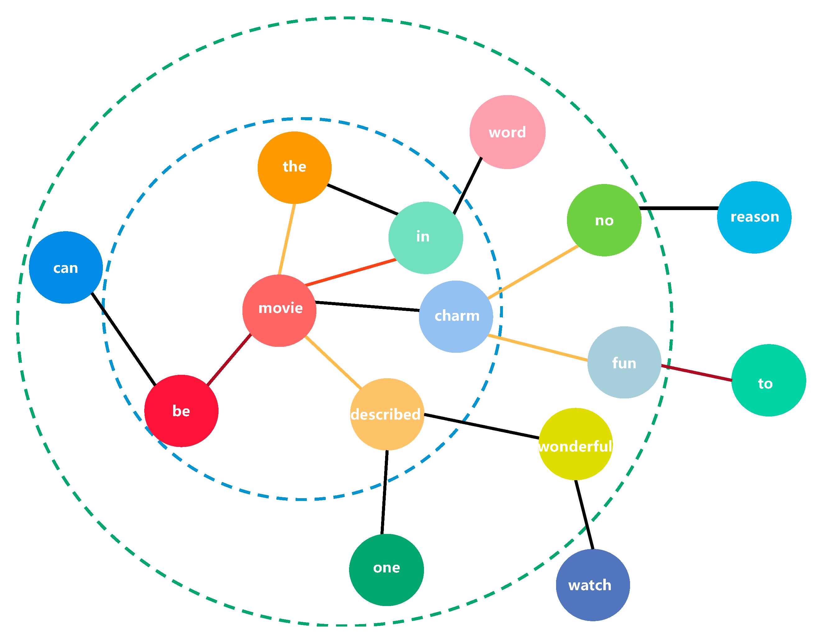
In addition, graph convolution based on word co-occurrence relationships and semantic dictionary composition can only capture the relationship of non-continuous entities in the text and cannot simultaneously capture the short-distance and long-distance dependencies of words in sentences. For example, a text graph is constructed from a corpus of word co-occurrence relations and semantic dictionaries, as shown in Figure 1. Here “This movie can be described in one word: wonderful.” is a sentence in the corpus. Taking “wonderful” as the center, the blue circle represents the aggregation of one-level neighbor node information, and the green circle represents the aggregation of two-level neighbor node information. Among them, “wonderful” is used to modify “movie” in the sentence, and it is very useful for analyzing the expression of the text as a whole. However, the two word nodes “movie” and “wonderful” in Figure 1 are not directly related, but there should be a certain dependency between them. Graph Convolutional Network only aggregates direct neighbor node information, so one layer of GCN can only capture short-distance dependencies of words in sentences. Capturing long-range dependencies between words such as “movie” and “wonderful” can be solved by increasing the number of GCN layers. However, current research shows that multi-layer graph convolutional networks for text classification tasks incur high space complexity. At the same time, increasing the number of network layers will also make the local features converge to similar values. To overcome this problem, we introduce dependencies when building the text graph. Dependency syntax is mainly concerned with the relationship between words (sentence components) in a sentence, and it is not affected by the physical location of the components. By introducing dependencies, short-range dependencies and long-range dependencies can be well utilized while also providing syntactic constraints and partially reducing the number of GCN layers.

However, due to the characteristics of the graphs, when learning word features, graph convolutional networks do not effectively capture the word order that is very useful for them, resulting in the loss of contextual semantic information of the text. For example, “You have a lot of hard work.”, “You have to work hard.”, where the word “work” will change meaning depending on its position in the contextual sentence. The graph formed by the words in these two sentences cannot reflect the order between the words, so it cannot represent the characteristics of word order changes. Obviously, this is very important for understanding the meaning of the sentence. In addition, the graph convolutional network cannot distinguish polysemy; for example, “She’s grown into quite an individual.”, “So this individual came up.”, the meaning of the word “individual” expresses different semantics depending on the context. In the first sentence, it is the meaning of “person with personality”, and in the second sentence, it has the meaning of “weird person”. In this case, if not differentiated, it may affect the understanding of the text, thereby affecting the classification effect. Leveraging multilayer multi-head self-attention and positional word embeddings, BERT mainly focuses on local contiguous word sequences that provide local contextual information. By pre-training a large amount of text data in different fields, BERT can well infer the meaning that polysemous words should express in the current context. However, BERT may have difficulty interpreting global information about vocabulary.

To improve the above-mentioned problems, this paper proposes an improved model (IMGCN) for text classification. On the basis of Vocabulary Graph Convolution (VGCN) [15], a semantic dictionary (WordNet) and dependencies are introduced, and the features of GCN and BERT are further learned through residual bi-layer BiLSTM with an attention mechanism [17]. By building dependencies, GCNs can be made to capture long-range dependencies of words in sentences more efficiently. WordNet was introduced to provide more useful connections between words. At the same time, the BERT model is used to extract the local feature information of a text. The global vocabulary information obtained by GCN is combined with the context information obtained by pre-trained BERT. Considering that the text has a hierarchical structure of word-sentence-document, in order to obtain more comprehensive text features, we use hierarchical BiLSTM to extract the combined features hierarchically to capture word, sentence, and document feature information, respectively. In the process of word-to-sentence feature extraction, the attention mechanism is used to generate sentence embeddings, which solves the problem that keyword features cannot be paid attention to in text classification. We changed the initialization method of the context vector in the attention mechanism and combined the bidirectional word hidden features as the initial value of the context vector to guide the learning of the attention mechanism. By introducing residual connections, the neural network degradation problem that occurs when stacking multi-layer network models can be alleviated, and the model can learn residuals to better obtain new features.

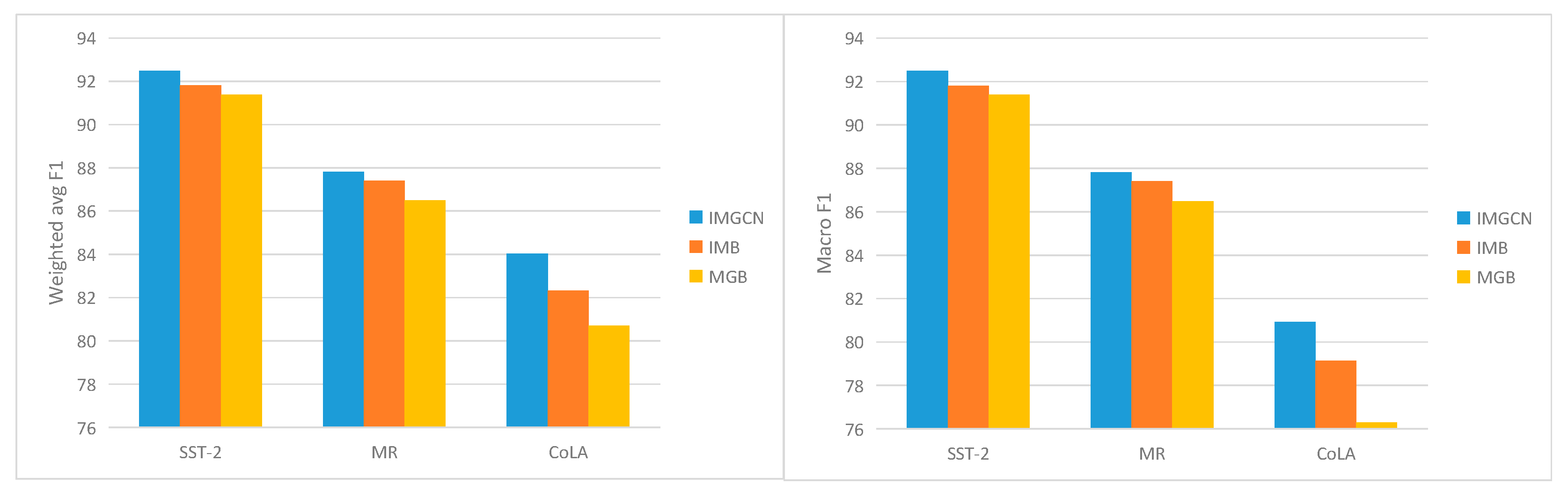
We call the proposed model IMGCN. Experiments on four benchmarking datasets demonstrate that IMGCN can effectively improve the results in current GCN-based methods and achieve better results. The main contributions of this paper are as follows:

• The dependency and semantic dictionary are fully integrated into IMGCN. They can enrich the connections between words and capture the long-range dependencies of words in sentences while providing syntactic constraints and partially reducing the number of GCN layers.
• Combining graph features and sequence features, using hierarchical BiLSTM to extract input features hierarchically, capturing word and sentence feature information, respectively, so as to obtain more comprehensive text features.

2. Related Work

Traditional text classification methods are mainly based on feature engineering. Feature engineering includes the bag-of-words model [18] and n-grams, etc. Later, there was research [19,20] that converted text into graphics and performed feature engineering on graphics. However, these methods cannot automatically learn the embedding representation of nodes. Compared with traditional methods, deep learning-based methods can automatically acquire features, and they can learn the deep semantic information of the text. In terms of deep learning models, Kim 2014 [3] uses a simple convolutional neural network (CNN) for text classification. Tang et al. 2015 [21] proposed a gated recurrent neural network. Yang et al. 2016 [17] proposed the use of hierarchical attention networks to model and classify documents. Wang et al. 2016 [22] introduced the attention mechanism into LSTM. Dong et al., 2020 [23] introduce the Bidirectional Encoder Representation from Transformers (BERT) [10] and the self-interaction attention mechanism. Most attention-based deep neural networks mainly focus on local continuous word sequences, which provide local context information. However, the ability to capture the global characteristics of the relevant information may not be sufficient.

In recent years, many studies have tried to apply convolution operations to graph data. Kipf and Welling 2017 [12] proposed Graph Convolutional Networks (GCNs), and the model has achieved good results on node classification tasks. Velickovic et al. 2018 [24] proposed a Graph Attention Network (GAT), which uses the attention mechanism [25] to assign weights to the neighborhood information of nodes. Compared with the GCN without adding weights, it has a better promotion. Later, Yao et al. 2019 [13] proposed the TextGCN model, which introduced the Graph Convolutional Network to text classification for the first time. By modeling the text into a graph, the nodes in the graph are composed of words and documents, and a good effect is finally obtained. Cavallari et al. 2019 [26] introduced a new setting for graph embedding, which considers embedding communities instead of individual nodes.

Now, many studies try to combine GCN with other models. Ye et al. 2020 [14] input the word and document nodes trained by GCN and BERT’s word vector into the BiLSTM classification model, where the input vector of GCN is a one-hot vector. Lu et al. 2020 [15] integrated the vocabulary graph embedding module with BERT and achieved good results in many public datasets, where GCN uses BERT’s word vector. In contrast to this, in our method, GCN uses BERT’s word vectors and uses dependencies when building the text graph. One graph focuses on extracting dependencies between words, and the other graph focuses on word co-occurrences. We use a two-layer BiLSTM with attention combined with GCN and BERT; one layer is used to focus on the word sequence, the other layer focuses on the sentence sequence, and a residual operation is added after BiLSTM to learn the residual.

3. Proposed Method

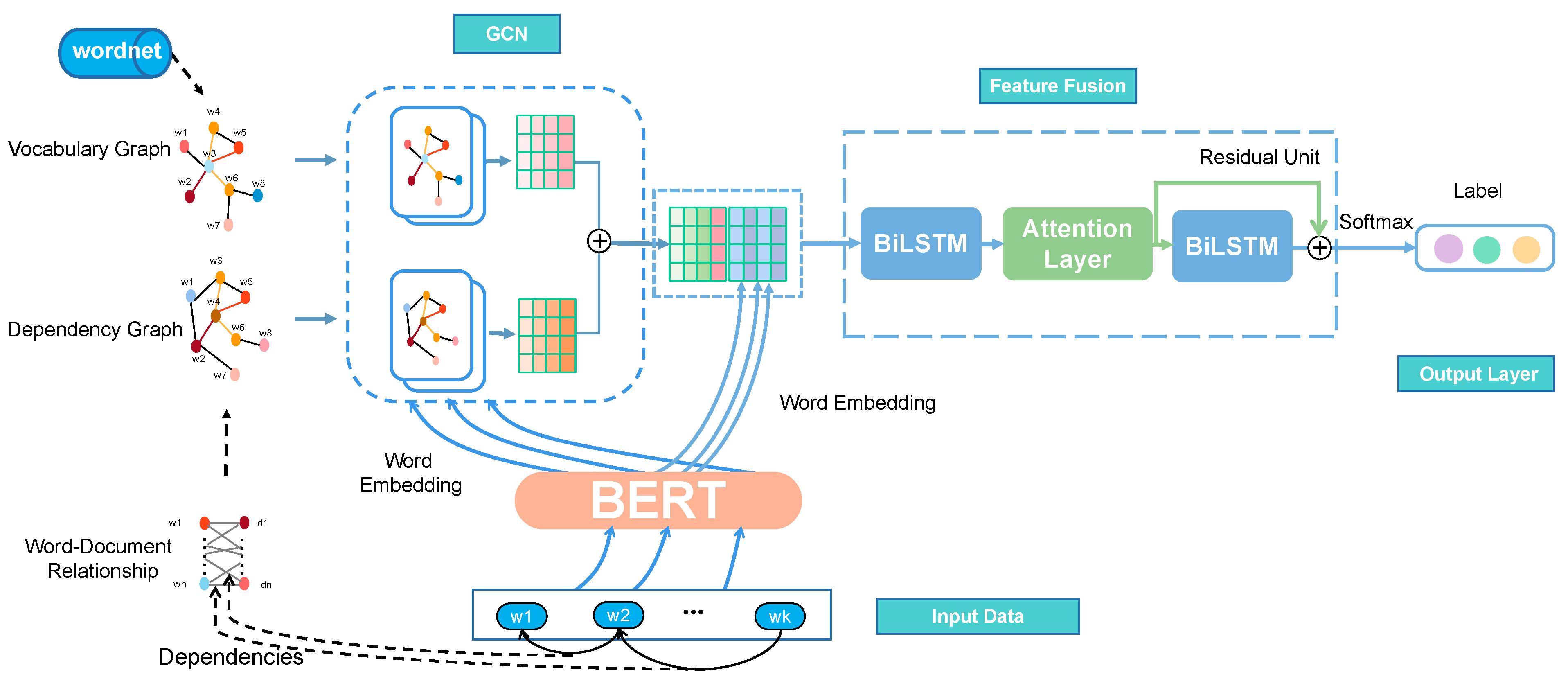
Following in-depth research on text classification based on neural networks, this paper proposes IMGCN. The whole process of IMGCN can be divided into the steps of text composition, graph convolutional network, feature fusion, and final prediction. The architecture of IMGCN is shown in Figure 2. The colored continuous line in the IMGCN architecture is the output of each single model, and the intermittent line represents the modules composed of a single model. We construct two text graphs by establishing edges between word nodes. Build a vocabulary graph from word co-occurrence relations and semantic lexicon. Build a dependency graph from the inclusion and dependencies of documents and words. We use point-wise mutual information (NPMI) [27] and a semantic dictionary to assign association weights to edges between words to jointly build a text graph. Then, the dependency-based TF-IDF method is used to assign association weights to the edges between words and documents and use a matrix transformation to map them to the relations between words and words, thereby constructing another text graph. Then the word embedding of BERT is used as the input vector required by the graph convolutional network, and the two text graphs are respectively used as the adjacency matrix required by the graph convolutional network. Subsequently, they are separately fed into a two-layer graph convolutional network for training, and the two hidden output vectors are then summed. Next, the added word vector is fused with the feature vector of the pre-trained BERT and input to the first-layer BiLSTM model to extract the semantic dependency information between words within a single sentence. To further distinguish the importance of words, we add an attention mechanism to the first layer of BiLSTM to distinguish the importance of words by assigning different word weights. The word weights and the output of the first layer of BiLSTM are weighted and summed to form an overall representation of the current sentence. Here, the bidirectional word hidden features are combined as the context vector of the attention mechanism to guide the learning of the attention mechanism. The obtained sentence feature representation is then input to the second layer of the BiLSTM to extract semantic dependency information between sentences within the text. The learned sentence feature representation and the feature obtained by the context attention layer are subjected to residual operation to form an overall text representation. Finally, the overall text representation is input to the Softmax classification layer to obtain the final category of the text.

3.1. Text Graph

3.1.1. Vocabulary Graph

In this paper, we first use a semantic dictionary (Wordnet) and Normalized Pointwise Mutual Information (NPMI) to construct a text graph. For constructing text graphs using word co-occurrence relationships, normalized pointwise mutual information (NPMI) is generally used to calculate edge weights between two word nodes, which is a common measure of word association. However, the calculation of NPMI depends on the corpus. If the probability of some words appearing in the corpus is low, this method may lead to a small calculation result of NPMI, and the similarity of two words is judged to be low or not. For example, the word “abundant” has a very low probability of appearing in the corpus. Let P (word and other words) be the co-occurrence probability between words. When calculating the co-occurrence probability of “abundant” and other words, the values of P (abundant and other words) and P (abundant) are very small; even if it is 0, it will result in a very small value of NPMI, so in the end, “abundant” and other words may be judged as having little or no semantic relevance.

In addition, there are a lot of connections between words, and the most direct connection is the synonymous relationship that exists between certain words. For example, the words “abundant” and “plentiful” have very similar meanings and can be used interchangeably in most cases. If two words are synonymous, then only constructing a text graph through word co-occurrence relationship may lack this part of word relationship information. If this synonymous relationship can be used, the relationship information of words can be enriched, thereby improving the accuracy of the calculation. The semantic dictionary describes the different semantic relations between words. Therefore, we jointly construct a text graph using word co-occurrence relations and semantic lexicon.

For the selection of the semantic dictionary, we use WordNet. WordNet describes a network of semantic relationships between words. For every content word in the language, it gives all possible word meanings. WordNet organizes words in a dictionary using semantic and lexical relations, where semantic relations represent the degree of association between the semantic items of two words. Nouns, verbs, adverbs, and adjectives are each organized into a network of synonyms, each set of synonyms representing a basic semantic concept, and these sets are also connected by various relationships. Since a word can have multiple meanings, it is necessary to compare the meanings between the two words. Therefore, we first use WordNet to expand synonyms and then use the WordNet-based Wup method to calculate the semantic similarity between words in the two synonym sets and calculate the average of all similarity scores. This value is the final similarity score of the two words. The larger the calculated value, the higher the semantic similarity between them. Among them, the “Wup” method [28] is a similarity measurement method based on the path structure proposed by Wu and Palmer. The similarity is calculated according to the similarity of the meaning of the words and the position of the synonym sets in the hypernym tree relative to each other.

Therefore, for two words i and j, we first calculate the edge weights between two words using the NPMI method. If the calculated NPMI value is small, the WordNet-based method is used for calculation, which can minimize the problems caused by the low frequency of some words in the corpus, and at the same time, add more word relationship information. Formally, the edge weight between node i and node j is defined as:

$${\mathrm{A}}_{\mathrm{ij}}=\{\begin{array}{ll}\hfill \mathrm{NPMI}(\mathrm{i},\mathrm{j})\hfill & \mathrm{i},\mathrm{j}\mathrm{are} \mathrm{words}, \mathrm{NPMI}(\mathrm{i},\mathrm{j})>0\\ \hfill \mathrm{WordSim}(\mathrm{i},\mathrm{j})\hfill & 0.5\le \mathrm{WordSim}(\mathrm{i},\mathrm{j})\le 1, \mathrm{NPMI}(\mathrm{i},\mathrm{j})<0\\ \hfill 1\hfill & \mathrm{i}=\mathrm{j}\\ \hfill 0\hfill & \mathrm{otherwise}\end{array}$$

(1)

The NPMI value of a pair of words i, j is calculated as:

$$\mathrm{NPMI}(\mathrm{i},\mathrm{j})=-\frac{1}{\mathrm{logp}(\mathrm{i},\mathrm{j})}\log \frac{\mathrm{p}(\mathrm{i},\mathrm{j})}{\mathrm{p}\left(\mathrm{i}\right)\mathrm{p}\left(\mathrm{j}\right)}$$

(2)

where $\mathrm{p}\left(\mathrm{i},\mathrm{j}\right)=\frac{\#\mathrm{w}(\mathrm{i},\mathrm{j})}{\#\mathrm{w}}$, $\mathrm{p}\left(\mathrm{i}\right)=\frac{\#\mathrm{w}\left(\mathrm{i}\right)}{\#\mathrm{w}}$, $\#\mathrm{W}\left(\mathrm{i}\right)$ is the number of all sliding windows containing word i, $\#\mathrm{W}(\mathrm{i},\mathrm{j})$ is the number of all sliding windows containing word i and word j, and $\#\mathrm{W}$ is the total number of sliding windows. We set the window larger to gain long-term dependence. The value range of NPMI is $[-1, 1]$. A positive NPMI value indicates that the semantic relevance between words is high, while a negative NPMI value indicates that there is little or no semantic relevance. Therefore, we only create an edge between word pairs with positive NPMI values.

When the NPMI value of a pair of words i, j is calculated to be negative, their semantic similarity is calculated as:

$$\mathrm{WordSim}(\mathrm{i},\mathrm{j})=\frac{{{\displaystyle \sum }}_{\mathrm{q}=1}^{{\mathrm{len}}_2}{{\displaystyle \sum }}_{\mathrm{p}=1}^{{\mathrm{len}}_1}{\mathrm{sim}}_{\mathrm{wup}}\left({\mathrm{w}}_{\mathrm{p}},{\mathrm{k}}_{\mathrm{q}}\right)}{{\mathrm{len}}_1+{\mathrm{len}}_2-\mathrm{a}}$$

(3)

where ${\mathrm{sim}}_{\mathrm{wup}}{(\mathrm{w}}_{\mathrm{p}}{,\mathrm{k}}_{\mathrm{q}})=\frac{{2\times \mathrm{N}}_3}{{\mathrm{N}}_1{+\mathrm{N}}_2{+2\times \mathrm{N}}_3}$ represents the semantic similarity of two words in the synonym lexicon, Let ${\mathrm{s}}_3$ be the deepest parent concept of ${\mathrm{w}}_{\mathrm{p}}$ and ${\mathrm{k}}_{\mathrm{q}}$, ${\mathrm{N}}_1$ is the number of nodes on the path from ${\mathrm{w}}_{\mathrm{p}}$ to ${\mathrm{s}}_3$, ${\mathrm{N}}_2$ is the number of nodes on the path from ${\mathrm{k}}_{\mathrm{q}}$ to ${\mathrm{s}}_3$, and ${\mathrm{N}}_3$ is the root of the concept hierarchy tree from ${\mathrm{s}}_3$ the number of nodes on the path of the node. Let ${\mathrm{S}}_1=\left\{{\mathrm{w}}_1{,\mathrm{w}}_2, \dots {, \mathrm{w}}_{\mathrm{p}}\right\}, \mathrm{p} \in \left[{1, \mathrm{len}}_1\right]$ be the synonym word set of word i, ${\mathrm{len}}_1$ be the number of words in ${\mathrm{S}}_1$, ${\mathrm{S}}_2=\left\{{\mathrm{k}}_1{,\mathrm{k}}_2, \dots {, \mathrm{k}}_{\mathrm{q}}\right\}, \mathrm{q} \in \left[{1, \mathrm{len}}_2\right]$ be the synonym word set of word j, ${\mathrm{len}}_2$ be the number of words in ${\mathrm{S}}_2$, and a is the number of word pairs with 0 semantic similarity in the word set. The value range of $\mathrm{WordSim}(\mathrm{i},\mathrm{j})$ is $[0, 1]$. If the $\mathrm{WordSim}(\mathrm{i},\mathrm{j})$ values of the two words are within a certain range, we create an edge between the two words. Experiments show that the performance is better when $\mathrm{WordSim}(\mathrm{i},\mathrm{j})$ is between 0.5 and 1.

3.1.2. Dependency Graph

Based on the above two relational compositions, graph convolutional networks can capture short-range dependencies of words in sentences but cannot capture long-range dependencies at the same time. Therefore, we introduce dependencies to construct another text graph to overcome the above problems. In addition, in order to obtain the inclusion relationship between documents and words while introducing the dependencies between words, we combine the two relationships. The edge weights between general document nodes and word nodes are calculated using the TF-IDF algorithm. TF-IDF is the word frequency-inverse text frequency index. The term frequency (TF) is the number of times a word appears in the document, and the inverse text frequency (IDF) reflects the general importance of the feature word in the corpus. However, the TF-IDF method lacks the combination of textual semantics, which is useful for understanding textual content. To overcome this problem, we refer to [29], introduce dependencies, and use an improved edge weight calculation method to understand and optimize text features.

Dependency syntax is mainly concerned with the relationship between the various words in a sentence, and it is not affected by the physical location of the components [30]. Since the importance and relevance of various dependencies in a sentence are not the same, first, the importance of words to sentences, texts, and even categories is determined according to the different dependencies between words and predicates in terms of word meaning. Then, according to the importance of different components to the sentence, the sentence composition is divided into eight levels.

The results of dependency analysis are usually represented by a labeled directed graph. For example, as shown in Figure 3, “root” represents the central word “has”. Examples of the relationship between the performance head word and its subsidiary words are “has” and “performances”. The result of dependency analysis shows that the relationship between these two words is a direct object (dobj, direct object) relationship.

After classifying the text features in the data set according to the dependency relationship, this paper uses the following dependency-based TFIDF weight calculation method [29]. The specific steps are as follows:

For the word i, we calculate the number of times that the word i appears in the text and set it as n. Then, according to the result of the dependency syntax analysis implemented by Stanford Parser, it is obtained that the word i belongs to the m-th $(1 \le \mathrm{m} \le \mathrm{n})$ sentence component in the text. Furthermore, according to paper [29], classify the m-th occurrence of word i in the text into ${\mathrm{k}}_{\mathrm{i},\mathrm{m}}$ level, and assign weight ${\mathrm{w}}_{\mathrm{i},\mathrm{m}}$ to it. The calculation process is shown in Formula (4):

$${\mathrm{w}}_{\mathrm{i},\mathrm{m}}=2\cos [(\frac{{\mathrm{k}}_{\mathrm{i},\mathrm{m}}}{8}{)}^{\mathsf{\lambda }}\times \frac{\mathsf{\pi }}{2}]$$

(4)

$${\mathrm{TF}}_{\mathrm{i}}={{\displaystyle \sum }}_{\mathrm{m}=1}^{\mathrm{n}}{\mathrm{w}}_{\mathrm{i},\mathrm{m}}$$

(5)

$${\mathrm{TF}\text{-}\mathrm{IDF}}_{\mathrm{i}}=\frac{{\mathrm{TF}}_{\mathrm{i}}}{\mathrm{s}} \times \log (\frac{\mathrm{D}}{{\mathrm{p}}_{\mathrm{i}}}+0.01)$$

(6)

Then the improved frequency ${\mathrm{TF}}_{\mathrm{i}}$ with the weight of word i in the text is calculated by Formula (5). For word i, the improved ${\mathrm{TFIDF}}_{\mathrm{i}}$ weight based on the dependency relationship is as shown in Formula (6). Where s represents the total number of words in the text where the word i is located, pi represents the number of texts containing the word i, and D represents the total number of texts in the dataset. Where λ is a parameter, which is used to adjust the weight gap between feature levels, and the range is [0,1].

Calculate the weight of the edge between the word node and the document node according to the above method, and obtain the adjacency matrix A, as shown in Formula (7). Then, the relationship between the words and documents is mapped to the relationship between words and words containing document information and dependencies through matrix transformation so as to construct another text graph $\stackrel{\sim }{\mathrm{A}}$.

$$\stackrel{\sim }{\mathrm{A}}={\mathrm{A}}^{\mathrm{T}}\mathrm{A}$$

(7)

where $\mathrm{A}\in {\mathrm{R}}^{\mathrm{n}\times \mathrm{m}}{}_{ }$, n is the number of document nodes and m is the number of word nodes.

3.2. Vocabulary GCN

A general graph convolutional network is a multi-layer (usually two-layer) neural network that performs convolution directly on the graph and updates a node’s embedding vector based on the information of its neighbor nodes. The graph nodes of a graph convolutional network are “task entities”, such as documents that need to be classified. It requires all entities, including those from training, validation, and test sets, to be displayed in the graph, so that node representations are not missing from downstream tasks. This limits the application of graph convolutional networks to many prediction tasks where test data are not seen during training. Therefore, we use Vocabulary Graph Convolution (VGCN), whose graph is constructed on the vocabulary without using the training set to obtain entities, mainly convolving related words. Then for a single document, the single-layer graph convolution is shown in Formula (8):

$$\mathrm{H}=\mathrm{X}\stackrel{\sim }{\mathrm{A}}\mathrm{W}$$

(8)

where $\stackrel{\sim }{\mathrm{A}}$ represents the vocabulary graph. $\mathrm{X}\stackrel{\sim }{\mathrm{A}}$ to extract part of vocabulary related to the input matrix $\mathrm{X}$, combining the words in the input sentence with the relevant words in the vocabulary. W hold hidden state vector of a weight of a single document, dimension is $\left|\mathrm{V}\right| \times \mathrm{h}$.

The corresponding two-level GCN with LeakyReLU function is:

$$\mathrm{GCN}=\mathrm{LeakyReLU}\left({\mathrm{X}}_{\mathrm{mv}}{\stackrel{\sim }{\mathrm{A}}}_{\mathrm{vv}}{\mathrm{W}}_{\mathrm{vh}}\right){\mathrm{W}}_{\mathrm{hc}}$$

(9)

where m is the mini-batch size, v is the vocabulary size, h is the hidden layer size, and c is the class size or sentence embedding size. W holds the weight of the hidden state vector of a single document. Each row of ${\mathrm{X}}_{\mathrm{mv}}$ is a vector containing document features, which is the word embedding of BERT. Then a two-layer convolution is performed to combine the words in the input sentence with the related words in the vocabulary.

Specifically, we perform two layers of graph convolution for the two text graphs generated in the previous section, then add the two generated hidden layer vectors.

In the training process of the original GCN, ReLU is used as the activation function of the GCN. In this paper, the non-linear function LeakyReLU is selected as the activation function of GCN, which overcomes the problem of gradient disappearance and speeds up training. In addition, L2 regularization is also used to reduce overfitting. The LeakyReLU function is as follows:

$$\mathrm{LeakyReLU}\left(\mathrm{x}\right)=\{\begin{array}{ll}0.2\mathrm{x},& \mathrm{x} < 0\\ \mathrm{x},& \mathrm{x} \ge 0\end{array}$$

(10)

3.3. Feature Fusion and Classification

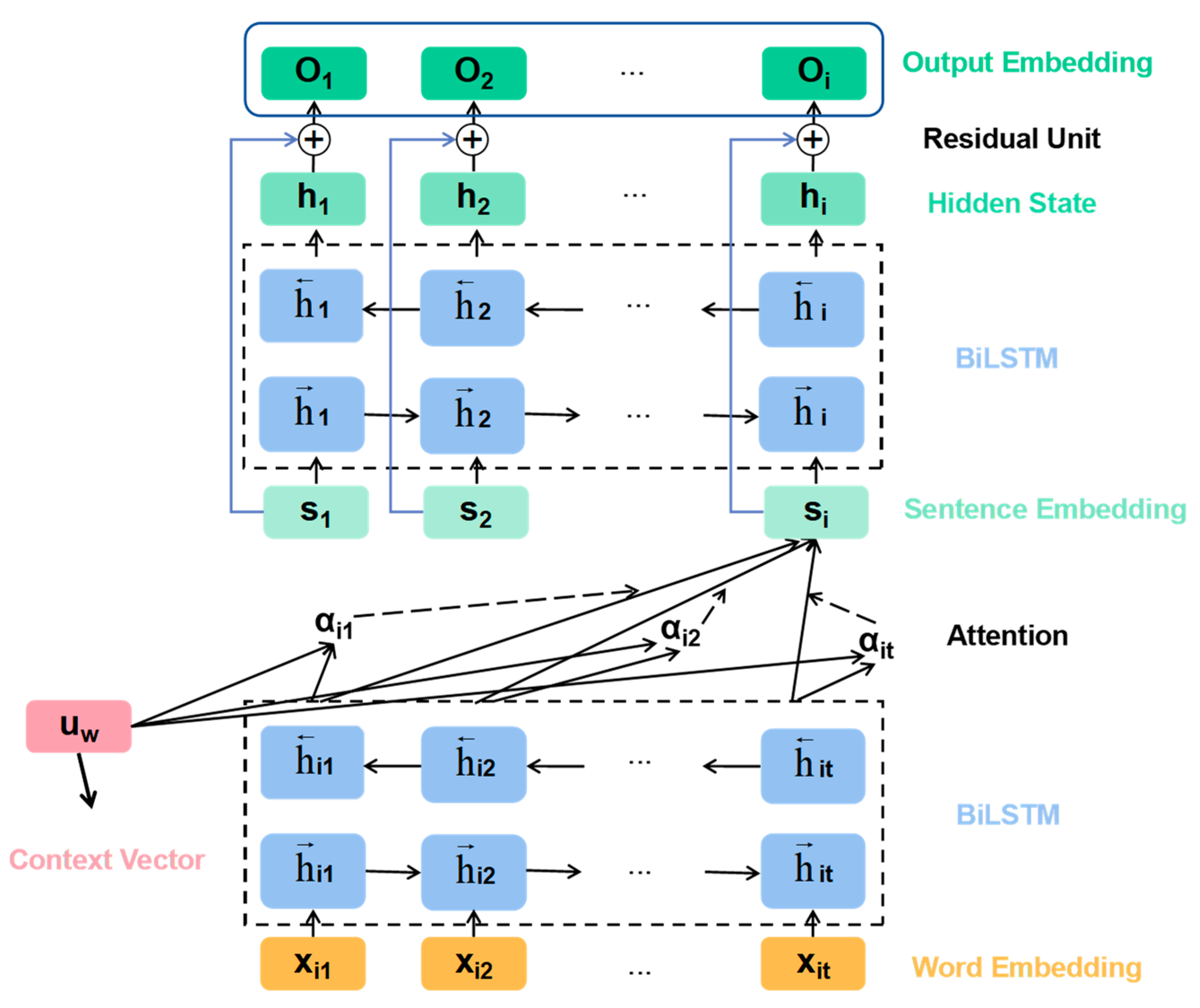
Since words are represented as nodes, the neighborhood information of nodes is aggregated through an adjacency matrix, ignoring the order structure of a text, resulting in the loss of contextual semantic information of a text. Therefore, we combine the global vocabulary information obtained by GCN with the context information obtained by the pre-trained BERT. While using the global vocabulary information, we can also take into account the order of words to capture contextual information. In order to dig deeper into the semantics, the sequence model LSTM can be used to fuse the two parts of information, but it can only capture features in a single direction, from front to back or from back to front. The mode of human reading text is to use the foregoing and the following to jointly infer the meaning of a word when encountering a word. Therefore, BiLSTM models that can capture features in both front-to-back and back-to-front directions are more in line with this pattern. Considering that text has a hierarchical structure, the text is composed of sentences, and sentences are composed of words. Therefore, we use a two-layer BiLSTM to learn word features and sentence features, respectively. Since the feature words have different importance to the text, and the output vector of BiLSTM does not distinguish the importance of words, we add an attention mechanism to its hidden output. We changed the initialization method of the context vector in the attention mechanism and combined the bidirectional word hidden features as the initial value of the context vector to guide the learning of the attention mechanism. At the same time, in order to prevent the deepening of the model layers from affecting the classification results, we introduced the residual operation. The specific structure of the model feature fusion module is shown in Figure 4.

The module consists of a semantic feature splicing layer, word-level feature extraction layer, contextual attention layer, and a sentence-level feature extraction layer. First, the GCN and the pre-trained BERT model convert the text word sequence into two different word vector representations. Secondly, the corresponding fusion of the obtained two different word vector representations is input into the first-layer BiLSTM model to extract the semantic dependency information between words within a single sentence, and a layer of attention mechanism is added to the first-layer BiLSTM, constructs an overall representation of the current sentence. Here, the bidirectional word hidden features are combined as the context vector of the attention mechanism. Then the obtained sentence feature representation is input to the second layer BiLSTM to extract semantic dependency information between sentences within the text. The learned sentence feature representation and the sentence feature representation obtained by the context attention layer are subjected to residual operation to form an overall text representation. Finally, the overall text representation is input to the Softmax classification layer to obtain the final category of the text.

3.3.1. Semantic Feature Connection Layer

We do not directly classify the output features of GCN but use the generated hidden feature representation ${\mathrm{H}}^{\left(2\right)}$ for subsequent learning. Since ${\mathrm{H}}^{\left(2\right)}$ does not adequately capture contextual information and does not discriminate word vector representations of polysemy, pre-trained BERT is introduced. The BERT model uses a bidirectional transformer structure for encoding, which can characterize the specific semantics of each word in the context and distinguish multiple semantics according to the semantic relationship of the context. Each word obtains the word vector representation W of the text through the pre-trained BERT model, as shown in Formula (11):

$${\mathrm{W}}^{\left(\mathrm{i}\right)}=\left\{{ \mathrm{w}}_1^{\left(\mathrm{i}\right)}{,\mathrm{w}}_2^{\left(\mathrm{i}\right)}, \dots {, \mathrm{w}}_{\mathrm{j}}^{\left(\mathrm{i}\right)}, \dots { \mathrm{w}}_{\mathrm{n}}^{\left(\mathrm{i}\right)}\right\}$$

(11)

where ${\mathrm{W}}^{\left(\mathrm{i}\right)}$ represents the vector matrix of the i-th text, ${\mathrm{w}}_{\mathrm{j}}^{\left(\mathrm{i}\right)}$ represents the feature vector of the j-th word in the i-th text, and n represents the maximum sentence length.

Then, the embedded representation ${\mathrm{H}}^{\left(2\right)}$ output after the second layer graph convolution operation in the GCN model is spliced with the word vector W generated by the pre-trained BERT to obtain a multi-feature vector X, as shown in Formula (12):

$$\mathrm{X}=\mathrm{concat}(\mathrm{W},{\mathrm{H}}^{\left(2\right)})$$

(12)

3.3.2. Word-Level Feature Extraction Layer

After the semantic feature connection layer is the word-level feature layer BiLSTM model, which is used to extract semantic dependency information between words within a single sentence. The BiLSTM model corresponds to the forward and backward LSTM models. The sequence information and contextual features are captured by LSTMs in two directions, and the combination of the two output layers generated by the two directions can provide past contextual information and future contextual information. The input of this layer of BiLSTM is the result X after semantic feature concatenation.

Suppose a text has L sentences ${\mathrm{s}}_{\mathrm{i}}$, where $\mathrm{i} \in \left[1,\mathrm{L}\right]$, and each sentence contains ${\mathrm{T}}_{\mathrm{i}}$ words. ${\mathrm{x}}_{\mathrm{it}}^{ }$ represents the word vector of the t-th word in the i-th sentence, where $\mathrm{t} \in \left[1,\mathrm{T}\right]$. In the forward LSTM layer, read sentence s ${\mathrm{s}}_{\mathrm{i}}$ from ${\mathrm{x}}_{\mathrm{i}1}^{ }$x to ${\mathrm{x}}_{\mathrm{it}}^{ }$y and perform forward calculation to obtain the hidden state $\overrightarrow{{\mathrm{h}}_{\mathrm{it}}^{ }}$h; in the backward LSTM layer, read sentence ${\mathrm{s}}_{\mathrm{i}}$s from ${\mathrm{x}}_{\mathrm{it}}^{ }$y to ${\mathrm{x}}_{\mathrm{i}1}^{ }$x and perform reverse calculation to obtain the hidden state $\overleftarrow{{\mathrm{h}}_{\mathrm{it}}^{ }}$m, as shown in Equations (13) and (14):

$$\overrightarrow{{\mathrm{h}}_{\mathrm{it}}^{ }}=\overrightarrow{{\mathrm{LSTM}}_{ }^{ }}{(\mathrm{x}}_{\mathrm{it}}^{ },\overrightarrow{{\mathrm{h}}_{\mathrm{it}-1}^{ }}), \mathrm{t} \in \left[1,\mathrm{T}\right]$$

(13)

$$\overleftarrow{{\mathrm{h}}_{\mathrm{it}}^{ }}=\overleftarrow{{\mathrm{LSTM}}_{ }^{ }}{(\mathrm{x}}_{\mathrm{i}}^{ },\overleftarrow{{\mathrm{h}}_{\mathrm{it}-1}^{ }}), \mathrm{t} \in \left[\mathrm{T},1\right]$$

(14)

Finally, the hidden state $\overrightarrow{{\mathrm{h}}_{\mathrm{it}}^{ }}$ obtained by the forward LSTM layer is spliced with the hidden state $\overleftarrow{{\mathrm{h}}_{\mathrm{it}}^{ }}$ obtained by the backward LSTM layer to obtain the final hidden layer state ${\mathrm{h}}_{\mathrm{it}}^{ }$ of the bidirectional LSTM, as shown in Formula (15):

$${\mathrm{h}}_{\mathrm{it}}^{ }=\left[\overrightarrow{{\mathrm{h}}_{\mathrm{it}}^{ }},\overleftarrow{{\mathrm{h}}_{\mathrm{it}}^{ }}\right]$$

(15)

3.3.3. Contextual Attention Layer

Considering that the words in a sentence contribute differently to the meaning expression of the sentence, the attention mechanism can focus on important information from a large amount of information while ignoring unimportant information. Therefore, an improved attention mechanism is used to focus on important information, and these word representations are aggregated to form sentence feature representations. The hidden output result ${\mathrm{h}}_{\mathrm{it}}^{ }$ of the word-level feature layer is used as the input of the context attention layer, and the calculation process of assigning attention weights is shown in Equations (16) and (17):

$${\mathrm{u}}_{\mathrm{it}}^{ }{=\tan \mathrm{h}(\mathrm{W}}_{\mathrm{w}}{\mathrm{h}}_{\mathrm{it}}^{ }{+\mathrm{b}}_{\mathrm{w}})$$

(16)

$${\mathsf{\alpha }}_{\mathrm{it}}^{ }=\frac{{\exp (\mathrm{u}}_{\mathrm{it}}^{ }{}^{\mathrm{T}}{\mathrm{u}}_{\mathrm{w}})}{{\sum }_{\mathrm{t}}\exp \left({\mathrm{u}}_{\mathrm{it}}^{\mathrm{T}}{\mathrm{u}}_{\mathrm{w}}\right)}$$

(17)

where ${\mathrm{W}}_{\mathrm{w}}$ is the weight matrix, ${\mathrm{b}}_{\mathrm{w}}$ is the bias term, and ${\mathsf{\alpha }}_{\mathrm{it}}^{ }$ is the normalized importance weight. ${\mathrm{u}}_{\mathrm{w}}$ is the attention context vector, which contains useful information for the text to guide the attention model to locate informative words from the input sequence, and thus plays an important role in the attention mechanism. Prior work either ignores the context vector or initializes it randomly, which greatly weakens the role of context. Therefore, we use the combination of word hidden features learned by LSTM in two directions as the context vector of the attention mechanism, that is, ${\mathrm{u}}_{\mathrm{w}}{=\mathrm{h}}_{\mathrm{it}}^{ }{+\mathrm{h}}_{\mathrm{i}1}^{ }$. It contains contextual information of words in sentences to guide the learning of the attention mechanism.

Next, the word importance weight calculated by Formula (17) and the hidden output result ${\mathrm{h}}_{\mathrm{it}}^{ }$ of the word-level feature layer are weighted and summed. The word-level feature vectors are aggregated into sentence-level feature vectors ${\mathrm{s}}_{\mathrm{i}}$ to form an overall representation of the current sentence, as shown in Formula (18):

$${\mathrm{s}}_{\mathrm{i}}={\displaystyle {\sum }_{\mathrm{t}}}\left({\mathsf{\alpha }}_{\mathrm{it}}^{ }{\mathrm{h}}_{\mathrm{it}}^{ }\right)$$

(18)

3.3.4. Sentence Level Feature Extraction Layer

Since a text contains multiple sentences, there are semantic dependencies between each sentence. Therefore, the main task of the sentence-level feature extraction layer is to extract the semantic dependency information between sentences within the text in units of sentences. The sentence vector ${\mathrm{s}}_{\mathrm{i}}$ obtained by the contextual attention layer is input into a layer of BiLSTM for sentence sequence learning. Where $\overrightarrow{{\mathrm{h}}_{\mathrm{l}}^{ }}$ is the hidden state obtained by the forward LSTM layer through the forward input, $\overleftarrow{{\mathrm{h}}_{\mathrm{l}}^{ }}$ is the hidden state obtained by the backward LSTM layer through the reverse input, and finally, the two hidden states are spliced to obtain ${\mathrm{h}}_{\mathrm{i}}^{ }$.

$$\overrightarrow{{\mathrm{h}}_{\mathrm{l}}^{ }}=\overrightarrow{{\mathrm{LSTM}}_{ }^{ }}{(\mathrm{s}}_{\mathrm{i}}^{ },\overrightarrow{{\mathrm{h}}_{\mathrm{t}-1}^{ }}), \mathrm{t} \in \left[1,\mathrm{L}\right]$$

(19)

$$\overleftarrow{{\mathrm{h}}_{\mathrm{l}}^{ }}=\overleftarrow{{\mathrm{LSTM}}_{ }^{ }}{(\mathrm{s}}_{\mathrm{i}}^{ },\overleftarrow{{\mathrm{h}}_{\mathrm{t}-1}^{ }}), \mathrm{t} \in \left[\mathrm{L},1\right]$$

(20)

$${\mathrm{h}}_{\mathrm{i}}^{ }=\left[\overrightarrow{{\mathrm{h}}_{\mathrm{l}}^{ }},\overleftarrow{{\mathrm{h}}_{\mathrm{l}}^{ }}\right]$$

(21)

The deepening of the number of network layers can improve the accuracy of the model, but there are problems with the disappearance of the gradient of the deep network and the degradation of the network. When the depth reaches a certain level, the accuracy of the model begins to decline again, and the fitting ability becomes worse. In the deep neural network, the residual network can effectively inhibit the network degradation phenomenon and avoid the problem of sub-optimal solutions in deeper networks. Therefore, we introduce a residual connection between two adjacent layers and perform a residual operation on the sentence feature representation learned by the sentence-level feature extraction layer and the sentence feature representation output by the context attention layer. Let the model learn the residual to obtain a higher-level feature representation to achieve a better classification effect, as shown in Formula (22):

$${\mathrm{O}}_{\mathrm{i}}{=\mathrm{s}}_{\mathrm{i}}^{ }{+\mathrm{h}}_{\mathrm{i}}^{ }$$

(22)

Finally, the result ${\mathrm{O}}_{\mathrm{i}}$ is input to the Softmax layer for classification, and the final category of the text can be obtained.

4. Discussion

In this section, we will conduct experiments on four publicly available datasets and analyze the experimental results of different models. Subsequently, ablation studies were performed to further explore the effectiveness of each component.

4.1. Datasets

For an overall comparison with other more advanced methods, we choose the SST-2 dataset [31], MR [32], CoLA [33], and R8 dataset [13], which are commonly used in other methods to evaluate our proposed method. The four datasets contain the content of reviews, grammar, and news. The SST-2 dataset is the Stanford Sentiment Treebank dataset, which is a binary single-sentence classification task consisting of sentences extracted from movie reviews and human annotations of their sentiments. We use the public version, which has 6920 training samples, 872 validation samples, and 1821 test samples. In total, there are 4963 positive reviews and 4650 negative reviews. The average length of reviews is 19.3 words. The MR dataset is a sentiment classification dataset for movie reviews. We used the public version in [34] with 3554 test samples, 6392 training samples, and 710 validation samples. The average length of reviews is 21.0 words. The CoLA dataset is a grammar dataset released by New York University. This task is mainly to judge whether the grammar of a given sentence is correct, which belongs to the single-sentence text binary classification task. We use the public version with 8551 training data, 1043 validation data, and 1062 test samples for a total of 6744 positives and 2850 negatives. The average length is 7.7 words. The R8 dataset represents a subset of the Reuters 21,578 dataset. The dataset includes eight categories, divided into 5485 training documents and 2189 test documents. We randomly select 20% of the training set of this dataset as the validation set. The average length is 65.72 words.

4.2. Implementation Details

The WordNet threshold of all datasets in this paper is set to 0.5. When calculating NPMI on the dataset, the entire sentence is used as a text window to construct a vocabulary graph. The NPMI threshold of all datasets is set to 0.2 to filter out meaningless relationships between words. In the IMGCN model, the graph embedding output size is set to 16, and the hidden dimension of graph embedding is set to 128. We use the pre-trained BERT model provided by Google and set the maximum sequence length to 200. The dropout rate is set to 0.2. We train the model in 15 epochs. The batch size is set to 16. The Learning rate of the SST-2 dataset is set to 1 × 10⁻⁵, and the Learning rate of the other datasets is set to 8 × 10⁻⁵. The loss weight decay of the CoLA dataset is set to 0.0001, and the loss weight decay of other datasets is set to 0.001.

4.3. Main Experimental Results

To verify the performance of the proposed model, we conduct comparative experiments with other models. Including the classic Bi-LSTM [35], Text-GCN [13], and BERT [10] models, and three improved GCN methods: VGCN [15], VGCN-BERT [15], and STGCN + BERT + BiLSTM [14].

• Bi-LSTM: Bidirectional LSTM is often used for text classification. Use BERT pre-trained word embeddings as input to the Bi-LSTM model.
• Text-GCN: A text classification method that uses graphs to model text. The words and documents in the text are regarded as nodes, where the edges of the document and the words are based on the appearance information of the words in the document, and the edges of the words and the words are based on the global word co-occurrence information of the words. It has many improvements over many of the most advanced models.
• VGCN: The model only uses VGCN. The pre-trained word embedding of BERT is used as an input. The output of VGCN is relayed to a fully connected layer with the Softmax function to generate classification scores. This model only uses the global information of the vocabulary graph.
• BERT: We use a small version (BERT-base-uncase) of pre-trained BERT.
• VGCN-BERT: Based on the word co-occurrence information, a graph convolutional network is constructed on the vocabulary graph, and then the graph embedding and word embedding are provided to the self-attention encoder in BERT.
• STGCN + BERT + BiLSTM: The topic model is employed to extract the short text topic information, and a short-text graph is constructed by word co-occurrence and document word relations. The word nodes and document nodes trained by the GCN and vectors generated by the BERT’s hidden layer are fed together to the BiLSTM classifier for short text classification.

In order to comprehensively evaluate the model, the weighted average F1-Score and macro F1-Score are selected as evaluation indicators. The main results on the accuracy, weighted average F1-Score, and macro F1-Score on test sets are presented in

Table 1. Accuracy, Weighted average F1-Score and (Macro F1-score) on the test sets.

Model	SST-2		MR		CoLA		R8
	Weighted Avg F1 (Macro F1)	Acc	Weighted Avg F1 (Macro F1)	Acc	Weighted Avg F1 (Macro F1)	Acc	Weighted Avg F1 (Macro F1)	Acc
Text-GCN	80.45	82.39	75.67	76.70	56.18 (52.30)	52.30	—	97.00
Bi-LSTM	81.32	83.50	76.39	77.70	62.88 (55.25)	64.10	—	96.30
VGCN	81.64	83.43	76.42	76.42	63.59 (54.82)	65.61	97.12 (94.65)	97.43
BERT	91.49	91.53	86.24	80.30	81.22 (77.02)	81.20	98.12 (95.59)	98.20
STGCN + BERT + BiLSTM	—	—	—	82.50	—	—	—	98.50
VGCN-BERT	91.93	91.94	86.35	86.35	83.68 (80.46)	83.70	98.04 (95.43)	98.04
IMGCN	92.48	92.48	87.81	87.81	84.02 (80.91)	84.37	98.14 (96.50)	98.34

. The experimental results on four benchmark datasets confirm that the performance of IMGCN is basically better than other baseline models, which further proves the effectiveness and robustness of IMGCN in text classification. The “—” in the table represents no data. The bold in the table indicates the best results of the model. The Macro F1 score is the arithmetic average of multiple F1 scores, and it assigns equal weight to each class. The weighted avg F1 score assigns different weights to different classes according to the number of samples in each class. When calculating the two scores, the respective Macro F1 scores and Weighted avg F1 scores of the SST-2 and MR datasets are close. Since we rounded our calculations to two decimal places, this resulted in the macro F1 score and the weighted average F1 score being the same on SST-2 and MR.

It can be seen from the table that IMGCN has a good classification effect compared with the baseline models, which proves the effectiveness of the model in this paper. The performance of the Bi-LSTM model and the models VGCN and Text-GCN that utilize the vocabulary graph are comparable. Compared with the VGCN and BERT models, the model in this paper has a certain degree of effect improvement, indicating that the introduction of dependencies, semantic dictionaries, the BERT model, Bi-LSTM model, and residual attention in this model does enrich the contextual semantic information and local feature information of GCN, making the model in this paper compared to other models have better classification performance. At the same time, compared with VGCN-BERT, IMGCN always performs better. All this shows that the combination of each component of this paper is useful.

4.4. Ablation Study

In order to further study the benefits of the various components of IMGCN, this paper conducted ablation experiments on the effectiveness of the constructed model. Since the experimental results of IMGCN and the three variant models on the R8 dataset are not much different,

Table 2. Experimental results of ablation study.

Model	SST-2		MR		CoLA
	Weighted Avg F1	Macro F1	Weighted Avg F1	Macro F1	Weighted Avg F1	Macro F1
MGB	91.38	91.38	86.49	86.49	80.70	76.30
IMB	91.80	91.80	87.40	87.40	82.32	79.12
IMGCN	92.48	92.48	87.81	87.81	84.02	80.91

only shows the results of the ablation experiments on the three public datasets of SST-2, MR, and CoLA. We selected two indicators, weighted average F1-Score and macro F1-Score. The experimental results of the IMGCN and the three variant models prove that the three components used in this paper can improve the performance of IMGCN. Among them, MGB is a model that only uses point-state mutual information to build a graph network for learning and stitches it together with the local information obtained by BERT. Based on the MGB model, IMB introduces a model that relies on syntactic and semantic dictionaries for composition. IMGCN is a model that further fuses graph features and local features obtained by BERT using hierarchical BiLSTM on the basis of IMB.

As shown in Table 2, we can see that the performance of the model with the corresponding module added has a certain degree of improvement compared with the overall model, indicating that the modules are complementary to each other. It can be observed that different modules have different functions in different datasets.

As shown in Figure 5, the performance of the model named IMB has a certain improvement compared to the MGB model. The F1 score of the IMB model on the three datasets is higher than that of the IGB model. Although the gap is not high, it also proves that the introduction of dependency syntax and semantic dictionary can enrich the word embedding information of the graph. Compared with the F1 score of the IMB model, the F1 scores of the SST-2, MR, and CoLA datasets on the IMGCN model all increased to varying degrees. This shows that the fusion of global information and local information, compared with simple splicing, fusion through model learning has better classification ability, which also shows the effectiveness of this module.

After combining the feature representation obtained by GCN and the pre-trained BERT, the feature fusion module is used for further learning, and the classification effect is better than directly splicing the two parts of the feature information, but the increase in the model will affect the training time. Therefore, we compare the training time of directly concatenating the two-part features and using the feature fusion module to combine the two-part features on four datasets, as shown in Figure 6.

As can be seen from Figure 5, the IMB model directly splices the output features of the GCN model with the pre-trained BERT word vectors for classification, and the IMGCN model extracts hierarchical features based on the combination of the two features. As can be seen from Figure 5, when the model becomes more complex, the training time required for the model will also increase. Compared with the IMB model, the training time required for each epoch of the IMGCN model is 70 s, 18 s, 15 s, and 40 s for the four datasets of CoLA, SST-2, MR, and R8, respectively. The best results are achieved around 15 epochs of training. Therefore, compared with the IMB model, the overall training time of the IMGCN model on different datasets increases by about 4 to 17 min, while the classification accuracy and Weighted avg ${\mathrm{F}}_1$ value of the IMGCN model on the CoLA dataset increase by 1.92% and 2.32%, respectively. Therefore, compared with the improvement of the model classification effect, the increase in the model training time is within an acceptable range. Therefore, it is meaningful for us to further fuse and learn the feature information obtained by the GCN model and the pre-trained BERT by using contextual attention and the hierarchical model.

5. Conclusions

In this research, we propose a new IMGCN model that uses the dependency relationship to capture the context dependency, and the semantic dictionary can increase the useful connection between words to supplement the shortcomings of the graph convolutional network in text representation. At the same time, a two-layer BiLSTM model is used to combine the local feature information obtained by the BERT model and the global information obtained by the GCN. Then mine the deep features of the text. Then add an attention mechanism to focus on keyword features. Furthermore, by introducing residual connections, the neural network degradation problem that occurs when the network model is stacked with multiple layers is solved. At the same time, let the model learn the residual so as to better obtain new features and improve the effect of text classification. We have conducted experiments on four datasets, which have achieved a certain degree of improvement compared with the baseline model.

In future work, we will further explore the dependencies and construct graph features richer in semantic information to improve the performance of the model. In addition, our proposed model does not analyze the model complexity and how to reduce the model complexity, which is the direction of further research.