Power Darna Distribution with Right Censoring: Estimation, Testing, and Applications

Abstract

The current paper proposes a new three-parameter probability distribution, called power Darna distribution (PDD), as an extension to the Darna distribution. An extra parameter is added to the base model and aims to increase the flexibility of the model in fitting various real data sets. Different statistical properties as reliability functions, hazard functions, and reversed hazard rate functions are obtained. Additionally, the shapes of the model, moments, inverse moments, and quantile function are derived and discussed. The distribution functions of order statistics from the PDD and moments of the smallest and largest order statistics are presented and a simulation study is conducted for explanation. An estimation of the parameters of PDD based on maximum likelihood estimation is presented. Finally, to demonstrate the PDD applicability in real life situations, a right-censored data set of carcinogenic DMBA in the vaginas of rats is considered and analyzed.

1. Introduction

As with statistics, the improvement of classical distributions is deemed as beneficial as many other worthwhile disciplines. With the addition of new factors, such as location, scale, or shape, these inferences were made. In recent years, statisticians introduced many new generalized classes of distributions. Reference [1] extended a two-parameter Weibull distribution to include a third variable. There was a rise in the adoption of [2] the straightforward technique of adding a single parameter to a family of distributions in recent years. As [3] showed, statistical distributions can be introduced using the cumulative distribution function (CDF) of an alpha power transformation approach. The cubic transmutation method was developed by [4] as a new way to generate distributions. Additionally, the researchers [5,6,7,8] all used the transformation or to derive a new distribution, called the inverse or inverted distribution, with a domain of (0, ∞). Furthermore, a distribution raised to a power of X = Y^1/β can be used to construct new probability distributions based on older distributions. In this manner, a wide range of valuable models can be created. There are numerous studies on transforming the power of various distributions. For example, Ghitany et al. [9] presented a power Lindley distribution, the power Lomax distribution is offered by [10], and Hassan et al. [11] delivered a power transmuted inverse Rayleigh distribution. This work focuses on generating power Darna distributions by raising a Darna distribution to a positive power. To our knowledge, this is the first study to suggest power Darna distribution.

In (2019), Shraa and Al-Omari [12] proposed a new lifetime model called Darna distribution (DD) and derived some of its properties and explained its applications in fitting some real data sets. The probability density function (pdf) of the DD is

$$f_{DD}(y;\theta ,\alpha )=\frac{\theta }{2{\alpha }^2+{\theta }^2}\left(2\alpha +\frac{{\theta }^4{y}^2}{2{\alpha }^3}\right)e^{-\frac{\theta y}{\alpha }}; y>0, \theta >0,\alpha >0,$$

(1)

and the corresponding CDF is

$$F_{DD}(y;\alpha ,\theta )=1-\frac{\left(4{\alpha }^4+2{\alpha }^2{\theta }^2+{\theta }^4{y}^2+2\alpha {\theta }^{3}y\right)}{2{\alpha }^2\left(2{\alpha }^2+{\theta }^2\right)}{e}^{-\frac{\theta y}{\alpha }}; y>0, \alpha >0, \theta >0.$$

(2)

The DD has rth moment of the form

$$E\left(X^r\right)=r!{\left(\frac{\alpha }{\theta }\right)}^r\left(\frac{4{\alpha }^2+(r+1)(r+2){\theta }^2}{2\left(2{\alpha }^2+{\theta }^2\right)}\right),\frac{\theta }{\alpha }>0,r=1,2,3,\dots$$

with reliability and hazard functions defined by

$$R_{DD}(y;\theta ,\alpha )=\frac{\left(4{\alpha }^4+2{\alpha }^2{\theta }^2+{\theta }^4{y}^2+2\alpha {\theta }^{3}y\right)}{2{\alpha }^2\left(2{\alpha }^2+{\theta }^2\right)}{e}^{-\frac{\theta y}{\alpha }},$$

(3)

$$H_{DD}(y;\theta ,\alpha )=\frac{4{\alpha }^4\theta +{\theta }^5{y}^2}{4{\alpha }^5+2{\alpha }^3{\theta }^2+\alpha {\theta }^4{y}^2+2{\alpha }^2{\theta }^{3}y}.$$

(4)

A growing number of statistical approaches are being developed to verify the validity of parametric distributions. There are a bunch of new efforts to address these issues. With reference to Kaplan and Meyer estimators, Habib and Thomas [13] and Hollander and Pena [14] offered a new variety of the chi-squared test for the randomly censored real data. Then, for the accelerated loss distributions, Galanova et al. [15] assumed certain nonparametric adjustments for the Anderson–Darling statistic (ADS), the Kolmogorov–Smirnov statistic (KSS), and the Cramer–von Mises statistic (KVMS). For the proper censored data, a new chi-squared goodness-of-fit (GFT) test statistic was recently presented and devoted by [16]. For the distributional validation using right-censored approaches, the Bagdonavicius–Nikulin’s (B-N) is the most chi-squared GFT test statistic used.

For the right-censored validation, the (B-N) GFT test and a new adapted chi-square GFT test were used in this article to generate a censored maximum likelihood estimation (MLE). An amended GFT statistical test for the right-censored actual data set was used to see if the results were accurate. Considering the censored MLE of the initial data, a modified GFT test retrieved the information loss, whereas the grouped data followed the chi-square distribution. The elements of the updated criteria tests are obtained. To end, a real-world data implementation for justification is shown under the censored scheme.

The remainder of the text is structured as follows: In Section 2, we develop the PDD. In Section 3, The PDD’s many statistical characteristics and associated measures are presented. The MLE with right censorship is given in Section 3 with simulations. In Section 4, test statistics for right-censored data with the criteria of the test for PDD are provided. A simulation study and an application of real data are given in Section 5. Section 6 includes closing remarks and suggestions for future work are provided.

2. The Power Darna Distribution

Assume that the random variable Y has a Darna distribution, then the random variable $X=Y^{\frac{1}{\beta }}$ follows power Darna distribution with CDF given by

$$F_{PDD}(x;\alpha ,\beta ,\theta )=\left(e^{\frac{\theta x^{\beta }}{\alpha }}-\frac{{\theta }^4{x}^{2\beta }+2\alpha {\theta }^3{x}^{\beta }}{2{\alpha }^2\left(2{\alpha }^2+{\theta }^2\right)}-1\right)e^{- \frac{\theta x^{\beta }}{\alpha }},x>0, \theta ,\beta ,\alpha >0.$$

(5)

It is interesting to observe that for $\beta =1$, the PDD will reduce to the DD. The behavior of the CDF of the PDD for various values of $\alpha , \beta , \theta$ is shown in Figure 1. It is shown that the settings of the distribution parameters affect how the PDD’s CDF appears.

The pdf of the PDD is given by

$$f_{PDD}(x;\alpha ,\beta ,\theta )=\frac{\beta \theta }{2{\alpha }^3\left(2{\alpha }^2+{\theta }^2\right)}{x}^{\beta -1}\left(4{\alpha }^4+{\theta }^4{x}^{2\beta }\right)e^{-\frac{\theta x^{\beta }}{\alpha }},x>0, \theta >0,\beta >0,\alpha >0.$$

(6)

Figure 2 shows the density function form for PDD, and it is clear that the proposed distribution is a unimodal, semi-symmetric distribution for some values of the parameters, and generally belongs to the family of distributions that are positively skewed.

Figure 3 displays the pdf plots of the suggested PDD and base DD for some parameters. It is clear that the value of the parameter $\beta$ changes the pdf’s behavior of both distributions for fixed values of $\alpha$ and $\theta$.

3. Some Statistical Properties

The statistical properties of any model help the researcher in studying the distribution. In the following subsections, reliability functions, moments and inverse moments, quantile function, and order statistics are discussed.

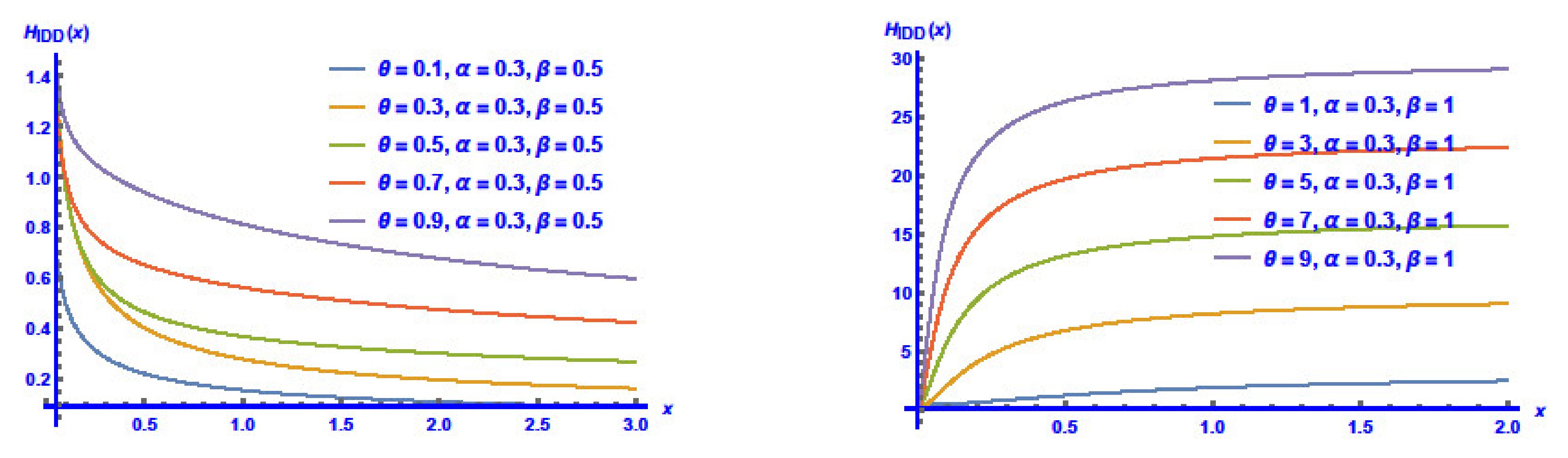
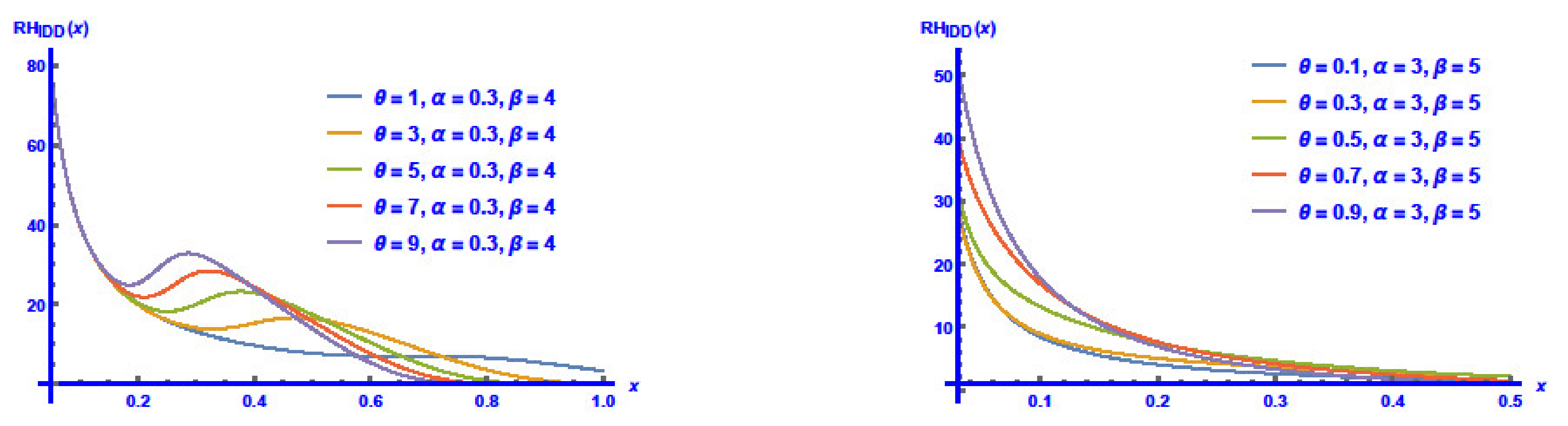
3.1. Reliability Features

The reliability functions are basic tools in analyzing the ageing and other features of any product lifetime. The survival function is the probability of an item not failing before a time x for the PDD is defined as

$$\begin{array}{ll}{S}_{PDD}(x;\alpha ,\theta ,\beta )& =1-F_{PDD}(x;\alpha ,\theta ,\beta )\\ & =1-\left(e^{\frac{\theta x^{\beta }}{\alpha }}-\frac{{\theta }^4{x}^{2\beta }+2\alpha {\theta }^3{x}^{\beta }}{2{\alpha }^2\left(2{\alpha }^2+{\theta }^2\right)}-1\right)e^{- \frac{\theta x^{\beta }}{\alpha }}\end{array}$$

(7)

The hazard function is known as the conditional probability of failure; when it has survived up to time $x\ge 0$ and for the PDD it is

$$\begin{array}{ll}{H}_{PDD}(x;\alpha ,\theta ,\beta )& =\frac{f_{PDD}(x;\alpha ,\theta ,\beta )}{1-F_{PDD}(x;\alpha ,\theta ,\beta )}\\ & =\frac{\beta \theta x^{\beta -1}\left(4{\alpha }^4+{\theta }^4{x}^{2\beta }\right)}{\alpha \left(4{\alpha }^4+2{\alpha }^2{\theta }^2+{\theta }^4{x}^{2\beta }+2\alpha {\theta }^3{x}^{\beta }\right)}.\end{array}$$

(8)

In Figure 4 and Figure 5, the plots of the survival and hazard functions are presented for some combinations of the parameters.

The reversed hazard rate function (RHF) function of the PDD is defined as

$$\begin{array}{ll}R{H}_{PDD}(x;\alpha ,\theta ,\beta )& =\frac{f_{PDD}(x;\alpha ,\theta ,\beta )}{F_{PDD}(x;\alpha ,\theta ,\beta )}\\ & =\frac{\beta \theta \left(4{\alpha }^4+{\theta }^4{x}^{2\beta }\right)}{\alpha x\left[2{\alpha }^2\left(2{\alpha }^2+{\theta }^2\right)x^{-\beta }\left(e^{\frac{\theta x^{\beta }}{\alpha }}-1\right)-2\alpha {\theta }^3-{\theta }^4{x}^{\beta }\right]}.\end{array}$$

(9)

Figure 6 shows the plots of the RHF for some PDD parameter combinations.

3.2. Moments and Related Measures

The rth moment about the origin of the PDD is defined as

$$E\left(X_{PDD}^r\right)=\frac{r {\left(\frac{\theta }{\alpha }\right)}^{-\frac{r}{\beta }}\Gamma \left(\frac{r}{\beta }\right)}{2{\beta }^3\left(2{\alpha }^2+{\theta }^2\right)}\left[4{\alpha }^2{\beta }^2+{\theta }^2(\beta +r)(2\beta +r)\right], r=1,2,3,\dots$$

(10)

For $r=1$, the mean of the PDD is

$$E(X)=\frac{\Gamma \left(\frac{1}{\beta }\right){\left(\frac{\theta }{\alpha }\right)}^{-1/\beta }}{2{\beta }^3\left(2{\alpha }^2+{\theta }^2\right)}\left[4{\alpha }^2{\beta }^2+(\beta +1)(2\beta +1){\theta }^2\right]$$

The inverse moment is defined as

$$E\left(\frac{1}{X_{PDD}^r}\right)=\frac{{\alpha }^2\Gamma \left(3-\frac{r}{\beta }\right){\left(\frac{\theta }{\alpha }\right)}^{r/\beta }\left(\frac{{\theta }^2}{{\alpha }^2}+\frac{4{\beta }^2}{2{\beta }^2+r^2-3\beta r}\right)}{2\left(2{\alpha }^2+{\theta }^2\right)},r=1,2,3,\dots$$

(11)

In

Table 1. The values of ${\mathit{\mu }}_X, {\mathit{\sigma }}_X, {\mathit{\upsilon }}_X, {\mathit{\delta }}_X,{\mathit{\kappa }}_X$ of the PDD.

$\mathit{\theta }$	${\mathit{\mu }}_{\mathit{X}}$	${\mathit{\sigma }}_{\mathit{X}}$	${\mathit{\upsilon }}_{\mathit{X}}$	${\mathit{\delta }}_{\mathit{X}}$	${\mathit{\kappa }}_{\mathit{X}}$
		$\alpha =3,\beta =3$
0.1	2.77555	1.009030	0.363542	0.169015	2.73072
0.2	2.20499	0.802234	0.363827	0.171692	2.73436
0.3	1.92918	0.702782	0.364290	0.175967	2.73998
0.4	1.75650	0.640977	0.364916	0.181573	2.74697
0.5	1.63500	0.597896	0.365686	0.188170	2.75458
0.6	1.54361	0.565844	0.366573	0.195370	2.76200
0.7	1.47185	0.540977	0.367549	0.202766	2.76842
0.8	1.41381	0.521111	0.368586	0.209956	2.77313
0.9	1.36585	0.504887	0.369651	0.216565	2.77554
1	1.32556	0.491403	0.370715	0.222266	2.77525
		$\alpha =1.5,\beta =2$
0.1	3.43900	1.799940	0.523391	0.635962	3.25885
0.2	2.44574	1.284720	0.525287	0.649080	3.29453
0.3	2.01566	1.064510	0.528119	0.666722	3.33805
0.4	1.76773	0.939490	0.531467	0.684201	3.37319
0.5	1.60568	0.858825	0.534867	0.697297	3.38757
0.6	1.49207	0.802558	0.537882	0.703147	3.37553
0.7	1.40877	0.760964	0.540162	0.700469	3.33774
0.8	1.34573	0.728658	0.541460	0.689304	3.27907
0.9	1.29682	0.702416	0.541643	0.670571	3.20624
1	1.25808	0.680214	0.540676	0.64564	3.12596

: the mean $\left({\mu }_X\right)$, coefficient of variation $\left({\upsilon }_X\right)$, standard deviation $\left({\sigma }_X\right)$, and coefficient of skewness $\left({\delta }_X\right)$ of the IDD for selected values of parameters.

Based on Table 1 it can be seen that the values of the population standard deviation and mean are decreasing as $\theta$ values are increasing. However, the ${\upsilon }_X$ and ${\kappa }_X$ values are increasing.

3.3. Quantile Function

Assume that the random variable X follows the pdf given in (6). For the PDD, the quantile function, $Q(p)$ for $0<p<1$ defined by $F\left(Q(p)\right)=p$ is the solution of the equation

$$\ln \left(\frac{{\theta }^4{\left(Q(p)\right)}^{2\beta }+2\alpha {\theta }^3{\left(Q(p)\right)}^{\beta }}{2{\alpha }^2\left(2{\alpha }^2+{\theta }^2\right)}+1\right)-\frac{\theta {\left(Q(p)\right)}^{\beta }}{\alpha }=\ln (1-p).$$

(12)

3.4. Order Statistics

Let $X_{(1)},X_{(2)},\dots ,X_{(n)}$ be the corresponding order statistics of the sample $X_1,X_2,\dots ,X_n$ selected from the CDF $F(x)$ with pdf $f(x)$. The ith order statistic, $X_{(i)}$, has the pdf given by

$$f_{(i)}(x)=\frac{n!}{(i-1)!(n-i)!}{[F(x)]}^{i-1}{[1-F(x)]}^{n-i}f(x), \mathrm{for}i=1,2,\dots ,n.$$

(13)

The pdf and cdf of the PDD is

$$f_{(i)}(x;\alpha ,\theta ,\beta )=\frac{\beta \theta m!2^{i-m-1}{x}^{\beta -1}{e}^{-\frac{\theta x^{\beta }}{\alpha }}\left(4{\alpha }^4+{\theta }^4{x}^{2\beta }\right){\left(e^{-\frac{\theta x^{\beta }}{\alpha }}\left(e^{\frac{\theta x^{\beta }}{\alpha }}-\frac{{\theta }^3{x}^{\beta }\left(2\alpha +\theta x^{\beta }\right)}{2{\alpha }^2\left(2{\alpha }^2+{\theta }^2\right)}-1\right)\right)}^{i-1}{\Psi }^{m-i}}{{\alpha }^3\left(2{\alpha }^2+{\theta }^2\right)\Gamma (i)\Gamma (1-i+m)},$$

where $\Psi =\frac{e^{-\frac{\theta x^{\beta }}{\alpha }}\left(4{\alpha }^4+2{\alpha }^2{\theta }^2+{\theta }^4{x}^{2\beta }+2\alpha {\theta }^3{x}^{\beta }\right)}{{\alpha }^2\left(2{\alpha }^2+{\theta }^2\right)}$.

The pdfs’ of lowest and largest order statistics $X_{(1)}$ and $X_{(n)}$, respectively, are

$$f_{(1)}(x;\alpha ,\theta ,\beta )=\frac{\beta \theta m{x}^{\beta -1}{e}^{-\frac{\theta x^{\beta }}{\alpha }}\left(4{\alpha }^4+{\theta }^4{x}^{2\beta }\right){\left(1-\Upsilon \right)}^{m-1}}{2{\alpha }^3\left(2{\alpha }^2+{\theta }^2\right)},$$

(14)

and

$$f_{(n)}(x;\alpha ,\theta ,\beta )=\frac{\beta \theta m{x}^{\beta -1}{e}^{-\frac{\theta x^{\beta }}{\alpha }}\left(4{\alpha }^4+{\theta }^4{x}^{2\beta }\right){\Upsilon }^{m-1}}{2{\alpha }^3\left(2{\alpha }^2+{\theta }^2\right)},$$

(15)

where $\Upsilon =e^{-\frac{\theta x^{\beta }}{\alpha }}\left(e^{\frac{\theta x^{\beta }}{\alpha }}-\frac{{\theta }^4{x}^{2\beta }+2\alpha {\theta }^3{x}^{\beta }}{2{\alpha }^2\left(2{\alpha }^2+{\theta }^2\right)}-1\right)$.

The mean and variance of $X_{(i)}$ follows the PDD are defined as

$${\mu }_{X_{(i)}}=E\left(X_{(i)}\right)={\displaystyle \underset{0}{\overset{\infty }{\int }}x f_{(i)}(x;\alpha ,\theta ,\beta )} dx \mathrm{and} {\sigma }_{X_{(i)}}^2={\displaystyle \underset{0}{\overset{\infty }{\int }}{\left(x-{\mu }_{X_{(i)}}^{}\right)}^2 f_{(i)}(x;\alpha ,\theta ,\beta ) }dx.$$

Assuming that the sample size $m=5$ and $i=1,5$,

Table 2. The ${\mathit{\mu }}_{X_{(1)}}, {\mathit{\sigma }}_{X_{(1)}}, {\mathit{\upsilon }}_{X_{(1)}}, {\mathit{\delta }}_{X_{(1)}},{\mathit{\kappa }}_{X_{(1)}}$ values of the PDD with $\alpha =3$, $\mathit{\beta }=3,$ $\mathit{i}=1$, and $m=5$.

$\mathit{\theta }$	${\mathit{\mu }}_{{\mathit{X}}_{(1)}}$	${\mathit{\sigma }}_{{\mathit{X}}_{(1)}}$	${\mathit{\upsilon }}_{{\mathit{X}}_{(1)}}$	${\mathit{\delta }}_{{\mathit{X}}_{(1)}}$	${\mathit{\kappa }}_{{\mathit{X}}_{(1)}}$
0.1	1.622990	0.589902	0.363466	0.168286	2.72972
0.2	1.288980	0.468574	0.363523	0.168835	2.73048
0.3	1.127210	0.409874	0.363619	0.169748	2.73174
0.4	1.025630	0.373076	0.363753	0.171021	2.73350
0.5	0.953892	0.347145	0.363925	0.172648	2.73575
0.6	0.899690	0.327608	0.364134	0.174622	2.73847
0.7	0.856913	0.312242	0.364380	0.176934	2.74165
0.8	0.822119	0.299796	0.364662	0.179571	2.74526
0.9	0.793190	0.289498	0.364979	0.182519	2.74928
1	0.768740	0.280844	0.365331	0.185759	2.75365

and

Table 3. The ${\mathit{\mu }}_{X_{(5)}}, {\mathit{\sigma }}_{X_{(5)}}, {\mathit{\upsilon }}_{X_{(5)}}, {\mathit{\delta }}_{X_{(5)}},{\mathit{\kappa }}_{X_{(5)}}$ values of the PDD with $\mathit{\alpha }=3$, $\mathit{\beta }=3$, $\mathit{i}=5$, and $\mathit{m}=5$.

$\mathit{\theta }$	${\mathit{\mu }}_{{\mathit{X}}_{(5)}}$	${\mathit{\sigma }}_{{\mathit{X}}_{(5)}}$	${\mathit{\upsilon }}_{{\mathit{X}}_{(5)}}$	${\mathit{\delta }}_{{\mathit{X}}_{(5)}}$	${\mathit{\kappa }}_{{\mathit{X}}_{(5)}}$
0.1	3.97393	0.694827	0.174847	0.242579	3.08906
0.2	3.15802	0.553243	0.175187	0.246439	3.09412
0.3	2.76443	0.485789	0.175729	0.252208	3.10105
0.4	2.51873	0.444399	0.176437	0.259018	3.10799
0.5	2.34650	0.415958	0.177268	0.265869	3.11300
0.6	2.21750	0.395089	0.178169	0.271784	3.11445
0.7	2.11668	0.379070	0.179087	0.275922	3.11129
0.8	2.03551	0.366333	0.179971	0.277658	3.10317
0.9	1.96872	0.355891	0.180773	0.276613	3.09036
1	1.91282	0.347083	0.181451	0.272642	3.07364

provided the values of ${\sigma }_{X_{(i)}}$, ${\mu }_{X_{(i)}}$, ${\delta }_{{\upsilon }_{X_{(i)}}}$, ${\upsilon }_{X_{(i)}}$, and ${\kappa }_{X_{(i)}}$ of the PDD for different values of parameters.

Based on Table 2 and Table 3, it is clear that the values of ${\upsilon }_{X_{(1)}}$, ${\delta }_{X_{(1)}}$, and ${\kappa }_{X_{(1)}}$ for the minimum order statistics in a sample of size 5 are increasing for increasing values of $\theta$, while the values of ${\mu }_{X_{(1)}}$ and ${\sigma }_{X_{(1)}}$ are decreasing. The same thing can be concluded to the maximum.

4. MLE with Right Censorship

Let $X={\left(X_1,X_2,\dots ,X_n\right)}^T$ be a sample that follows the PDD with the vector of parameters $\gamma ={\left(\alpha ,\theta ,\beta \right)}^T$ that can have right censored data via fixed censoring time τ. Then, each $X_i$ can be represented as $X_i=\left(x_i,{\delta }_i\right),$ with

$${\delta }_i=\left\{\begin{array}{c}0 if x_i is a censoring time \\ 1 if x_{i}is a failure time. \end{array}\right.$$

Assuming that the right censoring is not informative, the log-likelihood function can be expressed as:

$$\begin{gathered} L_n\left(\gamma \right)={{\displaystyle \sum }}_{i=1}^n{\delta }_i\mathrm{lnh}\left(x_i,\gamma \right)+{{\displaystyle \sum }}_{i=1}^{n}lnS\left(x_i,\gamma \right) \\ ={{\displaystyle \sum }}_{i=1}^n{\delta }_i\left[ln\left(\beta \theta \right)+\left(\mathsf{\beta }-1\right)ln(x_i)+\ln \left({\omega }_i\right)+\ln \left(\alpha \right)-\ln \left({\phi }_i\right)\right]+{\displaystyle \sum }_{i=1}^{n}ln\left(1-e^{-v_i}{\left(e^{v_i}-\frac{1}{2}{u}_i-1\right)}^a\right). \end{gathered}$$

(16)

We pose, ${\phi }_i=4{\alpha }^4+2{\alpha }^2{\theta }^2+{\theta }^4{x}_i^{2\beta }+2\alpha {\theta }^3{x}_i^{\beta }, u_i=\frac{{\theta }^4{x}_i^{2\beta }+2\alpha {\theta }^3{x}_i^{\beta }}{{\alpha }^2\left(2{\alpha }^2+{\theta }^2\right)}, v_i=\frac{\theta x_i^{\beta }}{\alpha }, {\omega }_i=4{\alpha }^4+{\theta }^4{x}_i^{2\beta }.$ The nonlinear following score equations are used to obtain the maximum likelihood estimators (MLE) $\widehat{\alpha }, \widehat{\beta }$, and $\widehat{\theta }$ of the unknown parameters $\alpha$, $\beta$, and $\theta ,$ as

$$\frac{\partial L}{\partial \alpha }={{\displaystyle \sum }}_{i=1}^n{\delta }_i\left[\frac{16{\alpha }^3}{{\omega }_i}-\frac{1}{\alpha }-\frac{1}{{\phi }_i}\left(16{\alpha }^3+4\alpha {\theta }^2+2{\theta }^3{x}_i^{\beta }\right)\right]-{{\displaystyle \sum }}_{i=1}^n\frac{1}{S\left(x_i,\gamma \right)}\left(\frac{v_i}{\alpha }\left(1-\frac{1}{2}{u}_i{e}^{-v_i}\right)-e^{-v_i}\left(\frac{v_i{e}^{v_i}}{\alpha }-\frac{{\theta }^3{x}_i^{\beta }}{{\alpha }^2\left(2{\alpha }^2+{\theta }^2\right)}+\frac{u_i}{\alpha }+2\alpha u_i\right)\right),$$

$$\frac{\partial L}{\partial \theta }={{\displaystyle \sum }}_{i=1}^n{\delta }_i\left[\frac{1}{\theta }+\frac{4{\theta }^3{x}_i^{2\beta }}{{\omega }_i}-\frac{1}{{\phi }_i}\left(4{\alpha }^2\theta +4{\theta }^3{x}_i^{2\beta }+6\alpha {\theta }^2{x}_i^{\beta }\right)\right]+{{\displaystyle \sum }}_{i=1}^n\frac{1}{S\left(x_i,\gamma \right)}\left(\frac{x_i^{\beta }}{\alpha }\left(1-\frac{1}{2}{u}_i{e}^{-v_i}\right)-e^{-v_i}\left(\frac{x_i^{\beta }{e}^{v_i}}{\alpha }-\frac{2{\theta }^3{x}_i^{2\beta }+3\alpha {\theta }^2{x}_i^{\beta }}{{\alpha }^2\left(2{\alpha }^2+{\theta }^2\right)}+\theta u_i\right)\right),$$

$$\begin{array}{c}\frac{\partial L}{\partial \beta }={\sum }_{i=1}^n{\delta }_i\left[\frac{1}{\beta }+ln\left(x_i\right)+\frac{2{\theta }^4{x}_i^{2\beta }ln\left(x_i\right)}{{\omega }_i}-\frac{1}{{\phi }_i}\left(2{\theta }^4{x}_i^{2\beta }ln\left(x_i\right)+2\alpha {\theta }^3{x}_i^{\beta }ln\left(x_i\right)\right)\right]-\\ {\sum }_{i=1}^n\frac{1}{S\left(x_i,\gamma \right)}\left(v_{i}ln\left(x_i\right)\left(1-\frac{1}{2}{u}_i{e}^{-v_i}\right)-e^{-v_i}\left(v_{i}ln\left(x_i\right)e^{v_i}-\frac{{\theta }^4{x}_i^{2\beta }ln\left(x_i\right)+\alpha {\theta }^3{x}_i^{\beta }ln\left(x_i\right)}{{\alpha }^2\left(2{\alpha }^2+{\theta }^2\right)}\right)\right)\end{array}$$

The explicit forms of $\widehat{\alpha }, \widehat{\beta }$, and $\widehat{\theta }$ cannot be gained, so we may use some numerical methods to obtain them.

5. Right Censored Data Test Statistic

Let $X₁,X_2,\dots ,X_n$ be n i.i.d. random variables assembled into $r$ classes $I_i$. To determine whether a parametric model F₀ is adequate, let

$$H_0: P\left(X_i\le x{H}_0\right)=F_0\left(x;\gamma \right),x\ge 0, \gamma ={\left({\gamma }_1,{\gamma }_{2,}\dots ,{\gamma }_s\right)}^T\in \Theta \subset R^s,$$

provided that the data are right censored with unknown vector $\gamma$ [17] recommended a statistic test Y² based on

$$Z_j=\frac{1}{\sqrt{n}}\left(U_j-e_j\right), j=1,2,\dots ,r, with r>s.$$

This shows the dissimilarities between observed and expected numbers of failures ($U_j$ and $e_j$) to be in these grouped intervals $I_j=\left(p_{j-1},p_j\right]$, where $p_0=0, p_r=\tau$, and τ is a finite time. The researchers utilized $p_j$ as functions random data, such as the r intervals selected, which have the same expected numbers of failures $e_j$. The statistic Y² is defined by

$$Y^2=Z^T\widehat{\Sigma }{}^{-}Z={{\displaystyle \sum }}_{i=1}^r\frac{{\left(U_j-e_j\right)}^2}{U_j}+Q,$$

where $\widehat{\Sigma } is a$ covariance matrix with generalized inverse ${\widehat{\Sigma }}^{-} Z={\left(Z_1,Z_2,\dots ,Z_k\right)}^T$,$Q=W^T{\widehat{G}}^{-}W,$ $\widehat{A_j}=\frac{U_j}{n},$ $U_j={\displaystyle \sum }_{i:X_i\in I_j}{\delta }_i$, $W={\left(W_1,W_2,\dots ,W_s\right)}^T,$ $\widehat{G}={\left[{\widehat{g}}_{l{l}^{\prime }}\right]}_{s\times s},$ ${\widehat{g}}_{l{l}^{\prime }}={\widehat{i}}_{l{l}^{\prime }}-{\displaystyle \sum }_{j=1}^r{\widehat{C}}_{lJ}{\widehat{G}}_{l^{\prime }J}{\widehat{A}}_J^{-1}$, ${\widehat{C}}_{lj}=\frac{1}{n}{\displaystyle \sum }_{i:X_i\in I_j}{\delta }_i\frac{\partial lnh\left(x_i,\widehat{\gamma }\right)}{\partial \gamma },$ ${\widehat{i}}_{l{l}^{\prime }}=\frac{1}{n}{\displaystyle \sum }_{i=1}^n{\delta }_i\frac{\partial lnh\left(x_i,\widehat{\gamma }\right)}{\partial {\gamma }_l}\frac{\partial lnh\left(x_i,\widehat{\gamma }\right)}{\partial {\gamma }_{l^{\prime }}}$, ${\widehat{W}}_l={\displaystyle \sum }_{j=1}^r{\widehat{C}}_{lJ}{\widehat{A}}_J^{-1}{Z}_j$, $l,l^{\prime }=12,\dots ,s$, $and \widehat{\gamma }$ is the MLE of $\gamma$ for primary non-grouped data.

The statistic Y² under the null hypothesis H₀ has a chi-square limiting distribution with $r=rank\left(\Sigma \right)$ degrees of freedom. In [18], the explanation and usages of improved chi-square tests are covered. Now, $I_j$ are considered as data functions for grouped data into j classes with $p_{j }$ interval limits, and it is defined by

$${\widehat{p}}_j=H^{-1}\left(\frac{E_j-{{\displaystyle \sum }}_{l=1}^{i-1}H\left(x_l,\widehat{\gamma }\right)}{n-i+1},\widehat{\gamma }\right), {\widehat{p}}_j=\max \left(X_{\left(n\right)},\tau \right),$$

such as $e_j=\frac{E_r}{r}$ to fall into these intervals for any j, with $E_r={\displaystyle \sum }_{i=1}^{n}H\left(x_i,\gamma \right)$. The statistic test $Y_n^2$ has a chi-square distribution (see [18]).

5.1. Criteria Test for PDD

On the basis of the statistic Y², we create an adapted chi-squared-type GOF test to test the null hypothesis H₀ that the data follow the PDD model. Assume that τ is a finite period of time and that the observed data are divided into $r>s$ subintervals $I_j=\left(p_{j-1},p_j\right]$ of $\left[0,\tau \right]$. Then, $e_j$ are calculated as the limit intervals $p_j$ are treated as random variables, such that the $e_j$ in each interval $I_j$ are equal. Hence, the expected numbers of failures are

$$E_j=-\frac{j}{r-1}{\displaystyle \sum }_{i=1}^n\ln \left\{1-e^{-v_i}{\left(e^{v_i}-\frac{1}{2}{u}_i-1\right)}^a\right\}, j=1,2,\dots ,r-1.$$

5.2. Estimated Matrix $\widehat{W}$ et $\widehat{C}$

The elements of the estimated matrix $\widehat{W}$ are obtained from the estimated matrix $\widehat{C}$, where:

$${\widehat{C}}_{1j}=\frac{1}{n}{\displaystyle \sum }_{i:x_i\in I_j}^n{\delta }_i\left[\frac{16{\alpha }^3}{{\omega }_i}-\frac{1}{\alpha }-\frac{1}{{\phi }_i}\left(16{\alpha }^3+4\alpha {\theta }^2+2{\theta }^3{x}_i^{\beta }\right)\right],$$

$${\widehat{C}}_{2j}=\frac{1}{n}{\displaystyle \sum }_{i:x_i\in I_j}^n{\delta }_i\left[\frac{1}{\theta }+\frac{4{\theta }^3{x}_i^{2\beta }}{{\omega }_i}-\frac{1}{{\phi }_i}\left(4{\alpha }^2\theta +4{\theta }^3{x}_i^{2\beta }+6\alpha {\theta }^2{x}_i^{\beta }\right)\right],$$

$${\widehat{C}}_{3j}=\frac{1}{n}{\displaystyle \sum }_{i:x_i\in I_j}^n{\delta }_i\left[\frac{1}{\beta }+\ln \left(x_i\right)+\frac{2{\theta }^4{x}_i^{2\beta }\ln \left(x_i\right)}{{\omega }_i}-\frac{1}{{\phi }_i}\left(2{\theta }^4{x}_i^{2\beta }\ln \left(x_i\right)+2\alpha {\theta }^3{x}_i^{\beta }\ln \left(x_i\right)\right)\right],$$

$${\widehat{W}}_l={\displaystyle \sum }_{j=1}^r{\widehat{C}}_{lJ}{\widehat{A}}_J^{-1}{Z}_j, l,l^{\prime }=1,2,3, \mathrm{and} j=1,2,\dots ,r.$$

5.3. Estimated Matrix $\widehat{G}$

The estimated matrix $\widehat{G}={\left[{\widehat{g}}_{l{l}^{\prime }}\right]}_{3\times 3}$ is defined by

$${\widehat{g}}_{l{l}^{\prime }}={\widehat{i}}_{l{l}^{\prime }}-{\displaystyle \sum }_{j=1}^r{\widehat{C}}_{lJ}{\widehat{G}}_{l^{\prime }J}{\widehat{A}}_J^{-1},$$

where

$${\widehat{i}}_{l{l}^{\prime }}=\frac{1}{n}{\displaystyle \sum }_{i=1}^n{\delta }_i\frac{\partial lnh\left(x_i,\widehat{\gamma }\right)}{\partial {\gamma }_l}\frac{\partial lnh\left(x_i,\widehat{\gamma }\right)}{\partial {\gamma }_{l^{\prime }}}, l,l^{\prime }=1,2,3.$$

Therefore, the quadratic form of $Y_n^{}\left(\widehat{\gamma }\right)$ can be gained as:

$$Y_n^2\left(\widehat{\gamma }\right)={\displaystyle \sum }_{j=1}^r\frac{{\left(U_j-e_j\right)}^2}{U_j}+{\widehat{W}}^T{\left[{\widehat{i}}_{l{l}^{\prime }}-{\displaystyle \sum }_{j=1}^r{\widehat{C}}_{lJ}{\widehat{G}}_{l^{\prime }J}{\widehat{A}}_J^{-1}\right]}^{-1}\widehat{W}.$$

(17)

6. Estimations Are Applications

Here, the MLE scheme is considered to estimate the distribution parameters and an example of a real data set is carried out for explanation of the applicability of the distribution.

6.1. Maximum Likelihood Estimation

In this part, $N=10,000$ right censored samples for parameters $\alpha =3$, $\beta =4, \mathrm{and} \theta =0.1, \mathrm{and}$ different sizes ($n=25, 50, 130, 350, 500$) are generated from the PDD model. We compute the MLE’s of the unknown parameters and their mean squared errors (MSE) using the R statistical package and the Barzilai–Borwein (BB) algorithm [19].

Table 4. Mean simulated values of the MLEs of $\widehat{\gamma }$ with corresponding MSE.

N	n = 25	n = 50	n = 130	n = 350	n = 500
$\widehat{\alpha }$	2.9602	2.9677	2.9707	2.9813	2.9983
MSE	0.0062	0.0049	0.0035	0.0021	0.0012
$\widehat{ \beta }$	4.0422	4.0314	4.0250	4.0183	4.0034
MSE	0.0083	0.0062	0.0055	0.0039	0.0025
$\widehat{\theta }$	0.9753	0.9789	0.9802	0.9898	0.9933
MSE	0.0072	0.0057	0.0038	0.0028	0.0017

presents the outcomes.

The MLE of the estimated parameter values, presented in Table 4, agree closely with the true parameter values.

6.2. Application to Survival Data

Reference [20] gave data from a laboratory analysis in which the vaginas of rats are painted with the carcinogenic DMBA, and the number of T days until onset of carcinoma are recorded. The data concern a group of 19 rats (Group 1 in Pike’s article). The two observations with asterisks are censorship times. The data set is: 164, 143, 188, 190, 188, 192, 209, 206, 213, 216, 216 *, 220, 227, 234, 230, 244 *, 246, 265, and 304. (* indicates the censorship).

We use the statistic test given above to examine if these data are modeled by PDD, and at that end, we first calculate the MLE of the unknown parameters

$$\gamma ={\left(\alpha ,\beta ,\theta \right)}^T={\left(3.5677;5.3696; 0.0973\right)}^T.$$

(18)

The data are grouped into $r=4$ intervals $I_j$, and the essential calculus is in the following

Table 5. Values of $p_j,e_j,U_j,{\widehat{C}}_{1j},{\widehat{C}}_{2j},{\widehat{C}}_{3j}$.

$p_j$	189	218	245	304
$U_j$	4	7	5	3
$e_j$	0.5012	0.5012	0.5012	0.5012
${\widehat{C}}_{1j}$	1.2262	2.6789	1.9501	2.1657
${\widehat{C}}_{2j}$	0.9346	1.9832	2.4702	4.1017
${\widehat{C}}_{3j}$	−3.4764	−2.6677	−1.4667	−2.3824

.

Then, we obtain the value of the statistic test $Y_n^2 as$:

$$Y_n^2=X^2+Q=4.8532+2.6134=7.4666$$

(19)

For a significance level of ε = 0.05, the critical value ${\chi }_4^2=9.4877$ is superior to the value of $Y_n^2$=$7.4666$, so we can say that the recommended model PDD fits these data.

7. Conclusions

The power Darna distribution is presented in this paper. The PDD distribution has some interesting statistical features. The B-N goodness-of-fit test under the right-censored situation is examined and implemented for the distributional validation of a modified kind of statistic. Based on the B-N chi-square GOF test, a revised, modified GOF test is presented. The censored Barzilai–Borwein algorithm is used in a thorough simulation exercise to evaluate the new test. Actual and right-censored sets of data are tested using a modified B-N test. An application to carcinogenic DMBA in the vaginas of rats is considered for illustration. Future research could investigate the PDD in different situations and estimate its parameters using techniques such as ranked set sampling [21,22].

References

1. Mudholkar, G.S.; Srivastava, D.K. Exponentiated Weibull family for analyzing bathtub failure-rate data. IEEE Trans. Reliab. 1993, 42, 299–302. [Google Scholar] [CrossRef]
2. Marshall, A.W.; Olkin, I. A new method for adding a parameter to a family of distributions with application to the exponential and Weibull families. Biometrika 1997, 84, 641–652. [Google Scholar] [CrossRef]
3. Mahdavi, A.; Kundu, D. A new method for generating distributions with an application to exponential distribution. Commun. Stat. Theory Methods 2017, 46, 6543–6557. [Google Scholar] [CrossRef]
4. Granzotto, D.; Louzada, F.; Balakrishnan, N. Cubic rank trans- muted distributions: Inferential issues and applications. J. Stat. Comput. Simul. 2017, 87, 2760–2778. [Google Scholar] [CrossRef]
5. Abd EL-Kade, R.; AL-Dayian, G.; AL-Gendy, S. Inverted Pareto type I distribution: Properties and estimation. J. Fac. Commer. AL Azhar Univ. Girls Branch 2003, 21, 19–40. [Google Scholar]
6. Al-Dayian, G. Inverted pareto type ii distribution: Properties and estimation. J. Fac. Commer. AL Azhar Univ. Girls Branch 2004, 22, 1–18. [Google Scholar]
7. Sharma, V.K.; Singh, S.K.; Singh, U.; Agiwal, V. The inverse Lindley distribution: A stress-strength reliability model with application to head and neck cancer data. J. Ind. Prod. Eng. 2015, 32, 162–173. [Google Scholar] [CrossRef]
8. Abd AL-Fattah, A.; El-Helbawy, A.; Al-Dayian, G. Inverted Kumaraswamy distribution: Properties and estimation. Pak. J. Stat. 2017, 33, 37–61. [Google Scholar]
9. Ghitany, M.; Al-Mutairi, D.K.; Balakrishnan, N.; Al-Enezi, L. Power Lindley distribution and associated inference. Comput. Stat. Data Anal. 2013, 64, 20–33. [Google Scholar] [CrossRef]
10. Rady, E.-H.A.; Hassanein, W.; Elhaddad, T. The power Lomax distribution with an application to bladder cancer data. SpringerPlus 2016, 5, 1838. [Google Scholar] [CrossRef]
11. Hassan, A.S.; Assar, S.M.; Abdelghaffar, A.M. Statistical properties and estimation of power-transmuted inverse Rayleigh distribution. Stat. Transit. New Ser. 2020, 21, 93–107. [Google Scholar] [CrossRef]
12. Shraa, D.H.; Al-Omari, A.I. Darna distribution: Properties and application. Electron. J. Appl. Stat. Anal. 2019, 12, 520–541. [Google Scholar]
13. Habib, M.; Thomas, D. Chi-square goodness-if-fit tests for randomly censored data. Ann. Stat. 1986, 14, 759–765. [Google Scholar] [CrossRef]
14. Hollander, M.; Pena, E.A. A chi-squared goodness-of-fit test for randomly censored data. J. Am. Stat. Assoc. 1992, 87, 458–463. [Google Scholar] [CrossRef]
15. Galanova, N.; Lemeshko, B.Y.; Chimitova, E. Using nonparametric goodness-of-fit tests to validate accelerated failure time models. Optoelectron. Instrum. Data Processing 2012, 48, 580–592. [Google Scholar] [CrossRef]
16. Bagdonavičius, V.; Nikulin, M. Chi-squared tests for general composite hypotheses from censored samples. Comptes Rendus Math. 2011, 349, 219–223. [Google Scholar] [CrossRef]
17. Bagdonavicius, V.; Nikulin, M. Chi-squared goodness-of-fit test for right censored data. Int. J. Appl. Math. Stat. 2011, 24, 1–11. [Google Scholar]
18. Voinov, V.; Nikulin, M.; Balakrishnan, N. Chi-Squared Goodness of Fit Tests with Applications; Academic Press: Cambridge, MA, USA; Elsevier: Amsterdam, The Netherlands, 2013. [Google Scholar]
19. Ravi, V.; Gilbert, P.D. BB: An R package for solving a large system of nonlinear equations and for optimizing a high-dimensional nonlinear objective function. J. Statist. Softw. 2009, 32, 1–26. [Google Scholar]
20. Pike, M. A method of analysis of a certain class of experiments in carcinogenesis. Biometrics 1966, 22, 142–161. [Google Scholar] [CrossRef] [PubMed]
21. Al-Omari, A.I. Maximum likelihood estimation in location-scale families using varied L ranked set sampling. RAIRO-Oper. Res. 2021, 55, S2759–S2771. [Google Scholar] [CrossRef]
22. Haq, A.; Brown, J.; Moltchanova, E.; Al-Omari, A.I. Paired double ranked set sampling. Commun. Stat. Theory Methods 2016, 45, 2873–2889. [Google Scholar] [CrossRef]
Figure 1. Plots of the CDF of PDD for varying the value of α ,   β ,   θ .
Applsci 12 08272 g001
Figure 2. Pdf plots of the PDD with various values of parameters.
Applsci 12 08272 g002
Figure 3. Plots of the PDD and DD with various values of parameters.
Applsci 12 08272 g003
Figure 4. The survival function plots of the PDD for some values of parameters.
Applsci 12 08272 g004
Figure 5. The hazard function plots of the PDD for some values of parameters.
Applsci 12 08272 g005
Figure 6. The RHF plots of PDD for different values of parameters.
Applsci 12 08272 g006