1. Introduction
In the positioning requirements of unmanned driving, the global positioning system based on GPS and differential GPS has the characteristics of high efficiency and accuracy. However, in tunnels, heavily blocked roads, urban canyons and other roads, GPS signals are severely affected and cannot complete the positioning work. At this time, SLAM technology has important application value [
1,
2]. Compared with other sensors, vision technology can better combine perceptual information and play a major role in unmanned vehicle applications. Vision sensors can detect lane lines [
3,
4], road signs [
5,
6] and other information required for vehicle driving through deep learning and other technologies. Under structured roads, good detection results can be achieved for unmanned driving needs, through accurate local positioning methods, such as lane keeping [
7,
8], navigable area navigation [
9], etc. However, this local navigation method still needs SLAM and other methods to supplement and judge the positioning results due to the instability of detection. The visual SLAM system mainly includes two forms: monocular [
10,
11,
12,
13] and multi-eye [
14]. Multi-eye vision requires complex calculations and a large amount of matching point information. Monocular vision is simple and stable, but it lacks the true scale. The SLAM system [
15,
16] combined with a monocular camera and IMU has better adaptability, and it can provide short-term stable positioning results in scenarios where GPS is missing. However, in the application of unmanned vehicles, the positioning result error will continue to increase due to accumulated errors and IMU divergence, and the trajectory of unmanned vehicles can rarely be corrected by loopback [
17].
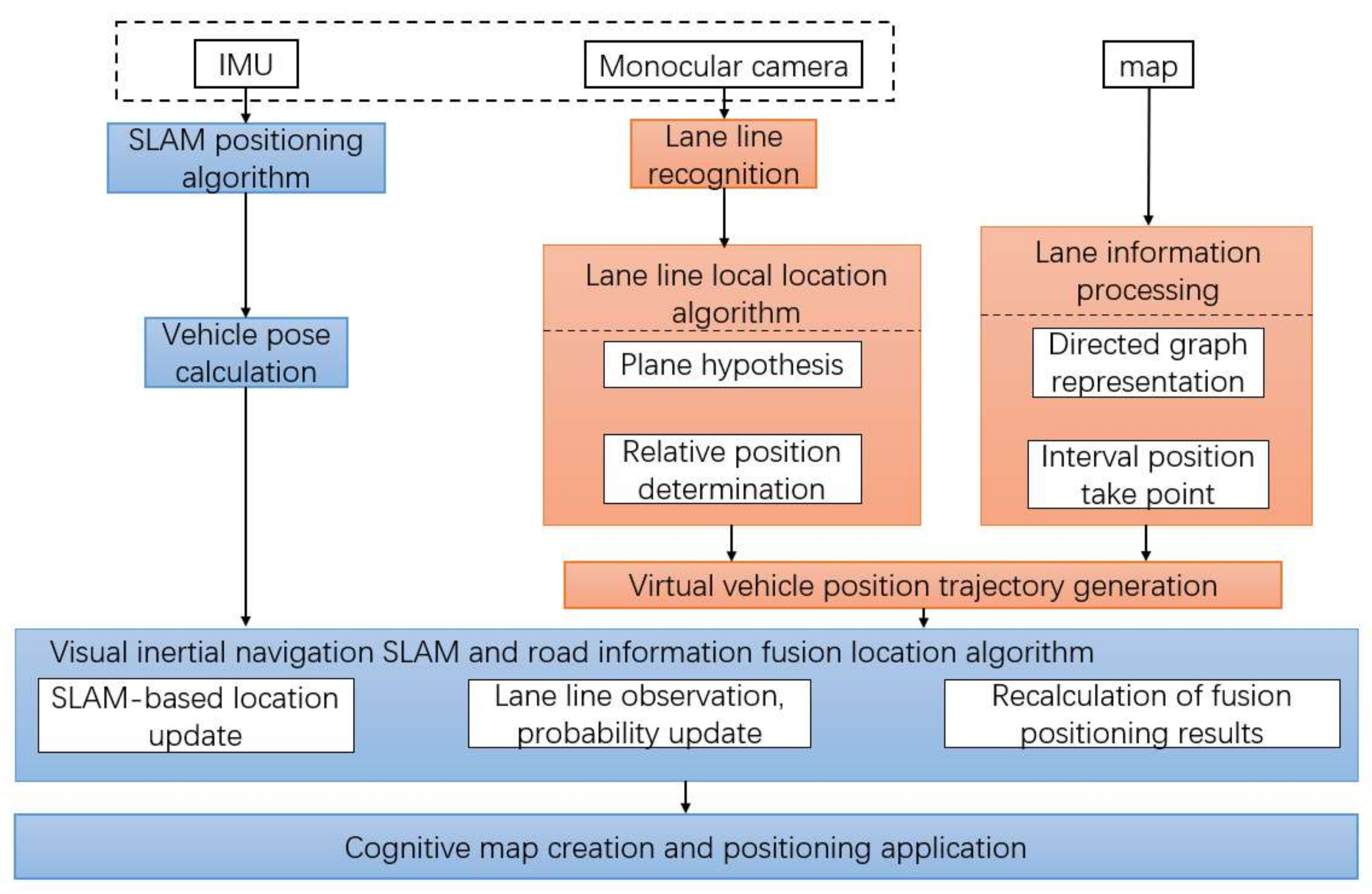
To address the problem of accumulating errors in SLAM for unmanned vehicles, we introduce map-prior information for SLAM repositioning. The accumulated visual errors and IMU integration lead to increasing SLAM localization errors, while the single movement of an unmanned vehicle rarely passes through repeated positions and cannot be corrected by traditional loopback. We adopt a maximum a posteriori probability approach to represent its own position through a probability distribution; use the localization result output of SLAM as the position update incentive; use the map midway width, lane angle and road position information as a priori; and adopt a prediction-update model to calculate the probability distribution of vehicle position through the recognized lane line perception information. It is worth noting that, different from the general map trajectory mapping [
18] which compares a certain segment of motion results with map information, the semantic SLAM [
19,
20] method increases the positioning accuracy by adding the inter-frame connection of semantic information. The algorithm flow is shown in
Figure 1.
3. Fusion of Lane Location Information and SLAM Positioning Algorithm
The above-mentioned lane line detection and representation are sufficient to enable unmanned vehicles to complete lane keeping and steering functions, but it is still impossible to determine the specific global position of the lane where the unmanned vehicle is located. Therefore, the global consistent positioning method of SLAM needs to be considered. This paper uses a SLAM system that combines vision and inertial navigation. Based on the algorithm [
15], IMU and monocular camera are used to complete the front-end output process of SLAM. Different from the indoor SLAM algorithm, it is difficult to have enough loop information during the driving process of the unmanned vehicle. Therefore, combining the timely position information which is provided by the SLAM and the map information is an important way to create an artificial loop. In this paper, by correlating the detected lane and position information, a prediction-update model is used to realize the fusion of SLAM positioning information and vehicle map lane position.
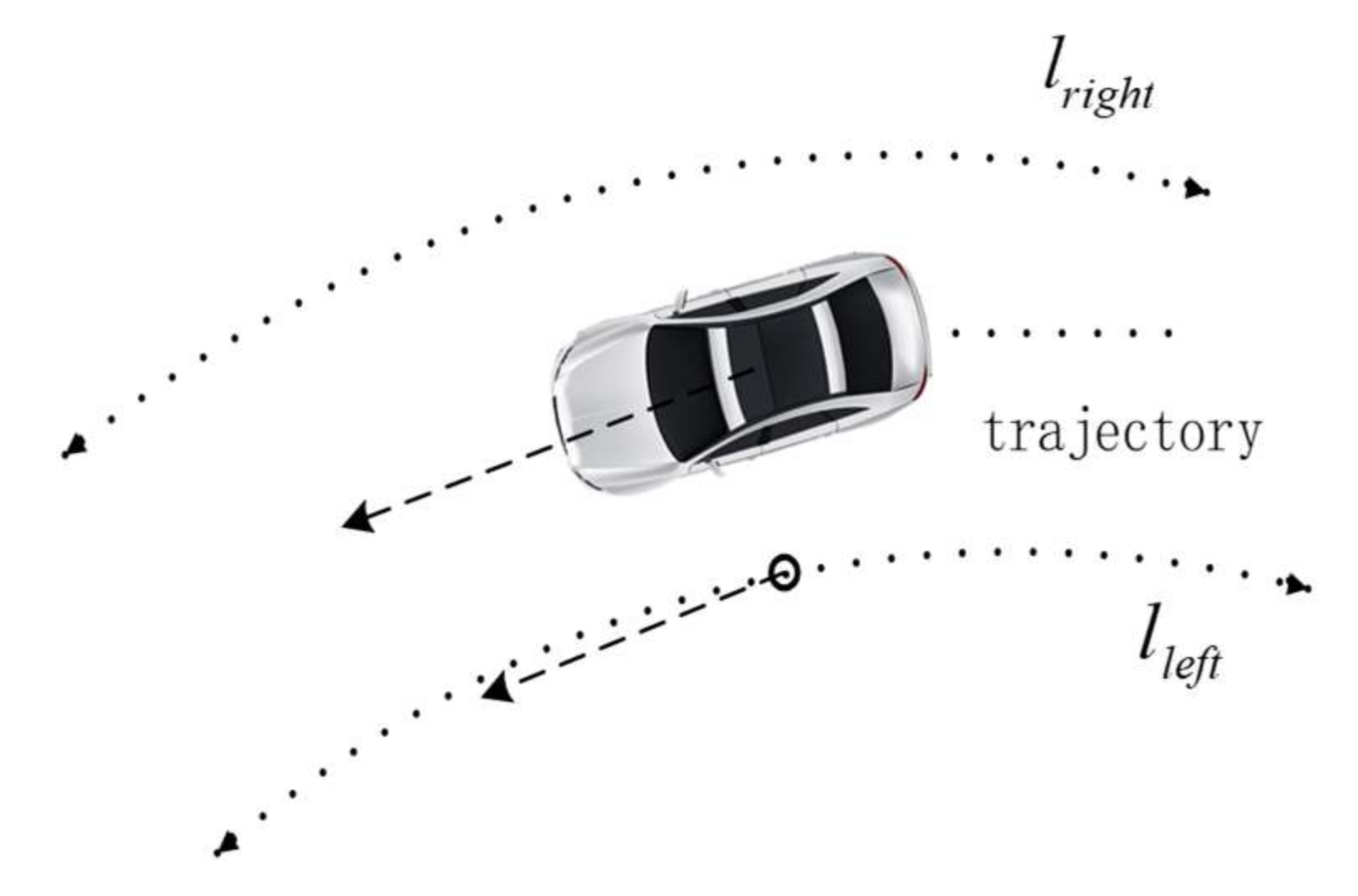
At each moment of fusion positioning, the result of the above local positioning is used to obtain the virtual trajectory of the vehicle parallel to the lanes of the map. Each point stored in the directed graph of the map is translated to this virtual trajectory in the same way. After the line localization result is updated, this operation performs the same processing on the virtual trajectory and the map point.
In the rest of this section, the map point mentioned refers to the point information stored in the directed graph on the map, and the candidate point refers to the map point where the vehicle has a greater probability of being at this position. The candidate points are on the virtual track obtained after each update of the distance from the lane line. The core of this method lies in the update of candidate points. Probability is used to update the candidate points and realize the positioning function.
3.1. Initialization of Starting Point Position
The result of SLAM output is the position in the body coordinate system, and the road information stored on the map is the global latitude and longitude. Therefore, first obtain the latitude and longitude coordinates and heading angle at the moment through manual positioning and location recognition at the starting point. The SLAM output is converted to latitude and longitude coordinates.
First, take the current position as the center point, and take the nearest K points in the map stored in the directed graph along the current yaw angle a candidate points for the vehicle’s possible poses. Each time a new candidate point is obtained, the probability of the vehicle at K candidate points on the map will be calculated, and the candidate point with the highest probability will be output as the vehicle position. At the initial moment, it is assumed that the probability of the vehicle at each candidate point of the map obeys the Gaussian distribution and satisfies the following formula.
represents the probability that the vehicle position is at the current candidate point , represents the covariance matrix, which is set to the identity matrix at the initial moment; and is the state variable at this time. At the initial moment, it only contains the position in the world coordinate system; is the map position obtained by initial positioning, that is, the center point of the Gaussian distribution; and the dimension of is 2. At the same time, in order to avoid the influence of extreme conditions, after each probability calculation is completed, the probability of K points is normalized.
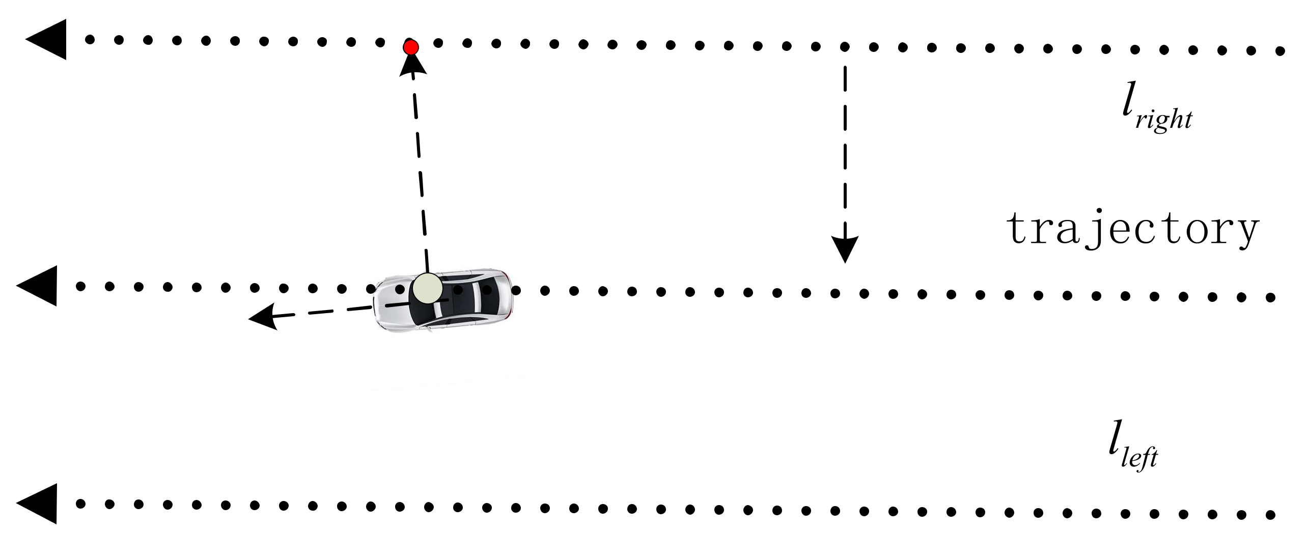
3.2. Location Prediction Based on SLAM Information
As shown in
Figure 4. Firstly,
is still obtained through the local positioning method of the lane line. The map candidate points are translated to the current vehicle position to generate a virtual trajectory, and a batch of new map candidate points are obtained. Taking the motion information from SLAM as the predicted excitation
,
is the representation of the SLAM position change in the world coordinate system. After obtaining the changes combined with the SLAM positioning information, the position is updated on the basis of the K map candidate point positions obtained after the last calculation. For each candidate point, with the updated position
as the center, select
K points according to the nearest neighbor principle, and calculate the probability of the updated position of the vehicle at each candidate point.
represents the probability that the vehicle is at position at time k + 1. For each candidate point at time k, K new candidate points are obtained and normalized. Through the prediction of K candidate points, probability updates can be generated, and new candidate points can be obtained. Through K calculations, the probability of the vehicle at each new candidate point is accumulated and normalized. Each candidate point has direction and position information in the representation of the directed graph, and can be established by constraining by the position of the lane line, the angle between the observed lane projection, the vehicle coordinate system and the map point contact, and update the probability of these results as observations.
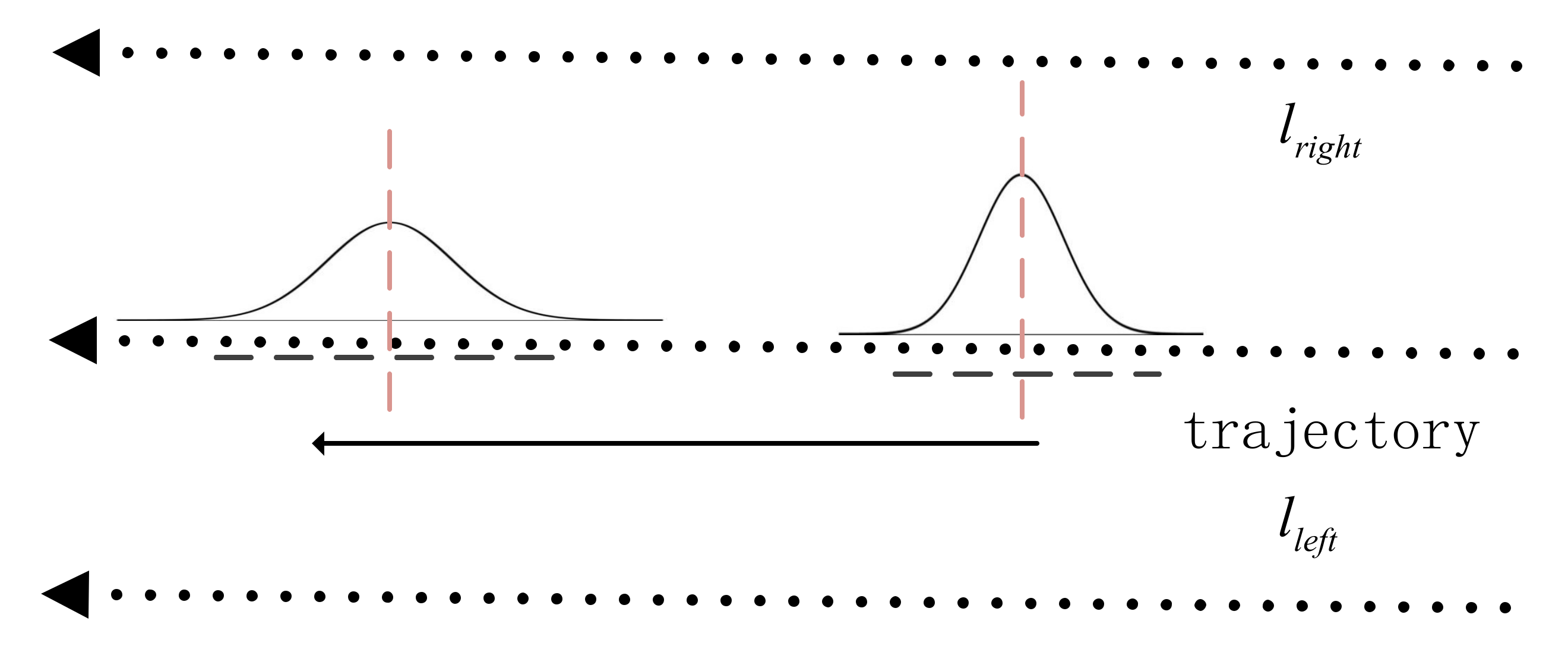
3.3. Location Probability Update Based on Lane Line Observation
As shown in
Figure 5. This link needs to select the
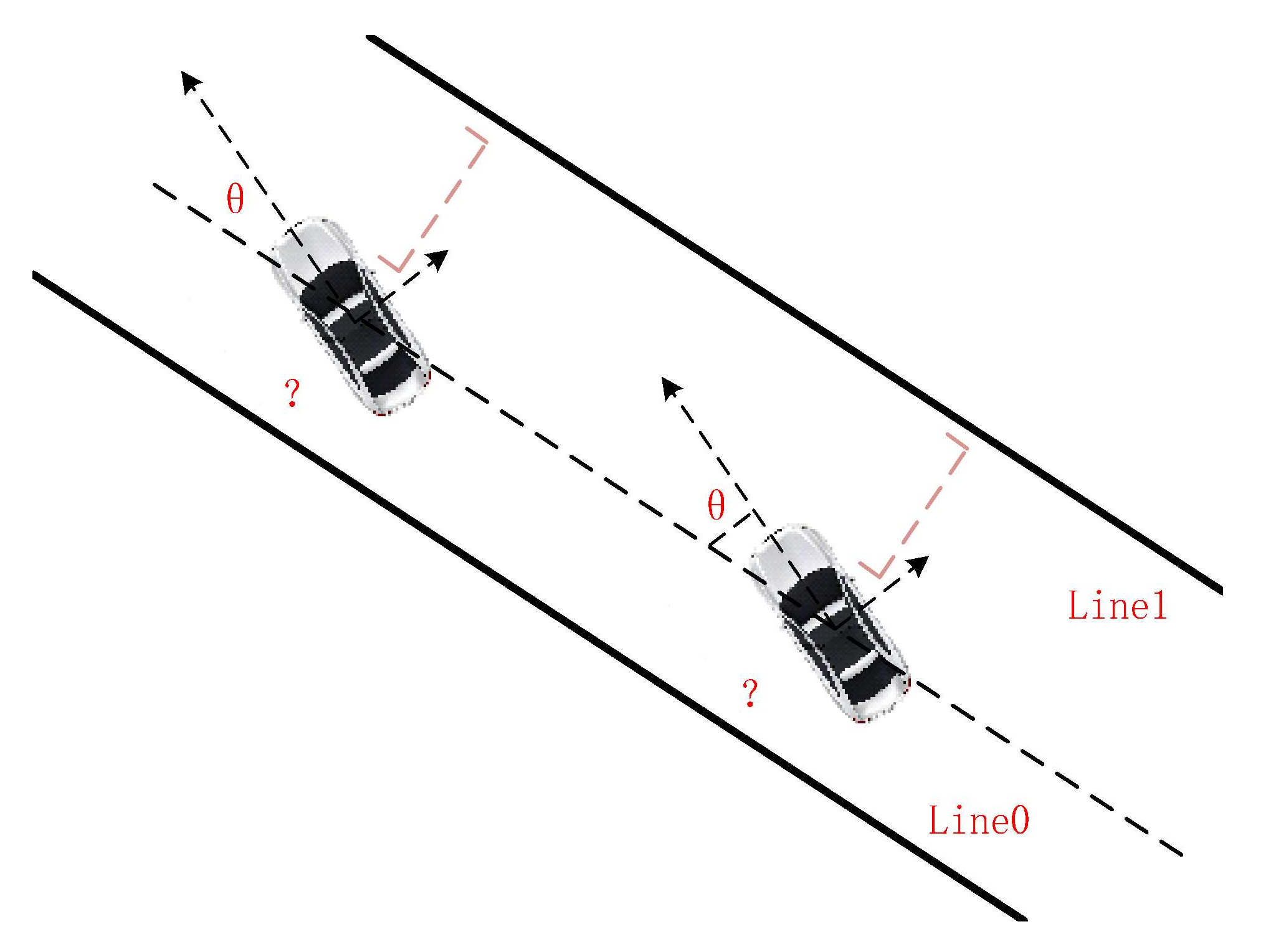
K points with the highest probability among the predicted candidate points. Since the lane of the map has been discretized by these points, first find the only corresponding lane line point
in the tangent direction of the vehicle attitude. This point is in the lane line stored in the original directed graph, representing the projection of the vehicle’s position on the lane line map point at this time. Observation is carried out at each candidate point, and the observed value is the distance
, the angle of the lane line
and the position of the vehicle body, which is obtained by the local positioning method of the lane line.
The points in the map save the position information (x, y) and tangential angle information of each point, which can be combined with and angle . According to the current position of the vehicle, the distance to the map point in the direction of the tangential lane line can be obtained , represents the currently calculated map candidate point. represents the angle between the vehicle and the lane line. Set the current yaw angle of the vehicle as that which is output by the SLAM system and converted into world coordinates in the initialization process. At this time, the calculated lane angle is . It is worth noting that the lane line detection section above has fitted the lane line to the lane line closest to the current vehicle, so the probability of the vehicle at the current candidate point can be described by the probabilistic equation of the above parameters.
represents the probability of the latest position candidate point obtained by the vehicle after the above prediction, which is a correct update of
. The observations
used to describe the vehicle at this candidate point include the latitude and longitude position
, the map distance point from the vehicle to the lane line, and the current. The error of the local positioning result
, as well as the error of the angle
stored by the candidate point and the current observation angle, are a total of four-dimensional variables. The matrix
represents the covariance matrix. This paper assumes that each variable is distributed independently.
is a diagonal matrix with a dimension of 4 × 4, and the four diagonal corners
are, respectively, from the upper left to the lower right corner.
is the position variance,
is the angle variance with In radians and
represents the error of the current local positioning. Due to abnormal conditions such as detection failure, a robust kernel function
is added to prevent the unstable influence caused by the wrong local positioning, and it is eliminated when the error is too large. Finally, all the candidate point probabilities are updated.
In this paper, only one lane line is used as the observation. In the experiment, the accuracy improvement produced by the use of multiple lane lines is very small, and at the same time, it generates a lot of problems, so that the data association difficult to determine. Therefore, the above operation only performs the observation update of one lane line. This paper takes the nearest left end lane line as an example. After the probability update is obtained, the K points with the highest probability are selected from the predicted candidate points as the current new candidate points and normalized.
3.4. Result Processing and Output
After each observation update, the value with the highest probability
is output as the current vehicle position relocation result. At the same time, according to the position and direction angle of , calculate the position of the current point and the original lane line point in the map, so as to obtain the updated local positioning result . Take the latest result obtained as the latest value and repeat the above steps to update the position.
The above results probabilistically process the position of the vehicle on the map. However, there are still some special problems that cause the system to fail to run, or make the convergence speed too slow:
a. There are not enough candidate points, or the probability value of the candidate points is too small.
When the system moves in a straight line for a long time, because the accumulated error is already large, the selected points are often limited to a certain range, resulting in the inability to update the position. The solution is that when the probability of a candidate point is too small, delete this point and let expand the value of the covariance matrix to facilitate the selection of more points next time.
b. Lack of significant optimal points.
If there is no significant optimal point , the probability difference of each candidate point is small at this time, and it is easy to fall into the local optimal value and cannot move forward. In places with obvious detours (intersections exceeding 90 degrees), the change of angle information is too obvious. Two candidate points with very different positions are likely to have similar probabilities. Therefore, at this time, it is necessary to randomly select candidate points, so that the predicted candidate points can be dispersed into different possibilities as much as possible, and the convergence speed can be faster. After initialization, it generally only takes 10 iterations to converge, and the accuracy meets the needs of unmanned navigation.
c. The local positioning result of the lane line is invalid.
When lane line detection fails or false detection occurs, in order to maintain the stability of the system, the SLAM output result is used to calculate the current estimated value, so as to obtain the distance between the current position and the lane line in the map and generate the trajectory of the candidate points. At the same time, in the subsequent probability calculation link, this error is always 0, which does not affect the positioning result. The position update effect can still be achieved through the angle, position and other information. When the detection information is restored, the positioning function continues to be realized. Robustness is improved.
Finally, the algorithm obtains the current optimal positioning result. It is worth noting that this method can not only have a relocation effect on the global position, but also increase the positioning accuracy. At the same time, the results obtained for the local positioning of the lane lines can also have an optimization effect. Different from the results obtained directly from the local positioning of the lane lines detection, this paper calculates the local positioning by calculating the distance between the final output point with the maximum probability and the original lane line in the map. As a result, with the continuous information output by SLAM, the robust kernel function can ensure the normal operation of the system in the case of lane line detection failure or detection error. At the same time, the local positioning results are coherent and the accuracy is improved.
The algorithm proposed in this paper is essentially a mapping search for two trajectories, but different from the previous trajectory relocation algorithm, this paper applies the prediction model and successfully solves the real-time problem. It has great advantages when there is a small displacement or the position itself does not change significantly, especially when the convergence speed is greatly improved, which is suitable for real-time unmanned vehicle positioning.
It is worth noting that the algorithm proposed in this paper needs to adjust the parameters adaptively in different applications. The SLAM system used in this paper has a release frequency of 20 Hz, and the update frequency is equal to the release frequency of the SLAM system. There are points stored in the directed graph in the map. The interval is selected as 5 cm, and this value is the resolution of the positioning longitudinal error at different speeds and update frequencies. The value of K and the initial covariance matrix need to be adjusted. If the value of K is too large, the amount of calculation will increase. If the value of K is too small, it is easy to be limited to a specific area when updating, and the prediction incentive is not enough to break the local optimum. Similarly, the selection of the covariance matrix also affects the positioning results. In this paper, the value of K is selected as 10, and in the covariance matrix, is set to 1, is set to 0.2, and is set to 2. With a selection interval of 5 cm, each update can affect about 20 map points, and the calculation speed is 5 ms. When the movement speed is significantly reduced or the publishing frequency is greatly increased, the K value needs to be adjusted. This paper provides an empirical conclusion. When the number of map points that can be affected by each update is about twice the value of K, the positioning effect is improved.
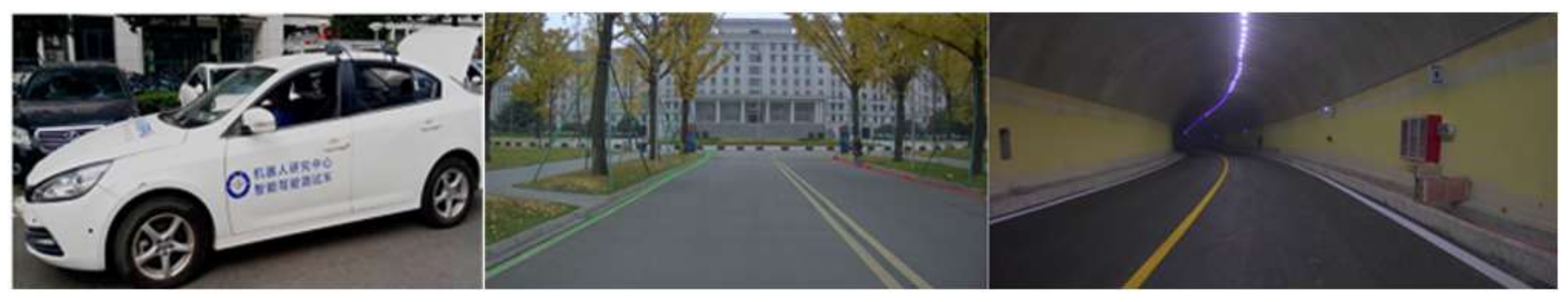
4. Experimental Verification
The platform was modified from the Junipai A70E electric vehicle, and the body was loaded with sensors such as IMU, GNSS and a monocular camera. The IMU sensor adopts MEMS products from Xsens, and the GNSS receiver adopts Huace P3 series products, and adopts the centimeter-level positioning service of Thousand Seek. Further, unmanned experiments were carried out on the Qingshuihe campus of the University of Electronic Science and Technology of China and the Longchi Tunnel. As shown in
Table 1.
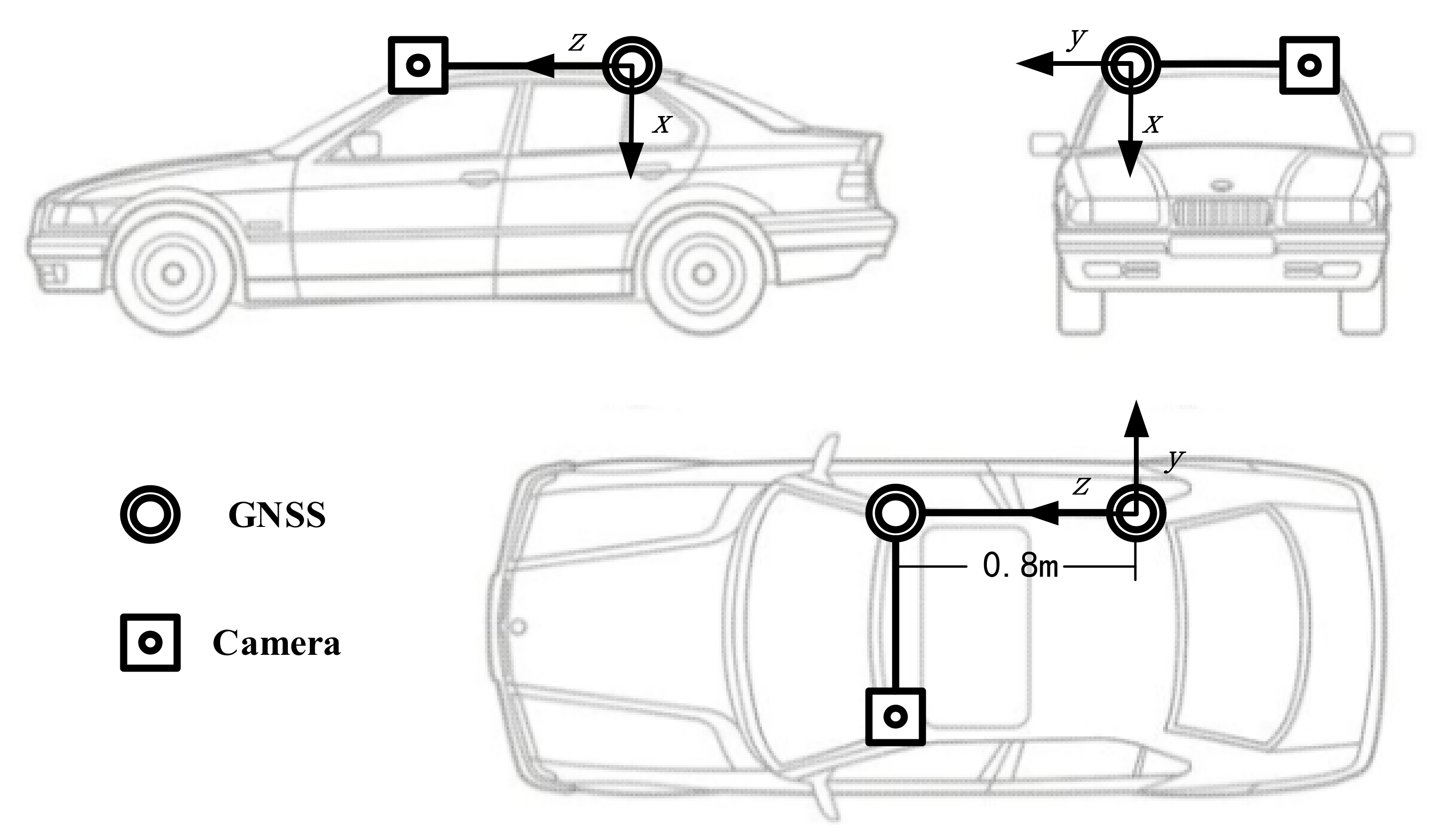
In the experiment, the monocular camera + IMU sensor installed on the roof was used to complete the SLAM system. The body has sensors such as GNSS [
24], IMU, and a camera. The GNSS dual-antenna device applied in the paper is used for true value positioning and orientation in unmanned driving experiments. Due to the dual antennas used, only the yaw angle and pitch angle of the vehicle can be calculated during orientation, but the roll angle cannot be calculated. Considering that the change of the roll angle of the vehicle body is small, it can be ignored in the actual application process. Most of the poses collected by GNSS represent the current position of the vehicle, so the GNSS antenna is required to be installed as parallel to the vehicle as possible.
Figure 6 and
Figure 7 below shows the relative positional relationship between the sensors fixed on the roof.
To evaluate the algorithm performance, an experimental analysis was performed. The work of map structuring can be stored in the map by the data collection vehicle and processed and obtained. It can also be completed by querying and interpolating the latitude and longitude on the Baidu map. Due to the basic deviation of the network map, the map data can be collected at the location with GNSS alignment.
The experimental data are that the data acquisition vehicle runs in the campus environment and the lane line area in the Longchi tunnel environment. This collects images and GNSS data. In order to judge the accuracy and performance of the algorithm, the true value data of the lane line position are needed. In this paper, the true value data of the lane line position were collected by a special trajectory acquisition vehicle. After the data were collected, the image data were used as the input of the algorithm, and the data collected by GNSS were used as the real value to evaluate the performance index of the algorithm. In the tunnel of the Longchi scene, there is a lack of real positioning value. This paper used the processed latitude and longitude interpolation results in the map as the real value, and fused the output positioning results and map data for trajectory error calculation.
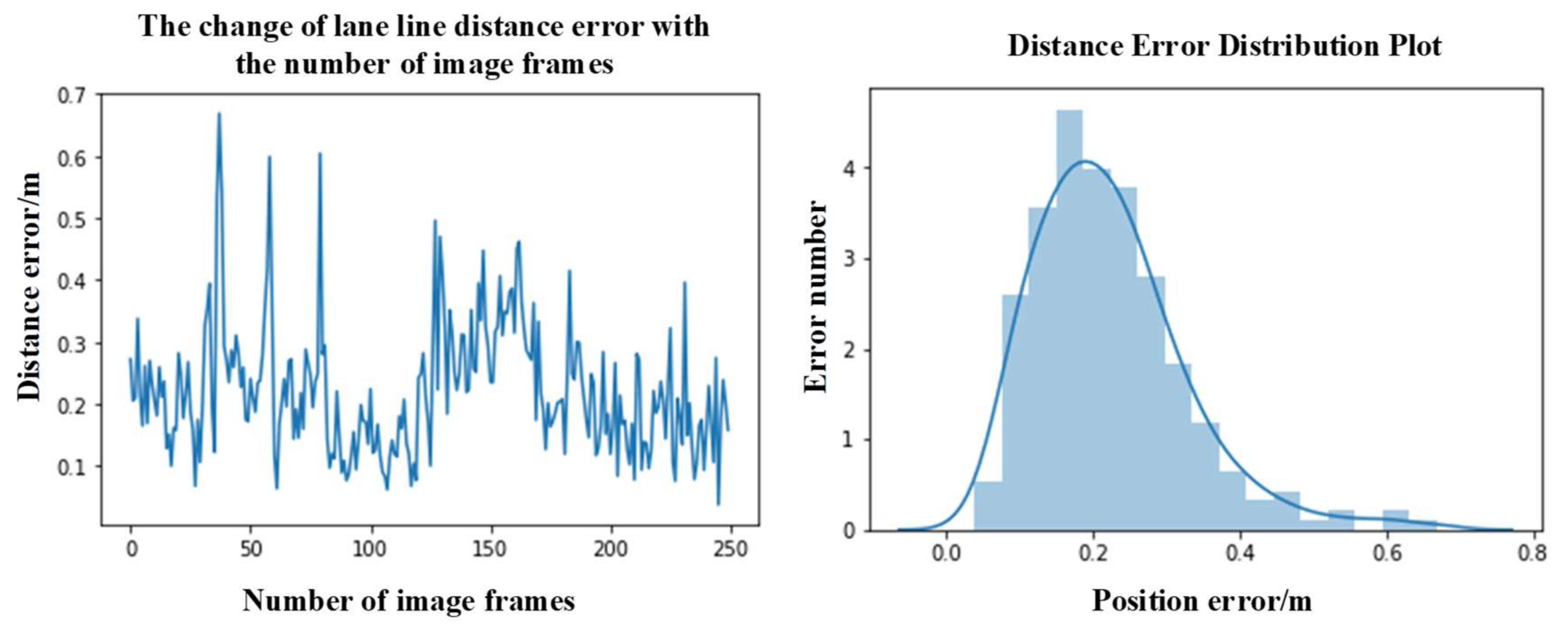
4.1. Experiment Results of Lane Line Positioning
In this paper, the monocular camera was used to calculate the relative position of the left and right lane lines, and the lane line positioning was determined. The true value was obtained by the data acquisition vehicle. The monocular camera positioning results of the lane line itself are as follows.
The error of distance
D has no obvious change with the number of frames, and the overall error is relatively stable. According to a statistical analysis of all the error data, as shown in the right of
Figure 8 above, the error distribution conforms to a skewed normal distribution, and most of the error distribution is within 0.3 m. The reliability of the vehicle position assumption used in this paper is generally stable.
4.2. Campus Scene Localization Experiment Results
This experiment was carried out in the campus area. The real map lane value was obtained by the data acquisition car driving along the lane, and it can be considered that there is no map lane information error. GNSS was used as the true value of the data to calculate the original SLAM method, the SLAM algorithm with relocation information, and the positioning results of lane line positioning at this time, and to compare them with the true value of GNSS. The positioning results are as follows.
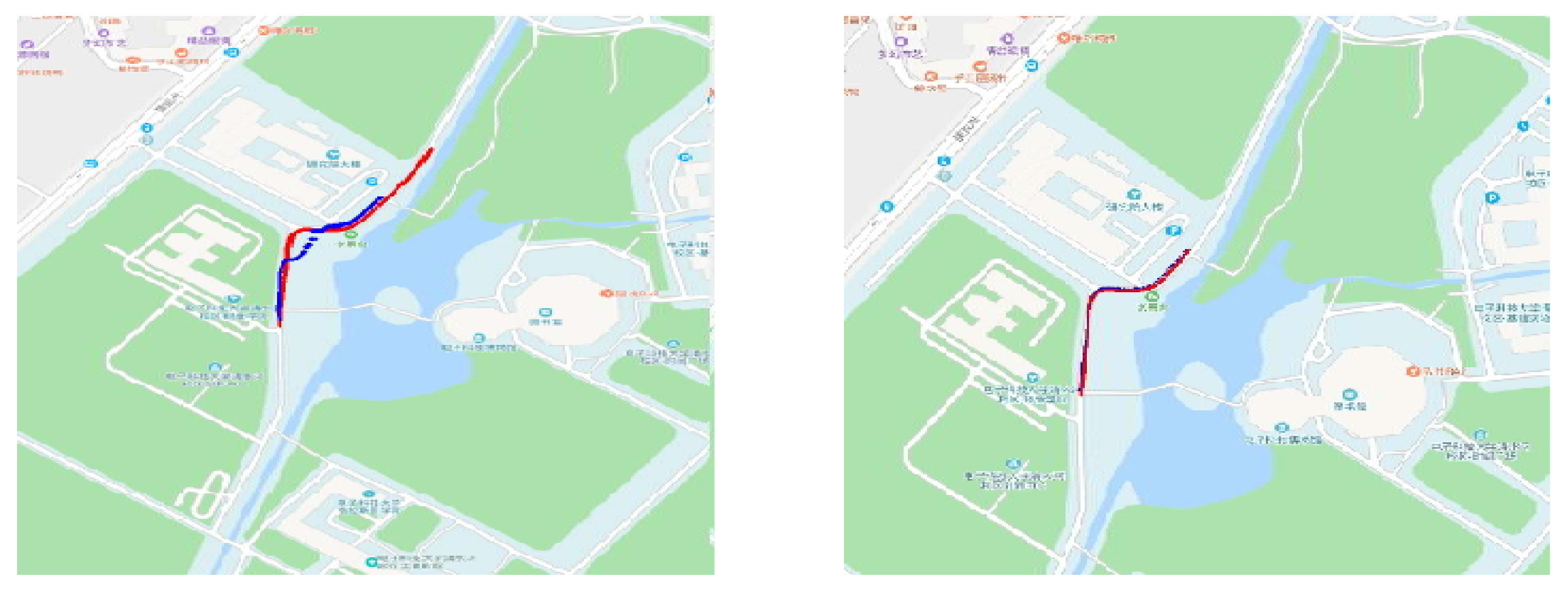
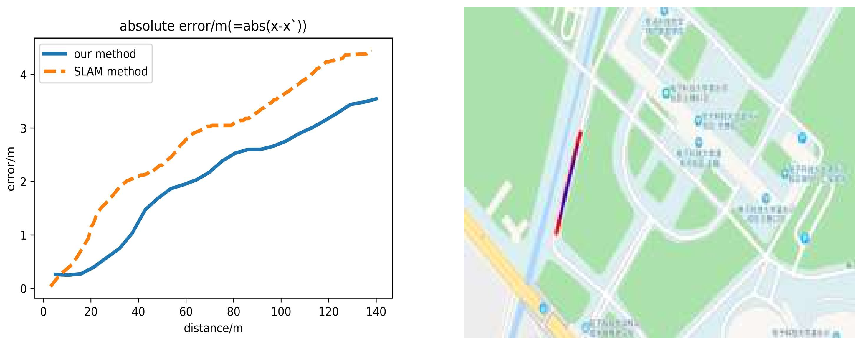
As shown in
Figure 9, the two lines represent the true value of GNSS and the result obtained by the original SLAM algorithm. Here, the algorithm adopts the VINS-Mono algorithm, and the positioning result is displayed on the map after the coordinate system transformation. The true value of the map is displayed. It can clearly be seen from
Figure 9 that the effect of the algorithm in this paper is better than the original SLAM method in practical application, and its positioning results basically coincide with the true value. It has a great influence, so the experiment is divided into two motion states of straight line and non-pure straight line.
When the lane is not a pure straight road, that is, the road has a radian, the
Q matrix in the equation can be updated to obtain an accurate estimate of the position, and the vehicle trajectory and the road trajectory can be fused by adjusting the coefficient. The results of the positioning experiment and the schematic diagram are shown in
Figure 10.
In detours, the divergence of SLAM positioning results is better limited, the cumulative error is eliminated, and the positioning results of <1 m are obtained in gentle detours, and the effect is good.
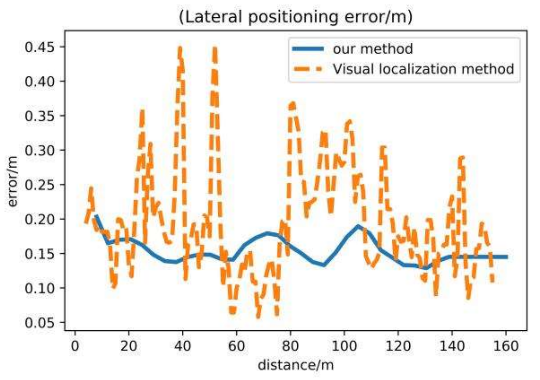
As shown in
Figure 11, In the straight-line experiment, since the lane line positioning information does not change greatly, the state quantity of the positioning cannot be corrected by observation, and the fusion positioning result at this time is expressed as the output lag of SLAM. The method proposed in this paper relies on the effective map information. When the pure linear motion has a lack of effective observation, the error cannot be corrected.
However, in pure linear motion, although the error cannot be corrected by map information, the lateral positioning accuracy can still meet the needs of vehicle navigation. The results of lateral local positioning information are shown in
Figure 12.
As shown in
Figure 12, the local positioning error does not exceed 0.3 m in most cases. When moving in a straight line, the lane can be cruised through local positioning. When encountering a detour, due to the fast-converging observation method set in the previous article, it can quickly converge to the location where it is located.
To summarize, the algorithm proposed in this paper has a good positioning effect on non-pure straight roads, and the positioning accuracy is greatly improved, while in pure straight line motion, the algorithm accuracy is less improved, but the results of lateral local positioning meet the requirements of unmanned driving. As shown in
Table 2, the numerical analysis is as follows:
As shown in the table above, in the data experiment of detours, the localization algorithm after integrating map information achieved good results, the global positioning accuracy improved by more than 70%, and the local positioning was also significantly improved, which is more suitable for behavior scenarios involving unmanned positioning use.
4.3. Experiments Results in Closed Loop Path
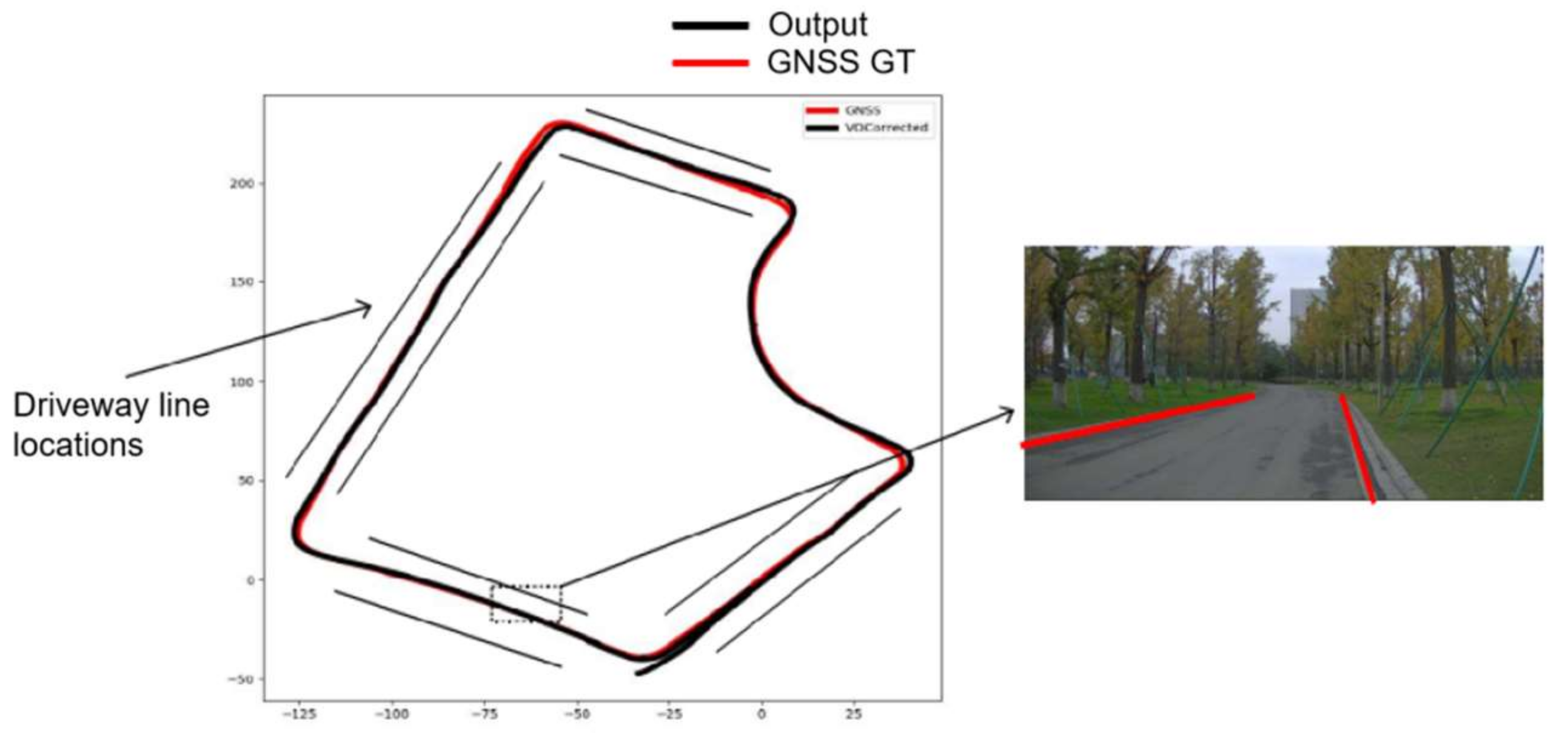
As shown in
Figure 13, The data set was collected at the south gate of the University of Electronic Science and Technology for the location experiment. The data were collected using the same experimental platform as in the previous section. The platform was equipped with GNSS terminals, cameras and other equipment to collect the dataset in data collection vehicle mode to obtain image data and GNSS position data during vehicle operation.
Compared to the original slam algorithm, our algorithm error is greatly improved, and the lane line positioning algorithm is able to constrain the lateral position of the vehicle relative to the lane line with good accuracy, eliminating most of the vehicle lateral position error. As shown in
Table 3.
4.4. Longchi Tunnel Scene Location Experiment Results
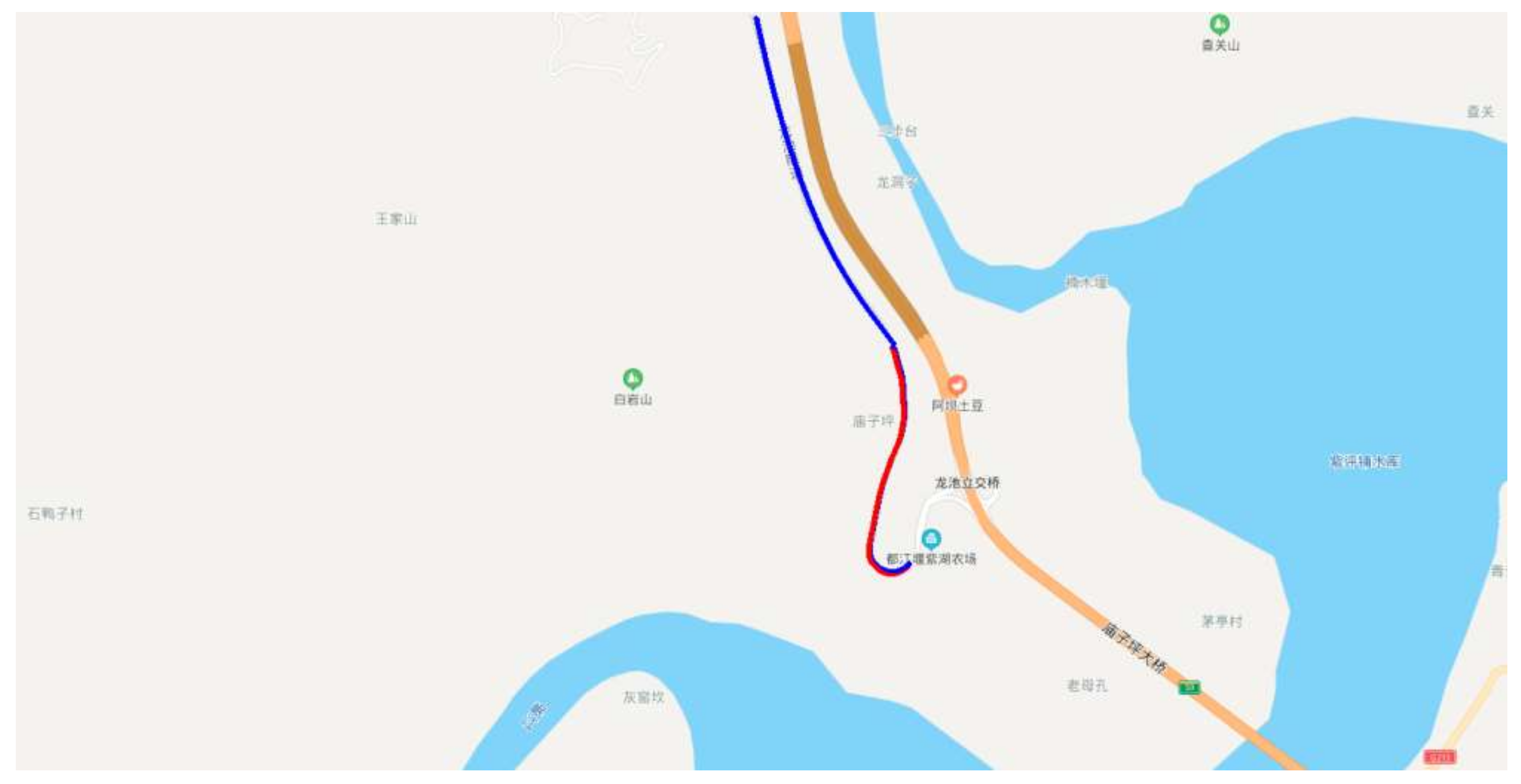
The method proposed in this paper can still achieve good positioning results in tunnels without GNSS. A 1 km unmanned tunnel experiment was carried out in Longchi Tunnel, Dujiangyan City, Sichuan Province. The tunnel is well-lit and the lane lines are clear. In the tunnel scene, the unmanned vehicle has completed the navigation function, and its driving trajectory is as follows
Figure 14:
In the experiment, since there is no GNSS true value in the tunnel, the above error calculation cannot be performed. In this paper, the comparison between the driving trajectory and the trajectory of the tunnel itself was used for calculation. The specific method adopts the assumption of uniform speed to calculate the distance between the driving trajectory point and the road trajectory point.
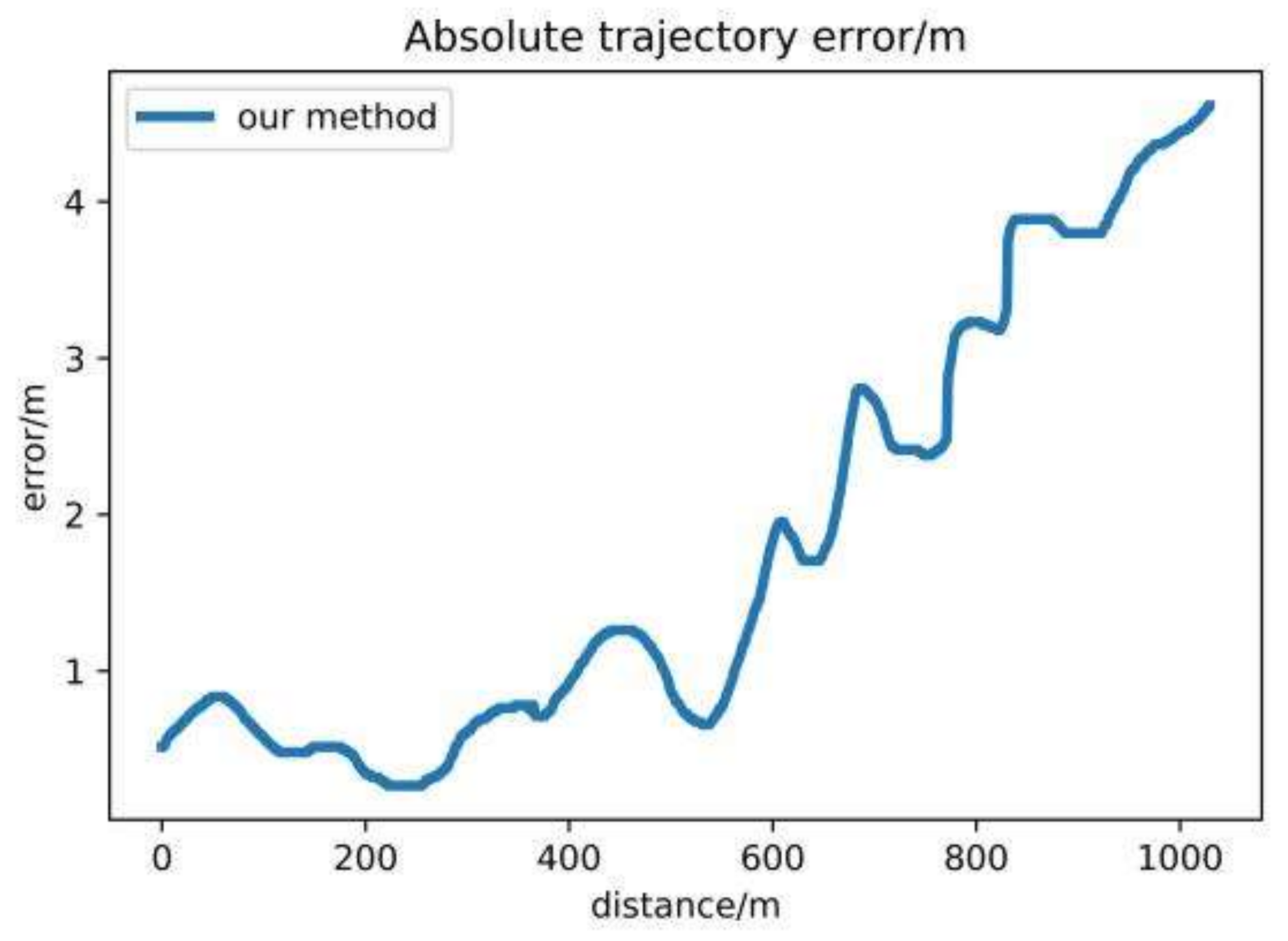
It can be seen from
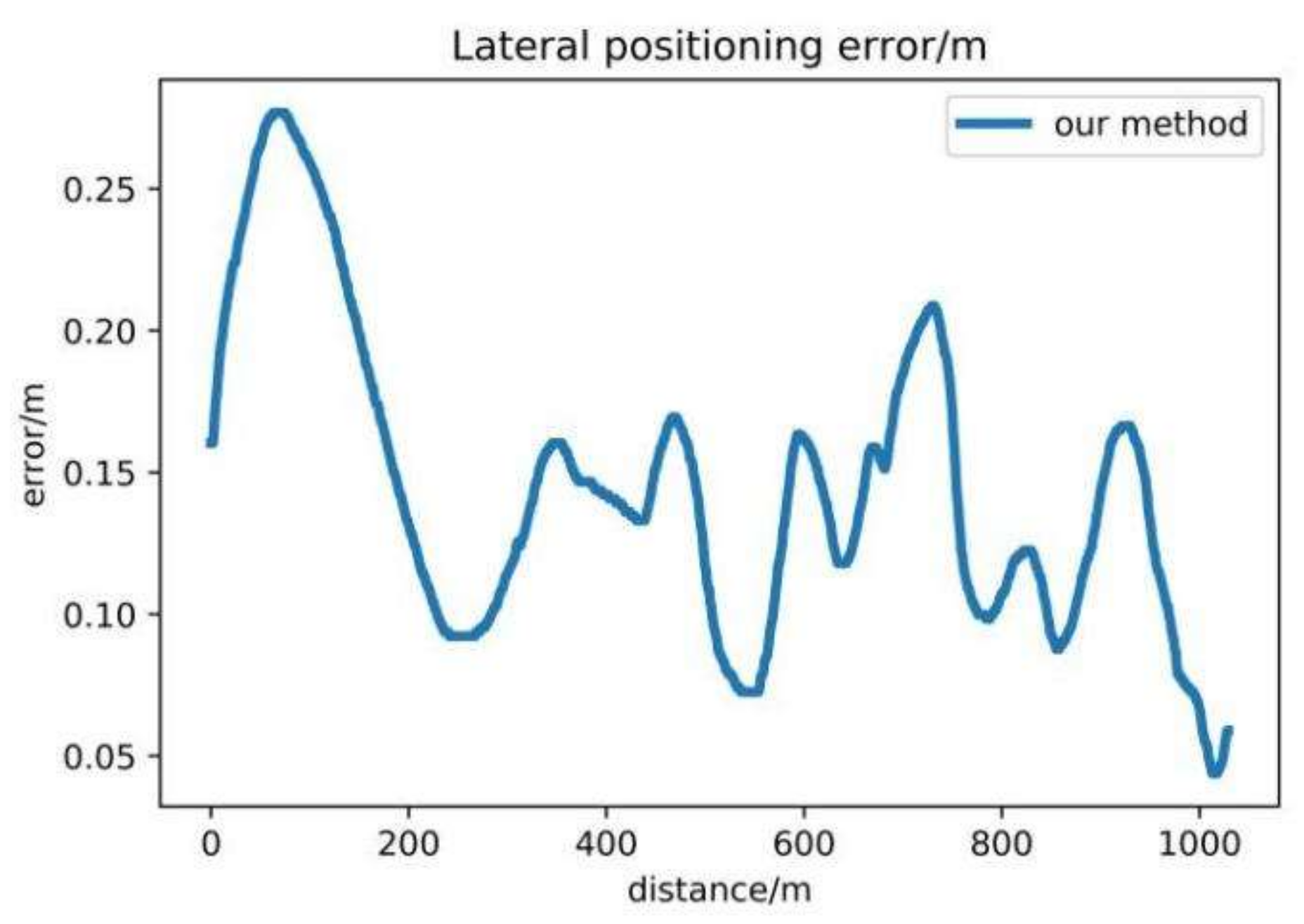
Figure 15 above that the positioning results are more accurate in the radian part of the tunnel. Due to the uniform speed assumption model, the results have a certain gap with the real results, but it can still clearly reflect the positioning of the method in this paper under certain changes in road observations. The effect is improved. The angle change in the second half of the tunnel is small, the observation and correction effect of the map is small, and the accumulated error is difficult to eliminate. After driving 600 m, the error reached m level, but the lateral local positioning results are still relatively stable. The distance between the driving trajectory and the road trajectory is calculated in the direction as the lateral positioning error.
As shown in
Figure 16, the lateral error positioning errors are all less than 0.35 m, and the initial positioning error is the error of the lane line positioning itself. Through the recalculation of the fusion positioning results, the positioning accuracy has been greatly improved and can be stabilized around 15 cm, which is sufficient. The unmanned vehicle completes the positioning and navigation in the fixed tunnel.
It is worth noting that since there is no true value in the tunnel itself, the above two calculation methods are an approximate analysis, and the error between the true value and the positioning result is theoretically close to this method. Since the vehicle trajectory is smooth, the tunnel angle changes less, and the distance between the tangential directions and the actual point is less.
Through the above analysis, there are no GNSS scenarios such as tunnels. After the fusion of map lane information and the SLAM positioning method, the positioning accuracy has been greatly improved, and it has a good effect in global and local positioning, as well as better stability. The algorithm proposed in this paper can effectively complete the navigation under local positioning. Compared with the SLAM algorithm itself, the global positioning accuracy is greatly improved, which has great advantages for actual navigation.
This paper gives a summary of the following rules:
When the method in this paper moves in a pure straight line, the effect of the fusion positioning is the worst, which is basically only the lag of the SLAM output result.
The fusion of the method in this paper can effectively suppress the divergence of positioning errors and ensure the positioning requirements of unmanned vehicles. The lateral positioning results are always stable within 20 cm, which is sufficient for unmanned navigation in the local coordinate system.
Due to the continuity of the observation equation, the radius of curvature is small, but the position error with frequent changes is the smallest, which can be below the meter level.
5. Summary and Outlook
In this paper, by integrating SLAM positioning and map information, combined with the local stability and non-divergence of lane line positioning, and the globality and continuity of SLAM, a prior map of lane lines based on directed graphs is established to solve the problem of unmanned vehicle positioning. There is a lack of correlation between local positioning and global positioning, and the positioning results are not robust enough, especially in the case of GNSS failure, providing good local positioning information to ensure the realization of the navigation function. While preventing the divergence of global information, the positioning application of unmanned vehicles have a certain contribution. At the same time, the positioning method described in this paper can be applied to more scenes, such as semantic map information, the image information of known positioning, etc. By establishing observation equations and judging and adjusting one’s own position, the accuracy of positioning can be increased further. The method proposed in this paper has practical application significance in universal map construction and localization. However, it is highly dependent on the observability of road information, and the fusion effect is limited when the road is a pure linear motion, which needs further research.
Driverless positioning technology is developing rapidly, and more sensors and algorithms are being proposed. Sensors such as millimeter wave radar, ultrasonic radar and infrared are all important in driverless positioning technology. SLAM systems are one of the important methods of multi-source sensor fusion, and we believe that the combined application of deep learning technology and SLAM will be an important method for future driverless capability.


