Robust Estimation in Continuous–Discrete Cubature Kalman Filters for Bearings-Only Tracking

Abstract

The model of bearings-only tracking is generally described by discrete–discrete filtering systems. Discrete robust methods are also frequently used to address measurement uncertainty problems in bearings-only tracking. The recently popular continuous–discrete filtering system considers the state model of the target to be continuous in time, and is more suitable for bearings-only tracking because of its higher mathematical solution accuracy. However, the sufficient evaluation of robust methods in continuous–discrete systems is not available. In addition, in the different continuous–discrete measurement environments, the choice of a robust algorithm also needs to be discussed. To fill this gap, this paper firstly establishes the continuous–discrete target tracking model, and then evaluates the performance of proposed robust square-root continuous–discrete cubature Kalman filter algorithms in the measurement of uncertainty problems. From the simulation results, the robust square-root continuous–discrete maximum correntropy cubature Kalman filter algorithm and the variational Bayesian square-root continuous–discrete cubature Kalman filter algorithm have better environmental adaptability, which provides a promising means for solving continuous–discrete robust problems.

1. Introduction

Bearings-only tracking [1,2] uses a sequence of angle measurements to estimate the state (position and velocity) of the target and has universal applications in the field of navigation, especially in passive target tracking. For the system model of bearings-only tracking, the target state is generally built as the discrete time model for convenience. In addition, the angle measurement information for the target is discrete time. This is called the discrete–discrete time system model. However, considering the actual situation of target tracking, the target state is continuous in nature, and the measurement is discrete time. Such a system model is called the continuous–discrete time system [1]. Compared with the discrete–discrete system model, the continuous–discrete system model is closer to the real situation, and its solutions have more advantages, such as high accuracy [3].

Based on the continuous–discrete time system, continuous–discrete filtering, whose model is based on the covariance matrix of random errors, can be established. In [4], the cubature criterion was introduced into the continuous–discrete time system, and the continuous–discrete cubature Kalman filter (CD-CKF) algorithm was obtained. It uses stochastic differential equations (SDEs) to describe the continuous-time target state model, and the accuracy of the SDE solution greatly affects the filtering performance. In [5], Crouse summarized the Euler-Maruyama method based on 0.5 order and the Itô-Taylor method, which were proven to have acceptable accuracy. In order to further improve the accuracy of state estimation, high-order numerical approximation methods are used to deal with stochastic differential equations. In [6], Crouse described the continuous-time model as the form of its expectation and covariance and then solved the time prediction problem of the continuous model. In [7], the nested implicit Runge-Kutta method was used for the continuous–discrete extended Kalman filter (CD-EKF), and the corresponding application in CD-CKF was discussed in [8]. Subsequently, adaptive methods were proposed. In [9], Kulikova et al. used adaptive step size to further improve the accuracy. The adaptive feedback strategy [10] reduced the impact of unpredictable errors in the prediction step by means of covariance adjustment; thus, the performance and efficiency were both improved.

In the actual measurement environment, harsh conditions such as signal interference will cause non-Gaussian noise [11,12] or outliers to appear. If they are not dealt with, the Gaussian-assumed filters will be inaccurate or even divergent. For this measurement uncertainty problem, various robust methods [13] are proposed for the discrete–discrete time filtering systems. As a method of modification, robust methods aim to improve robustness in the presence of outliers in the data. For instance, the Huber’s M-estimation method [14,15] used the robust cost function to reduce the weight of abnormal data. It is widely used and has proven effective in filtering problems [16]. Wu et al. [17,18] proposed a more practical robust CKF algorithm based on generalized M-estimation without the experience threshold of the weight function and statistical characteristics information of outliers. In [19], Särkkä dealt with the time-varying noise with the variational Bayes criterion in the case of unknown noise covariance. In [20,21,22], the maximum correntropy criterion (MCC) was introduced into discrete–discrete filtering systems. The correntropy can utilize the higher-order information of the measurements instead of the second-order moment information of the minimum mean square error criterion, which is more suitable for non-Gaussian systems in the presences of non-Gaussian noise.

The above robust methods are successfully used in the discrete–discrete time systems, but sufficient evaluation of the continuous–discrete time systems is not available. Moreover, how to balance the accuracy and robust performance of the continuous–discrete filtering algorithms is of great significance. Therefore, this paper proposes the square-root continuous–discrete cubature Kalman filter (SRCD-CKF) with Huber’s method, maximum correntropy criterion, and variational Bayesian criterion, and analyzes their filtering performance in the measurement of uncertainty problems. The CD-CKF is chosen because it is derivative-free and generally more accurate than the CD-EKF. Additionally, compared with the continuous–discrete unscented Kalman filter (CD-UKF), CD-CKF has the smaller computational burden. The square-root technique can also improve the stability of the filter. Compared with the proposed robust algorithms, the robust square-root continuous–discrete maximum correntropy cubature Kalman filter (RSRCD-MCCKF) algorithm and the variational Bayesian square-root continuous–discrete cubature Kalman filter (VBSRCD-CKF) algorithm have higher accuracy and stronger robustness.

To sum up, in this paper, the robust estimation methods based on a continuous–discrete system are proposed to solve the problem of sufficient evaluation of continuous–discrete robust algorithms. Compared with the discrete–discrete filtering system, considering the continuous–discrete filtering system can effectively ensure the accuracy of bearings-only tracking, while the robust methods are used to improve the robustness of the tracking. From the perspective of improving accuracy and robustness, the proposed algorithms have excellent performance in continuous–discrete systems. Another contribution is that the article compares the performance of the algorithms in different continuous–discrete measurement environments, fully considering the environmental adaptability of the algorithms.

The structure of the rest of the article is as follows: Section 2 reviews the target tracking model of the continuous–discrete system and the algorithm of SRCD-CKF, Section 3 proposes the robust SRCD-CKF algorithms with Huber’s method, the RSRCD-MCCKF algorithm, and the VBSRCD-CKF algorithm, Section 4 shows the results of the simulation, and Section 5 summarizes the main work of this paper.

2. Continuous–Discrete System Model and Square-Root Continuous–Discrete Cubature Kalman Filter Algorithm for Target Tracking

2.1. Continuous–Discrete System Model

In a continuous–discrete target tracking system, the target state model is continuous time, and the measurement model is discrete time. Considering the random disturbance, the continuous-time target state model can be described as the following stochastic differential equation form [1]:

$$dx(t)=f(x(t),t)\mathit{dt}+\sqrt{Q}dw(t),$$

(1)

where $x(t)$ is the n-dimensional state vector, $f$ is known as the drift function, $w(t)$ is the zero-mean Gaussian white-noise process, and $Q$ represents the covariance matrix of the zero-mean Gaussian white-noise process.

In order to deal with the continuous time model, the target model of the continuous–discrete system can be described by the moment differential equations (MDEs) [9], which are shown as

$$\frac{d\widehat{x}(t)}{\mathit{dt}}=F(\widehat{x}(t)),$$

(2)

$$\frac{dP(t)}{\mathit{dt}}=J(\widehat{x}(t))P(t)+P(t)J^{\mathrm{T}}(\widehat{x}(t))+Q,$$

(3)

where $\widehat{x}(t)$ is the expectation of $x(t)$ at time t, $P(t)$ represents the error covariance matrix at time t, $F(\widehat{x}(t))$ is the state equation of the system, and the Jacobian matrix of $F(\widehat{x}(t))$ is $J(\widehat{x}(t))$, that is, $J(\widehat{x}(t))=\partial F(\widehat{x}(t))/\partial \widehat{x}(t)$.

The discrete time measurement model is

$$z_k=h\left(x_k,k\right)+r_k,$$

(4)

where $z_k$ is the actual observation value, $h$ is the observation function, and $r_k$ is the observation noise, which refers to Gaussian or non-Gaussian noise. The specific noise form of $r_k$ is defined by the measurement scenario, and its covariance matrix is $R_k^{}$. Here, k refers to discrete time measurement points.

2.2. Square-Root Continuous–Discrete Cubature Kalman Filter Algorithm

In order to ensure the positive definiteness and symmetry of the error covariance matrix, the square-root continuous–discrete cubature Kalman filter is introduced here. Similar to the typical CKF method, the continuous–discrete time system is combined with the cubature criterion, which is also divided into two steps: time update and measurement update.

In the SRCD-CKF algorithm, the state cubature points can be defined as [23]

$$X_i(t)=S(t){\xi }_i+\widehat{x}(t),$$

(5)

where $S(t)$ is the lower triangular matrix of the covariance matrix, satisfying $P(t)=S(t)S^{\mathrm{T}}(t)$, and ${\xi }_i$ is the cubature point set, which is defined as

$${\xi }_i(t)=\left\{\begin{array}{cc}\sqrt{n}{\eta }_i& i=1,\cdots ,n\\ \sqrt{n}{\eta }_{i-n}& i=n+1,\cdots ,2n\end{array}\right.$$

(6)

where ${\eta }_i$ is the i-th coordinate column-vector in ${ℝ}^n$.

Based on the cubature criterion, its expectation and covariance can be re-expressed as

$$\frac{d\widehat{x}(t)}{\mathit{dt}}=F(X(t))\epsilon ,$$

(7)

$$\frac{dP(t)}{\mathit{dt}}=X(t)W{F}^{\mathrm{T}}(X(t))+F(X(t))X^{\mathrm{T}}(t)+Q(t).$$

(8)

The parameters of $\epsilon$ and $W$ are defined as follows:

$$\left\{\begin{array}{c}\epsilon =\frac{\mathbf{1}}{2n}\\ W=(I_{2n}-{\mathbf{1}}^{\mathrm{T}}\otimes \epsilon )\mathrm{diag}\left[1/(2n),\cdots ,1/(2n)\right]{(I_{2n}-{\mathbf{1}}^{\mathrm{T}}\otimes \epsilon )}^{\mathrm{T}}\end{array}\right.,$$

(9)

where $I_{2n}$ represents a unit matrix with a dimension of 2n, $\mathbf{1}$ is a unit column vector, and $\otimes$ represents the Kronecker tensor.

For the calculation of covariance propagation, the square-root covariance calculation method proposed in [24] is used. Meanwhile, the high-order numerical approximation method is used to deal with the problem:

$$\frac{dS(t)}{\mathit{dt}}=S(t)\Phi (B),$$

(10)

$$\Phi (B)=\left\{\begin{array}{cc}{B}_{i,j} & \mathit{if} i>j\\ \frac{1}{2}{B}_{i,j} & \mathit{if} i=j\\ 0 & \mathit{if} i<j\end{array}\right.,$$

(11)

where $B_{i,j}$ is the element in the i-th row and j-th column of $\Phi (B)$. The definition of $B(t)$ matrix is

$$B(t)=S^{-1}(t)\left[X(t)W{F}^{\mathrm{T}}(X(t))\right.+\left.F(X(t))X^{\mathrm{T}}(t)+Q(t)\right]S^{-\mathrm{T}}(t).$$

(12)

Based on this, the predicted state cubature point $X_i^{*}(t)$ can be obtained. The specific SRCD-CKF Algorithm 1 is as follows:

Algorithm 1: SRCD-CKF.

Time update  Step 1 Expectation and covariance matrix initialization: $\widehat{x}\left(t_k\right)={\widehat{x}}_{k-1\left|k-1\right.}$, $P\left(t_k\right)=P_{k-1\left|k-1\right.}$.  Step 2.1 Covariance decomposition: $P(t_k)=S(t_k)S^{\mathrm{T}}(t_k)$.  Step 2.2 Calculate the state cubature point: $X_i(t_k)=S(t_k){\xi }_i+\widehat{x}(t_k)$.  Step 2.3 State cubature point propagation: $\left\{\begin{array}{l}\widehat{x}\prime (t)=F(X(t))\epsilon \\ \\ S\prime (t)=S(t)\Phi (B(t))\end{array}\right.$.  Step 2.4 Calculate the state prediction value: ${\widehat{x}}_{k\left|k-1\right.}=\left(X_1^{*}(t_k)+\cdots +X_{2n}^{*}(t_k)\right)/2n$.  Step 2.5 Calculate the predicted square-root covariance:

$S(t_k)=\left[\begin{array}{cccc}{S}_1(t_k)& S_2(t_k)& \cdots & S_{2n}(t_k)\end{array}\right],$

$\mathrm{where}{S}_i(t_k)$$\mathrm{represents}a\sin \mathrm{gle}\mathrm{column}\mathrm{vector},S_i(t_k)=\left(X_i^{*}(t_k)-{\widehat{x}}_{k\left|k-1\right.}\right)/\sqrt{\mathrm{n}}$.  Measurement update  Step 3.1 Calculate the state cubature point: $S_{k|k-1}^{}=S(t_k)$, $X_{i,k\left|k-1\right.}=S_{k|k-1}^{}{\xi }_i+{\widehat{x}}_{k\left|k-1\right.}$.  Step 3.2 Measure the spread of cubature points: $Z_{i,k\left|k-1\right.}=h(X_{i,k\left|k-1\right.},k)$.  Step 3.3 Calculate the predicted value of the measurement: ${\widehat{z}}_{k\left|k-1\right.}=\frac{1}{2n}{\displaystyle \sum _{i=1}^{2n}{Z}_{i,k\left|k-1\right.}}$.  Step 3.4 Construct the measurement weighted center matrix:

$Z_{k\left|k-1\right.}=\frac{1}{\sqrt{2n}}\left[Z_{1,k\left|k-1\right.}-{\widehat{z}}_{k\left|k-1\right.} ,\cdots , Z_{2n,k\left|k-1\right.}-{\widehat{z}}_{k\left|k-1\right.}\right].$

Step 3.5 Calculate the innovation covariance matrix: $P_{\mathit{zz},k\left|k-1\right.}=Z_{k\left|k-1\right.}^{}{Z}_{k\left|k-1\right.}^T+R_k^{}$.  Step 3.6 Construct the state weighted center matrix:

$X_{k\left|k-1\right.}=\frac{1}{\sqrt{2n}}\left[X_{1,k\left|k-1\right.}-{\widehat{x}}_{k\left|k-1\right.} ,\cdots , X_{2n,k\left|k-1\right.}-{\widehat{x}}_{k\left|k-1\right.}\right].$

Step 3.7 Calculate the cross covariance matrix: $P_{\mathit{xz},k\left|k-1\right.}^{}=X_{k\left|k-1\right.}^{}{Z}_{k\left|k-1\right.}^{\mathrm{T}}$.  Step 3.8 The continuous–discrete cubature gain is: $K_k^{}=P_{\mathit{xz},k|k-1}^{}{P}_{\mathit{zz},k|k-1}^{-1}$.  Step 3.9 Calculate the state estimate: ${\widehat{x}}^{}{}_{k\left|k\right.}={\widehat{x}}_{k\left|k-1\right.}+K_k^{}(z_k-{\widehat{z}}_{k\left|k-1\right.})$.  Step 3.10 Update the covariance matrix: $P_{k|k}^{}=P_{k|k-1}^{}-K_k^{}{P}_{zz,k|k-1}{K}_k^{\mathrm{T}}$.

Remark 1.

The above method gives the square root form of the prediction covariance and uses it for the measurement update process. The algorithm has effectively guaranteed the stability of the filtering. At the same time, a more thorough square-root version is also available.

Here we redefine the cross-covariance matrix $P_{\mathit{xz},k\left|k-1\right.}^{}$, the innovations covariance square-root $R_{e,k}^{1/2}$, and the filtering covariance square-root $S_{k|k}^{}$ by QR decomposition:

$$\mathrm{qr}\left[\begin{array}{cc}{Z}_{k\left|k-1\right.}& R_k^{1/2}\\ X_{k\left|k-1\right.}& 0\end{array}\right]=\left[\begin{array}{cc}{R}_{e,k}^{1/2}& 0\\ P_{\mathit{xz},k\left|k-1\right.}^{}& S_{k|k}^{}\end{array}\right],$$

(13)

where $0$ is the zero-block of a proper size, $R_k^{1/2}$ is the measurement noise covariance square-root obtained by Cholesky factorization, and $R_{e,k}^{1/2}$ and $S_{k|k}^{}$ are lower triangular matrices.

On this basis, we can obtain the update state and covariance. In addition, the robust estimation methods under this square-root version can be obtained according to our idea.

3. Robust Square-Root Continuous–Discrete Cubature Kalman Filter Algorithms

3.1. Robust SRCD-CKF with Huber’s Method

The robust SRCD-CKF algorithms are used to correct the abnormal measurements. Huber’s method uses the robust cost function to reduce the weight of abnormal data. Among them, the most common weight reduction functions are the two-stage weight function based on Huber and the three-stage weight function based on p-Huber. The Huber weight function usually includes two parts. This means that the measurement data are divided into normal data and abnormal data. When the absolute value of the standardized residual exceeds the critical value, the data are considered abnormal and the weight is reduced.

$${\overline{\mathsf{\mu }}}_k=\left\{\begin{array}{l}1,\left|{\tilde{\lambda }}_{\mathrm{b}}\right|<\mathrm{c}\\ \\ \mathrm{c}/\left|{\tilde{\lambda }}_{\mathrm{b}}\right|,\left|{\tilde{\lambda }}_{\mathrm{b}}\right|\ge \mathrm{c}\end{array}\right.,$$

(14)

where $\left|{\tilde{\lambda }}_{\mathrm{b}}\right|$ is the absolute value of the standardized residuals, and c is the critical value of abnormal error discrimination. The Huber robust square-root continuous–discrete cubature Kalman filter (HRSRCD-CKF) Algorithm 2 is as follows:

Algorithm 2: HRSRCD-CKF.

Step 1 Repeat Step 1 of the SRCD-CKF algorithm.  Steps 2.1–3.7 are equivalent to Steps 2.1–3.7 of the SRCD-CKF algorithm.  Step 3.8 The innovation covariance matrix is redefined: ${\overline{P}}_{\mathit{zz},k\left|k-1\right.}=Z_{k\left|k-1\right.}^{}{Z}_{k\left|k-1\right.}^{\mathrm{T}}+{\overline{\mu }}_k^{-1}{R}_k^{}$.  Step 3.9–3.11 are equivalent to Steps 3.8–3.10 of the SRCD-CKF algorithm.

The weight function based on the Mahalanobis distance is also called the p-Huber three-stage weight function. Compared with the Huber function, the p-Huber function uses the $\mathsf{\alpha }$ quantile of the chi-square distribution to adjust the critical value of abnormal error discrimination, which is more reasonable than the empirical value. The discriminant value is defined as follows:

$$d_k={\mathrm{M}}_k^2={(z_k-{\widehat{z}}_{k\left|k-1\right.})}^{\mathrm{T}}{\left({\mathit{P}}_{zz,k|k-1}\right)}^{-1}(z_k-{\widehat{z}}_{k\left|k-1\right.}).$$

(15)

In Equation (15), ${\mathrm{M}}_k=\sqrt{{(z_k-{\widehat{z}}_{k\left|k-1\right.})}^{\mathrm{T}}{\left({\mathit{P}}_{zz,k|k-1}\right)}^{-1}(z_k-{\widehat{z}}_{k\left|k-1\right.})}$ is the Mahalanobis distance. The new three-stage weight function is

$${\overline{\mathsf{\mu }}}_k=\left\{\begin{array}{l}1,d_k<{\chi }_{\mathsf{\alpha }1}\\ \\ \sqrt{{\chi }_{\mathsf{\alpha }1}/d_k},{\chi }_{\mathsf{\alpha }1}\le d_k<\\ \\ 0,d_k\ge {\chi }_{\mathsf{\alpha }2}\end{array}\right.{\chi }_{\mathsf{\alpha }2},$$

(16)

where ${\chi }_{\mathsf{\alpha }}$ is the quantile of the chi-square distribution. When $d_k$ exceeds ${\chi }_{\mathsf{\alpha }1}$, it is considered that there is an outlier in the measurement, and its weight needs to be reduced. At the same time, in order to further eliminate the influence of large outliers, when $d_k\ge {\chi }_{\mathsf{\alpha }2}$, they will be eliminated. The M-estimation–based robust square-root continuous–discrete cubature Kalman filter (MRSRCD-CKF) Algorithm 3 is as follows:

Algorithm 3: MRSRCD-CKF.

Step 1 Repeat Step 1 of the SRCD-CKF algorithm.  Steps 2.1–3.7 are equivalent to Steps 2.1–3.7 of the SRCD-CKF algorithm.  Steps 3.8–3.11 are equivalent to Steps 3.8–3.11 of the HRSRCD-CKF algorithm, and ${\overline{\mathsf{\mu }}}_k$ is calculated by Equation (16).

3.2. RSRCD-MCCKF Algorithm Based on Maximum Correntropy Criterion

Correntropy is a new method used to measure the similarity between two random variables. Given the random variables X and Y, their joint probability density function is $F_{X,Y}\left(x,y\right)$. The correntropy can be defined as follows [22]:

$$V\left(X,Y\right)=E\left[\kappa \left(X,Y\right)\right]={\displaystyle \iint \kappa }\left(x,y\right)\mathrm{d}{F}_{X,Y}\left(x,y\right),$$

(17)

where $E\left[\cdot \right]$ is the mathematical expectation, and $\kappa \left(\cdot \right)$ is the Messer-type positive definite kernel function. In this paper, we select the Gaussian kernel as the kernel function of the correntropy, which is defined as follows:

$$\kappa \left(x,y\right)=G_{\mathsf{\sigma }}\left(e\right)=\exp \left(-\frac{e^2}{2{\mathsf{\sigma }}^2}\right),$$

(18)

where $e=x-y$, and $\mathsf{\sigma }>0$ is the kernel bandwidth of the kernel function.

In practice, the joint probability density function is usually difficult to obtain, and the data sampling points are also limited. Therefore, the correntropy can be estimated by the approach of T data sampling points:

$$\widehat{V}\left(X,Y\right)=\frac{1}{T}{\displaystyle \sum _{i=1}^T{G}_{\mathsf{\sigma }}\left(e\left(i\right)\right)}.$$

(19)

where $e\left(i\right)=x\left(i\right)-y\left(i\right)$, ${\left\{x\left(i\right),y\left(i\right)\right\}}_{i=1}^T$ represents the related sampling point sequence of the joint probability density function $F_{X,Y}\left(x,y\right)$. Expanding the Gaussian kernel function using the Taylor series, we can obtain

$$V\left(X,Y\right)={\displaystyle \sum _{n=0}^{\infty }\frac{{\left(-1\right)}^n}{2^n{\mathsf{\sigma }}^{2n}n!}}E\left[{\left(X-Y\right)}^{2n}\right].$$

(20)

It can be seen from Equation (20) that the correntropy information contains all the even-order moments of the random variable error X−Y. Therefore, as long as the appropriate kernel bandwidth is selected, higher-order information can be obtained. For the systems contaminated by noise, compared with the minimum mean square error criterion, the correntropy can be used to describe its statistical information.

On this basis, this paper introduces MCC into the continuous–discrete system. Firstly, ${\overline{H}}_k$ is defined as the pseudo-measurement matrix, ${\overline{R}}_k$ is the estimated covariance matrix of the observation noise, and their calculation methods are as follows:

$${\overline{H}}_k=P_{\mathit{xz},k\left|k-1\right.}^T{P}_{k\left|k-1\right.}^{-1},$$

(21)

$${\overline{R}}_k=P_{zz,k\left|k-1\right.}-{\overline{H}}_k{P}_{k\left|k-1\right.}{\overline{H}}_k^{\mathrm{T}}.$$

(22)

The cost function based on the MCC filtering can be defined by

$$J_{\mathrm{MCC}}=G_{\mathsf{\sigma }}\left({‖x_k-{\widehat{x}}_{k\left|k-\right.1}‖}_{P_{{}_{k\left|k-\right.1}}^{-1}}^2\right)+G_{\mathsf{\sigma }}\left({‖z_k-{\overline{H}}_k{x}_k-{\widehat{z}}_{k\left|k-1\right.}+{\overline{H}}_k{\widehat{x}}_{k\left|k-\right.1}‖}_{{\overline{R}}_k^{-1}}\right).$$

(23)

In this paper, the process noise is assumed to be Gaussian, and we modify the cost function as follows:

$$J_{\mathrm{MCC}}=\gamma {‖x_k-{\widehat{x}}_{k\left|k-\right.1}‖}_{P_{{}_{k\left|k-\right.1}}^{-1}}^2-\mathsf{\beta }{G}_{\mathsf{\sigma }}\left({‖z_k-{\overline{H}}_k{x}_k-{\widehat{z}}_{k\left|k-1\right.}+{\overline{H}}_k{\widehat{x}}_{k\left|k-\right.1}‖}_{{\overline{R}}_k^{-1}}\right),$$

(24)

where $\gamma$ and $\mathsf{\beta }$ are adjusting weights, and ${‖x‖}_A^2=x^{\mathrm{T}}Ax$. Then, the optimal estimation of $x_k$ is

$${\widehat{x}}_k=\underset{x_k}{\arg \min J_{\mathrm{MCC}}}.$$

(25)

The optimal solution of the above equation can be obtained by solving the derivative

$$\frac{\partial J_{\mathrm{MCC}}}{\partial x_k}=\gamma P_{k\left|k-1\right.}^{-1}\left(x_k-{\widehat{x}}_{k\left|k-\right.1}\right)-\mathsf{\beta }\frac{{\mathrm{L}}_k{\overline{H}}_k^{\mathrm{T}}{\overline{R}}_k^{-1}}{-2{\mathsf{\sigma }}^2}\left(z_k-{\overline{H}}_k{x}_k-{\widehat{z}}_{k\left|k-1\right.}+{\overline{H}}_k{\widehat{x}}_{k\left|k-\right.1}\right)=0$$

(26)

With

$${\mathrm{L}}_k=G_{\mathsf{\sigma }}\left({‖z_k-{\overline{H}}_k{x}_k-{\widehat{z}}_{k\left|k-1\right.}+{\overline{H}}_k{\widehat{x}}_{k\left|k-\right.1}‖}_{{\overline{R}}_k^{-1}}\right).$$

(27)

This correntropy criterion follows the idea of M-estimation, applying the Gaussian kernel into each element of the estimation error matrix. The adjustment factor obtained by the Gaussian kernel function (denoted as ${\mathrm{L}}_k$) will be a scalar, which is easily separated and avoids the numerical calculation problem of zero matrix inversion.

When $\mathsf{\sigma }\to \infty$, in order to guarantee the algorithm can converge to the traditional CD-CKF algorithm, we set $\gamma =1$, $\mathsf{\beta }=-2{\mathsf{\sigma }}^2$ in this paper. Then, the state estimate and the new filter gain can be obtained by the fixed-point iteration method:

$${\widehat{x}}_{k\left|k\right.}={\widehat{x}}_{k\left|k-\right.1}+{\stackrel{=}{K}}_k\left(z_k-{\widehat{z}}_{k\left|k-1\right.}\right),$$

(28)

$${\stackrel{=}{K}}_k={\mathrm{L}}_k{P}_{k\left|k-1\right.}{\overline{H}}_k^{\mathrm{T}}{\left({\overline{R}}_k+{\mathrm{L}}_k{\overline{H}}_k{P}_{k\left|k-1\right.}{\overline{H}}_k^{\mathrm{T}}\right)}^{-1}.$$

(29)

The update of the error covariance matrix can be calculated by the following equation:

$$P_{k\left|k\right.}=(I-{\stackrel{=}{K}}_k{\overline{H}}_k)P_{k\left|k-1\right.}.$$

(30)

Considering that in the fixed-point iteration, ${\overline{H}}_k{x}_k$ can be replaced by ${\overline{H}}_k{\widehat{x}}_{k\left|k-\right.1}$ [20], ${\mathrm{L}}_k$ can be rewritten as

$$L_k=G_{\mathsf{\sigma }}\left({‖z_k-{\widehat{z}}_{k\left|k-1\right.}‖}_{{\overline{R}}_k^{-1}}\right),$$

(31)

where $G_{\mathsf{\sigma }}\left(\cdot \right)$ can be calculated by Equation (18).

Therefore, the RSRCD-MCCKF Algorithm 4 can be summarized as follows:

Algorithm 4: RSRCD-MCCKF.

Step 1 Repeat Step 1 of the SRCD-CKF algorithm.  Steps 2.1–3.7 are equivalent to Steps 2.1–3.7 of the SRCD-CKF algorithm.  Step 3.8 Calculate ${\overline{H}}_k$$,{\overline{R}}_k$$,{\mathrm{L}}_k$ using Equations (21), (22), and (31).  Step 3.9 Obtain the new Kalman filter gain ${\stackrel{=}{K}}_k$ using Equation (29).  Step 3.10 Complete the estimation of the state value and the update of the error covariance matrix using Equations (28) and (30).

In the RSRCD-MCCKF, note that the Gaussian kernel bandwidth $\mathsf{\sigma }$ greatly affects the accuracy of the filtering algorithm. Studies have shown that [25] when $\mathsf{\sigma }$ is small, it is more robust to non-Gaussian measurement noise; however, when $\mathsf{\sigma }$ is too small, the filtering performance of the algorithm will be more severely degraded, and the filtering may even diverge. For the actual situation of continuous–discrete systems, how to select the proper value of $\mathsf{\sigma }$ according to different scenarios is also of great significance.

3.3. VBSRCD-CKF Algorithm Based on Variational Bayes Criterion

Variational Bayesian approximation is an iterative optimization algorithm that approximates the posterior probability distribution of parameters [26]. The VB-based filter uses VB approximation to estimate the joint posterior distribution of the state and covariance $p\left(x_k,R_k\left|z_{1:k}\right.\right)$, as follows:

$$p\left(x_k,R_k\left|z_{1:k}\right.\right)\approx Q_x\left(x_k\right)Q_{\mathrm{R}}\left(R_k\right),$$

(32)

where $Q_x\left(x_k\right)$ and $Q_R\left(R_k\right)$ are the yet unknown approximating densities.

Unlike the correntropy, the Kullback-Leibler (KL) divergence compares the closeness of two probability distributions. It is now possible to form a VB approximation by minimizing the KL divergence between the separable approximation and the true posterior:

$$\mathrm{KL}\left[Q_x\left(x_k\right)Q_{\mathrm{R}}\left(R_k\right)‖\mathrm{p}\left(x_k,R_k\left|z_{1:k}\right.\right)\right]={\displaystyle \int Q_x\left(x_k\right)Q_{\mathrm{R}}\left(R_k\right)\times \log \left(\frac{Q_x\left(x_k\right)Q_{\mathrm{R}}\left(R_k\right)}{p\left(x_k,R_k\left|z_{1:k}\right.\right)}\right)}d{x}_{k}d{R}_k.$$

(33)

Minimizing the KL divergence associated with the probability densities $Q_x\left(x_k\right)$ and $Q_{\mathrm{R}}\left(R_k\right)$ in turn, while keeping the other fixed, we can obtain the following equations:

$$Q_x\left(x_k\right)\propto \exp \left({\displaystyle \int \log p\left(z_k,x_k,R_k\left|z_{1:k}\right.\right)Q_{\mathrm{R}}\left(R_k\right)d{R}_k}\right),$$

(34)

$$Q_{\mathrm{R}}\left(R_k\right)\propto \exp \left({\displaystyle \int \log p\left(z_k,x_k,R_k\left|z_{1:k}\right.\right)Q_x\left(x_k\right)d{x}_k}\right).$$

(35)

Computing the above equations, we can obtain the following densities [19]:

$$Q_x\left(x_k\right)=N\left(x_k\left|{\widehat{x}}_k,P_k\right.\right),$$

(36)

$$Q_{\mathrm{R}}\left(R_k\right)=\mathrm{IW}\left(R_k\left|v_k,V_k\right.\right),$$

(37)

where IW(·) represents the inverse Wishart (IW) distribution, and the parameters ${\widehat{x}}_k$, $P_k$, $v_k$ and $V_k$ can be calculated by Kalman-type filters. The VBSRCD-CKF Algorithm 5 is as follows:

Algorithm 5: VBSRCD-CKF.

Step 1 At Step 1 of the SRCD-CKF algorithm, the initialization of $v_k$ and $V_k$ are included.

Steps 2.1–2.5 are equivalent to Steps 2.1–2.5 of the SRCD-CKF algorithm.

Step 2.6 Calculate the parameters of the IW distribution of measurement noise covariance: $v_{k\left|k-1\right.}=\mathsf{\rho }\left(v_{k-1}-n-1\right)+n+1$, $V_{k\left|k-1\right.}=C{V}_{k-1}{C}^T$, where $\mathsf{\rho }$ is a scale factor that 0 < $\mathsf{\rho }$ ≤ 1 and $C$ is a matrix that $0<\left|C\right|\le 1$ with a reasonable choice for the matrix $C=\sqrt{\mathsf{\rho }}{I}_d$. $I_d$ is an identity matrix, and d is the dimension of the measurement.

Step 3.1 Before calculating the state cubature point, first let ${\widehat{x}}_k^{\left(0\right)}={\widehat{x}}_{k\left|k-1\right.}$, ${\displaystyle {\mathit{V}}_k^{\left(0\right)}}=V_{k\left|k-1\right.}$, and $v_k=1+v_{k\left|k-1\right.}$.

Steps 3.2–3.8 are equivalent to Steps 3.1–3.7 of the SRCD-CKF algorithm.

Step 3.9 For j = 1:M, iterate the following steps (M is the times of algorithm iteration).

Step 3.9.1 Calculate the measurement noise covariance matrix: $R_k^{\left(j\right)}={\left(v_k-n-1\right)}^{-1}{V}_k^{\left(j-1\right)}$.

Step 3.9.2 Update the innovation covariance matrix: $P_{\mathit{zz},k\left|k-1\right.}^{\left(j\right)}=Z_{k\left|k-1\right.}^{}{Z}_{k\left|k-1\right.}^{\mathrm{T}}+R_k^{\left(j\right)}$.

Step 3.9.3 Calculate the continuous–discrete filter gain: $K_k^{\left(j\right)}=P_{\mathit{xz},k|k-1}^{}{\left(P_{\mathit{zz},k|k-1}^{\left(j\right)}\right)}^{-1}$.

Step 3.9.4 Calculate the state estimate and update the covariance:

${\widehat{x}}^{\left(j\right)}{}_k={\widehat{x}}_{k\left|k-1\right.}+K_k^{\left(j\right)}(z_k-{\widehat{z}}_{k\left|k-1\right.}),$

$P_k^{\left(j\right)}=P_{k|k-1}^{}-K_k^{\left(j\right)}{\mathit{P}}_{zz,k|k-1}^{\left(j\right)}{\left(K_k^{\left(j\right)}\right)}^{\mathrm{T}}.$

Step 3.9.5 Calculate the updated parameter of the IW distribution of measurement noise covariance:

$X_{i,k}^{\left(j\right)}=S_k^{\left(j\right)}{\xi }_i+{\widehat{x}}_k^{\left(j\right)},$

$V_k^{\left(j\right)}=V_{k\left|k-1\right.}+\frac{1}{2n}{\displaystyle \sum _{i=1}^{2n}\left(z_k-h(X_{i,k}^{\left(j\right)},k)\right){\left(z_k-h(X_{i,k}^{\left(j\right)},k)\right)}^{\mathrm{T}}}.$

Step 3.10 Until j = M, output ${\widehat{x}}_{k\left|k\right.}={\widehat{x}}^{\left(M\right)}$, $P_{k\left|k\right.}=P_k^{\left(M\right)}$, and $V_k=V_k^{\left(M\right)}$.

4. Numerical Simulation

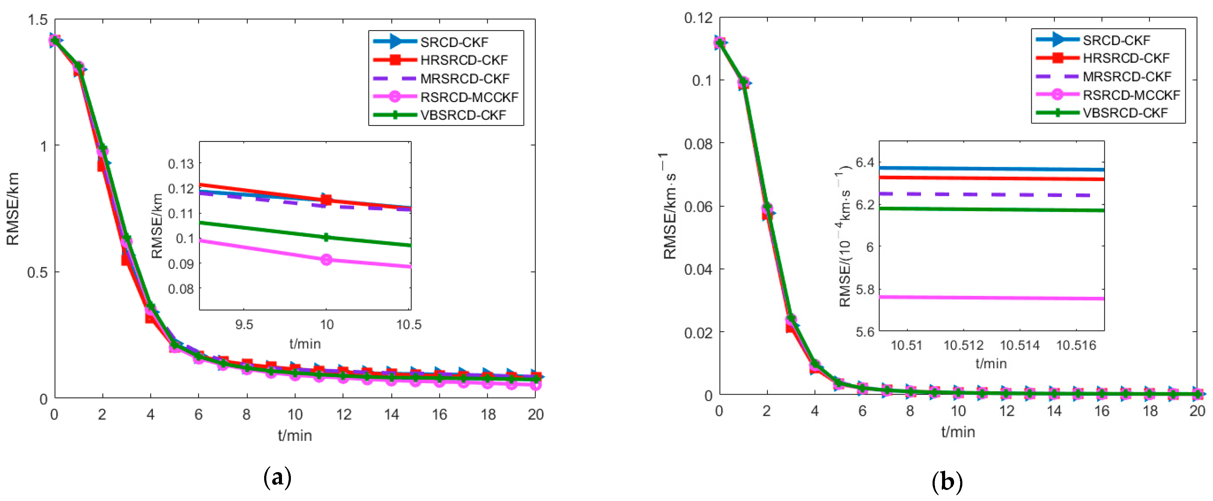
To evaluate the performance of the proposed methods, the remote distance passive target tracking scenario [27] is considered. The motion model of the target is the coordinated turn, analyzing the performance changes of the four continuous–discrete robust algorithms proposed in this paper for data with Gaussian noise (Section 4.1), non-Gaussian noise (Section 4.2), or corrupted by outliers (Section 4.3). When considering random interference, coordinated turn motion is a typical nonlinear motion. The continuous-time motion model can be expressed by stochastic differential equation.

The state vector of the target is $x\left(t\right)={\left[\begin{array}{ccccc}x\left(t\right)& \dot{x}\left(t\right)& y\left(t\right)& \dot{y}\left(t\right)& \mathsf{\omega }\end{array}\right]}^{\mathrm{T}}$; $x\left(t\right)$ and $y\left(t\right)$, $\dot{x}\left(t\right)$ and $\dot{y}\left(t\right)$ are the position and velocity of the target in the Cartesian coordinate system, respectively; and $\mathsf{\omega }$ is a constant turn rate, which is 0.01 rad/s. The motion of single observer in the CA model with the initial state is ${\left[0\mathrm{km},-0.025\mathrm{km}/\mathrm{s}, 0\mathrm{km}, 0.02\mathrm{km}/\mathrm{s}\right]}^{\mathrm{T}}$. The state equation of the system is $F\left(x\left(t\right)\right)={[\dot{x}\left(t\right),-\mathsf{\omega }\dot{y}\left(t\right),\dot{y}\left(t\right),\mathsf{\omega }\dot{x}\left(t\right),0]}^{\mathrm{T}}$. The random noise term is $w\left(t\right)={[w_1\left(t\right),w_2\left(t\right),w_3\left(t\right),w_4\left(t\right),w_5\left(t\right)]}^{\mathrm{T}}$, where its increment and state are independent of each other. Initial covariance matrix $Q=\mathrm{diag}[\begin{array}{ccccc}0& {\mathsf{\tau }}_1^{}& 0& {\mathsf{\tau }}_1^{}& {\mathsf{\tau }}_2^{}\end{array}]$, where ${\mathsf{\tau }}_1=\sqrt{2}$ and ${\mathsf{\tau }}_2=7\times {10}^{-6}$. The initial state $x\left(t_0\right)={[40\mathrm{km}, 0\mathrm{km}/\mathrm{s}, 50\mathrm{km}, 0.2\mathrm{km}/\mathrm{s}, 0.01\mathrm{rad}/\mathrm{s}]}^{\mathrm{T}}$, and the initial covariance matrix $P\left(t_0\right)=\mathrm{diag}[\begin{array}{ccccc}0.01& 0.01& 0.01& 0.01& 0\end{array}]$. The measurement sampling interval is 1 min. The number of Monte Carlo simulations is 200. The experiment is based on the MATLAB simulation software with an Intel(R) Core (TM) i7-10750H CPU @ 2.60 GHz 2.59 GHz.

Among them, the critical value of abnormal error discrimination in the HRSRCD-CKF algorithm is c = 1.345, the $\mathsf{\alpha }$ quantile of the chi-square distribution in the MRSRCD-CKF algorithm is ${\mathsf{\alpha }}_1=0.1,{\mathsf{\alpha }}_2=0.1\%$, the Gaussian kernel bandwidth $\mathsf{\sigma }$ in the RSRCD-MCCKF algorithm is selected according to the simulation scenarios, the initial parameters in the VBSRCD-CKF algorithm are $v_0=600$, $V_0=0.01$, $\mathsf{\rho }=1-\exp \left(-4\right)$, and the number of internal loops of the algorithm is M = 10.

The discrete-time nonlinear measurement model is

$$z_k=\left[{\tan }^{-1}\left(y_r\left(t_k\right)/x_r\left(t_k\right)\right)\right]+r_k,$$

(38)

where $x_r\left(t_k\right)$ and $y_r\left(t_k\right)$ are the relative position of the target and the observer at time k, $r_k$ is the measurement noise, and the specific expression form is defined according to the simulation scenarios.

In order to evaluate the performance of filtering, the Root Mean Square Error (RMSE) of the position state and the velocity state are respectively defined as

$$\mathrm{R}\mathrm{M}\mathrm{S}{\mathrm{E}}_{\mathrm{p}\mathrm{o}\mathrm{s}}\left(t_k\right)={\left(\frac{1}{N}{\displaystyle \sum _{i=1}^N{‖x\left(t_k\right)-{\hat{x}}_{}^i\left(t_k\right)‖}_2^2}\right)}^{1/2},$$

(39)

$$\mathrm{R}\mathrm{M}\mathrm{S}{\mathrm{E}}_{\mathrm{v}\mathrm{e}\mathrm{l}}\left(t_k\right)={\left(\frac{1}{N}{\displaystyle \sum _{i=1}^N{‖\dot{x}\left(t_k\right)-{\hat{\dot{x}}}_{}^i\left(t_k\right)‖}_2^2}\right)}^{1/2},$$

(40)

where N is the number of Monte Carlo simulations, ${\hat{x}}_{}^i\left(t_k\right)$ and ${\hat{\dot{x}}}_{}^i\left(t_k\right)$ are the results of the i-th Monte Carlo state estimation, and $x\left(t_k\right)$, $\dot{x}\left(t_k\right)$ are the true position state and velocity state of the target, respectively. The trajectory of target and observer is shown in Figure 1.

Figure 1. The trajectory of target and observer.

As shown in Figure 1, the bearings-only tracking scenario is tracking a two-dimensional target that is moving in a coordinated turn at a constant turn rate. The observer is maneuvered to achieve observability. In addition, it should be noted that the target tracked in this paper is the interference source on the ground, and the purpose of this paper is to improve the accuracy and robustness of this tracking process in different measurement environments through the continuous–discrete robust method.

4.1. Gaussian Noise

The measurement noise $r_k$ satisfies the Gaussian distribution with zero mean, that is, $r_k~N(\mathbf{0},R_k)$. The initial value of $R_k$ is a one-dimensional constant value of 0.001 rad. Before comparing the proposed algorithms, the influence of Gaussian kernel bandwidth $\mathsf{\sigma }$ on the algorithm RSRCD-MCCKF is discussed. The $\mathrm{R}\mathrm{M}\mathrm{S}{\mathrm{E}}_{\mathrm{p}\mathrm{o}\mathrm{s}}$ and $\mathrm{R}\mathrm{M}\mathrm{S}{\mathrm{E}}_{\mathrm{v}\mathrm{e}\mathrm{l}}$ of the algorithm at the final time instant are shown in Table 1.

Table 1. Algorithm accuracy under Gaussian noise when kernel bandwidth is different.

Algorithms	$\mathrm{R}\mathrm{M}\mathrm{S}{\mathrm{E}}_{\mathrm{p}\mathrm{o}\mathrm{s}}$$\left[\mathrm{km}\right]$	$\mathrm{R}\mathrm{M}\mathrm{S}{\mathrm{E}}_{\mathrm{v}\mathrm{e}\mathrm{l}}$$[\mathrm{km}\cdot {\mathrm{s}}^{-1}]$
RSRCD-MCCKF ($\mathsf{\sigma }=0.1$)	—	—
RSRCD-MCCKF ($\mathsf{\sigma }=1$)	0.0528	0.000205
RSRCD-MCCKF ($\mathsf{\sigma }=2$)	0.0449	0.000188
RSRCD-MCCKF ($\mathsf{\sigma }=5$)	0.0482	0.000179
RSRCD-MCCKF ($\mathsf{\sigma }=10$)	0.0645	0.000211
RSRCD-MCCKF ($\mathsf{\sigma }=50$)	0.0771	0.000239
SRCD-CKF	0.0784	0.000247

As shown in Table 1, when the Gaussian kernel bandwidth $\mathsf{\sigma }$ changes, the algorithm shows different performance. When the value of $\mathsf{\sigma }$ is too small or too large, the filtering accuracy will be reduced. Among them, — refers to the filtering as diverged. When the value of $\mathsf{\sigma }$ increases gradually, its filtering performance has approached the SRCD-CKF algorithm, which is in line with the previous theoretical derivation. But under the premise of $\mathsf{\sigma }=50$, its filtering accuracy is still higher than the SRCD-CKF algorithm. In other words, as long as the proper value of $\mathsf{\sigma }$ is selected, the filtering accuracy of the RSRCD-MCCKF algorithm is higher than the traditional algorithm.

On this basis, the Gaussian kernel bandwidth $\mathsf{\sigma }=5$ is selected, and we can see the $\mathrm{R}\mathrm{M}\mathrm{S}{\mathrm{E}}_{\mathrm{p}\mathrm{o}\mathrm{s}}$ and $\mathrm{R}\mathrm{M}\mathrm{S}{\mathrm{E}}_{\mathrm{v}\mathrm{e}\mathrm{l}}$ comparison of each algorithm in Figure 2.

Figure 2. The RMSE comparison of each algorithm under Gaussian noise. (a) $\mathrm{R}\mathrm{M}\mathrm{S}{\mathrm{E}}_{\mathrm{p}\mathrm{o}\mathrm{s}}$ of each algorithm under Gaussian noise; (b) $\mathrm{R}\mathrm{M}\mathrm{S}{\mathrm{E}}_{\mathrm{v}\mathrm{e}\mathrm{l}}$ of each algorithm under Gaussian noise.

As shown in Figure 2, when the measurement noise is Gaussian noise, the previous trends of each algorithm are roughly the same, and they all tend to converge as the time increases. Among them, HRSRCD-CKF and MRSRCD-CKF have small fluctuations compared with the SRCD-CKF algorithm, and the accuracy is basically the same under normal measurement conditions. The accuracy of the VBSRCD-CKF algorithm is slightly higher than that of HRSRCD-CKF and MRSRCD-CKF; this reflects the higher accuracy of the variational Bayesian method in approximate estimation. The RSRCD-MCCKF has higher accuracy than the above algorithms, because the maximum correntropy criterion can utilize higher-order information of measurements, applying the Gaussian kernel to each element of the estimation error matrix, which has a better combination with SRCD-CKF.

4.2. Gaussian Mixture Noise

The measurement noise is Gaussian mixed noise. Gaussian mixed noise is a typical non-Gaussian distribution,$r_k~0.99N(\mathbf{0},R_k)+0.01N(\mathbf{0},\mathbf{500}\ast R_k)$. The $\mathrm{R}\mathrm{M}\mathrm{S}{\mathrm{E}}_{\mathrm{p}\mathrm{o}\mathrm{s}}$ and $\mathrm{R}\mathrm{M}\mathrm{S}{\mathrm{E}}_{\mathrm{v}\mathrm{e}\mathrm{l}}$ of the RSRCD-MCCKF algorithm at the final time instant, when the kernel bandwidth $\mathsf{\sigma }$ changes in the non-Gaussian noise environment, are shown in Table 2.

Table 2. Algorithm accuracy under non-Gaussian noise when kernel bandwidth is different.

Algorithms	$\mathrm{R}\mathrm{M}\mathrm{S}{\mathrm{E}}_{\mathrm{p}\mathrm{o}\mathrm{s}}$$\left[\mathrm{km}\right]$	$\mathrm{R}\mathrm{M}\mathrm{S}{\mathrm{E}}_{\mathrm{v}\mathrm{e}\mathrm{l}}$$[\mathrm{km}\cdot {\mathrm{s}}^{-1}]$
RSRCD-MCCKF ($\mathsf{\sigma }=2$)	—	0.0349
RSRCD-MCCKF ($\mathsf{\sigma }=3$)	1.0829	0.0043
RSRCD-MCCKF ($\mathsf{\sigma }=5$)	0.4716	0.0014
RSRCD-MCCKF ($\mathsf{\sigma }=7$)	0.4813	0.0014
RSRCD-MCCKF ($\mathsf{\sigma }=10$)	0.5375	0.0016
SRCD-CKF	0.6679	0.0019

As shown in Table 2, the value of $\mathsf{\sigma }$ that can suppress the non-Gaussian noise has changed. Compared with the Gaussian conditions, the filtering accuracy of the algorithms is reduced, but the appropriate $\mathsf{\sigma }$ can still suppress the non-Gaussian noise that appears in the measurement. Therefore, it is more important to adaptively select the value of $\mathsf{\sigma }$ according to different scenarios.

Here, the Gaussian kernel bandwidth $\mathsf{\sigma }=5$ is also selected under the condition of non-Gaussian noise. The $\mathrm{R}\mathrm{M}\mathrm{S}{\mathrm{E}}_{\mathrm{p}\mathrm{o}\mathrm{s}}$ and $\mathrm{R}\mathrm{M}\mathrm{S}{\mathrm{E}}_{\mathrm{v}\mathrm{e}\mathrm{l}}$ comparison of each algorithm is shown in Figure 3.

Figure 3. The RMSE comparison of each algorithm under non-Gaussian noise. (a) $\mathrm{R}\mathrm{M}\mathrm{S}{\mathrm{E}}_{\mathrm{p}\mathrm{o}\mathrm{s}}$ of each algorithm under non-Gaussian noise; (b) $\mathrm{R}\mathrm{M}\mathrm{S}{\mathrm{E}}_{\mathrm{v}\mathrm{e}\mathrm{l}}$ of each algorithm under non-Gaussian noise.

It can be seen from Figure 3 that when the measurement noise is non-Gaussian noise, the errors of each algorithm increase slightly. The HRSRCD-CKF algorithm and the MRSRCD-CKF algorithm cannot effectively suppress the non-Gaussian measurement noise, and the algorithm basically fails. The VBSRCD-CKF algorithm and the RSRCD-MCCKF algorithm can suppress non-Gaussian noise to a certain extent. The filtering performance of the two algorithms is basically equivalent and finally shows relatively high convergence accuracy, which reflects their ability to deal with non-Gaussian noise problems.

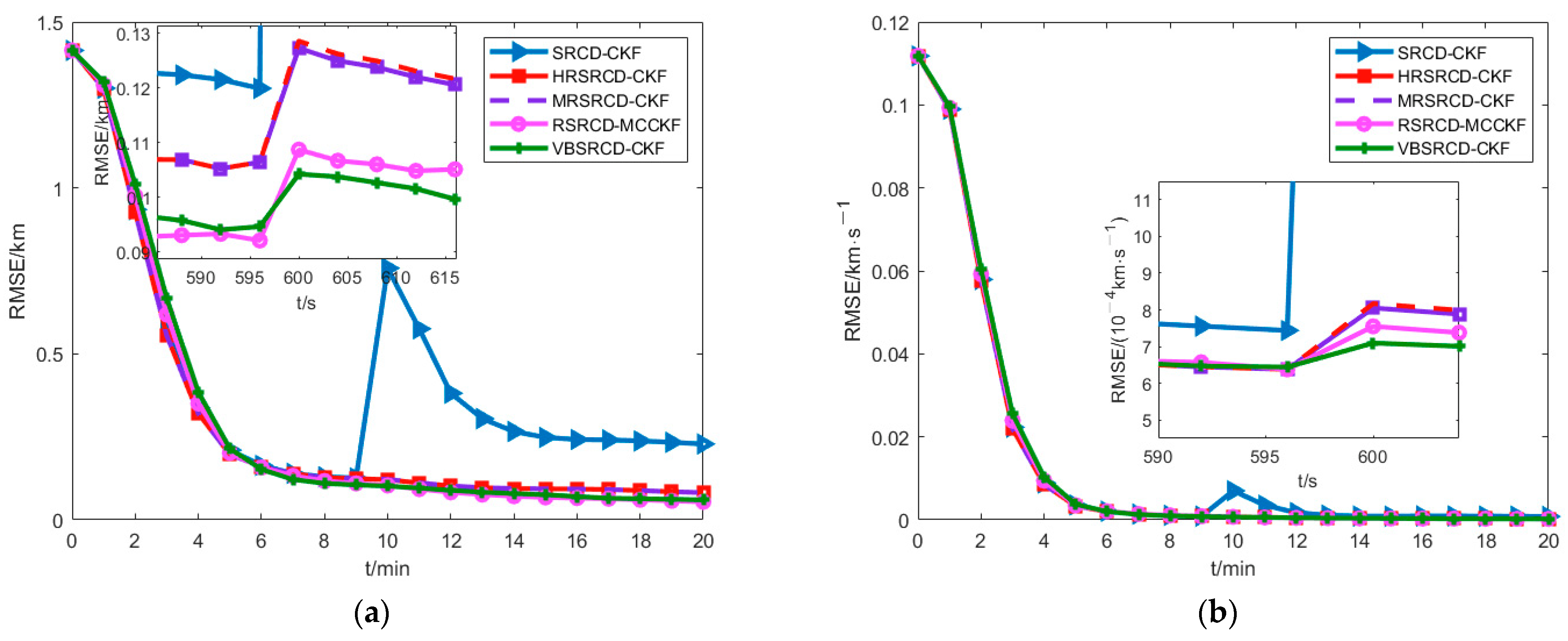
4.3. Gaussian Noise Together with Shot Noise

The measurement noise satisfies the Gaussian distribution with zero mean, and the measurement covariance matrix changes suddenly to 30 times the original at t = 10 min,$R_k^{10}=30R_k$. Considering that when $\mathsf{\sigma }=5$, the filtering performance in RSRCD-MCCKF is good regardless of Gaussian noise or non-Gaussian noise; consequently, we still choose $\mathsf{\sigma }=5$ here. The $\mathrm{R}\mathrm{M}\mathrm{S}{\mathrm{E}}_{\mathrm{p}\mathrm{o}\mathrm{s}}$ and $\mathrm{R}\mathrm{M}\mathrm{S}{\mathrm{E}}_{\mathrm{v}\mathrm{e}\mathrm{l}}$ of each algorithm are shown in Figure 4.

Figure 4. The RMSE comparison of each algorithm under abnormal measurement. (a) $\mathrm{R}\mathrm{M}\mathrm{S}{\mathrm{E}}_{\mathrm{p}\mathrm{o}\mathrm{s}}$ of each algorithm under abnormal measurement; (b) $\mathrm{R}\mathrm{M}\mathrm{S}{\mathrm{E}}_{\mathrm{v}\mathrm{e}\mathrm{l}}$ of each algorithm under abnormal measurement.

As shown in Figure 4, when the measurement is abnormal, the error of the SRCD-CKF algorithm increases abruptly, which is not robust. While the other algorithms effectively resist the abnormal measurement. Among them, the VBSRCD-CKF algorithm shows better robustness, and it has the most obvious effect on abnormal measurement suppression; the RSRCD-MCCKF algorithm is second only to the VBSRCD-CKF algorithm and shows good robustness with high accuracy, while the suppression effect of the HRSRCD-CKF algorithm and the MRSRCD-CKF algorithm is slightly worse, indicating that the RSRCD-MCCKF algorithm and the VBSRCD-MCCKF algorithm are more effective in dealing with abnormal measurement problems.

4.4. Computational Complexity

When comparing the computational complexity of each algorithm, the parameter settings are the same as in Section 4.1 and Section 4.3, respectively. The relative computation time of SRCD-CKF is set to “1”. The relative computation time of each algorithm is shown in Table 3.

Table 3. The relative computation time of each algorithm.

Algorithms	Computation Time (Scenario 4.1)	Computation Time (Scenario 4.3)
SRCD-CKF	1	1
HRSRCD-CKF	1.029	1.034
MRSRCD-CKF	1.005	1.018
RSRCD-MCCKF	1.076	1.080
VBSRCD-CKF	1.068	1.071

As shown in Table 3, the four robust algorithms all take longer than the initial SRCD-CKF algorithm, but their difference is not obvious. In addition, it can be observed that the computation time of each algorithm increases when interference is encountered, but the computation time has not increased much. Among them, the HRSRCD-CKF algorithm and the MRSRCD-CKF algorithm are relatively low in complexity. The computation time of the VBSRCD-CKF algorithm increases due to a certain number of inner loops. The computation time of the RSRCD-MCCKF is the longest because the calculation process includes more matrix inversion operations and exponential operations of Gaussian kernel function. However, considering the accuracy of the algorithm and application scenarios, it is acceptable within a similar time period.

Furthermore, it can be seen that the computation time of the proposed algorithms are longer than initial algorithm, but its improvement in accuracy and robustness is critical, which is the focus of this research. At the same time, considering that the increase in computing time is not obvious, the proposed algorithms can be used for other filtering problems.

5. Conclusions

In this paper, in order to evaluate the performance of robust methods in continuous–discrete tracking systems, four robust square-root continuous–discrete cubature Kalman filter algorithms are proposed. From the results, we can draw the following conclusions:

(1)

The effectiveness of the algorithms in this paper is evaluated through a remote distance passive target tracking scenario, and the simulation results demonstrate the better environmental adaptability of the proposed algorithms in solving continuous-discrete robust problems. What’s more, this paper aims to solve the slow tracking problem in remote distance passive target tracking, and the proposed algorithms can also be used in other navigation domains.

(2)

As a common tool for data processing, Huber’s estimation has a wide range of applications. The RSRCD-MCCKF algorithm and the VBSRCD-CKF algorithm proposed in this paper are better than the Huber’s estimator, which provides an alternative means for the field of robust estimation.

(3)

In the simulation results, we can see that the filtering performance of the algorithm without robustness is very poor. Therefore, when the system’s data are contaminated by outliers, the relevant robust estimation method is indispensable.

References

- He, R.K.; Chen, S.X.; Wu, H.; Chen, K.; Liu, J. Adaptive Covariance Feedback Cubature Kalman Filtering for Continuous-Discrete Bearings-Only Tracking System. IEEE Access 2019, 7, 2686–2694. [Google Scholar] [CrossRef]
- Li, L.Q.; Wang, X.L.; Liu, Z.X.; Xie, W.X. Auxiliary truncated unscented Kalman filter for bearings-only maneuvering target tracking. Sensors 2017, 17, 972. [Google Scholar] [CrossRef] [PubMed]
- Crouse, D. Basic tracking using nonlinear continuous-time dynamic models. IEEE Aerosp. Electron. Syst. Mag. 2015, 30, 4–41. [Google Scholar] [CrossRef]
- Arasaratnam, I.; Haykin, S.; Hurd, T.R. Cubature Kalman Filtering for Continuous-Discrete Systems: Theory and Simulation. IEEE Trans. Signal Processing 2010, 58, 4977–4993. [Google Scholar] [CrossRef]
- Crouse, D.F. Cubature Kalman Filters for Continuous-Time Dynamic Models Part I: Solutions Discretizing the Langevin Equation. In Proceedings of the 2014 IEEE Radar Conference, Cincinnati, OH, USA, 19–23 May 2014. [Google Scholar]
- Crouse, D.F. Cubature Kalman Filters for Continuous-Time Dynamic Models Part Ⅱ: A Solution Based on Moment Matching. In Proceedings of the 2014 IEEE Radar Conference, Cincinnati, OH, USA, 19–23 May 2014. [Google Scholar]
- Kulikov, G.Y.; Kulikova, M.V. Accurate Numerical Implementation of the Continuous-Discrete Extended Kalman Filter. IEEE Trans. Autom. Control 2014, 59, 273–279. [Google Scholar] [CrossRef]
- Wang, J.L.; Zhang, D.X.; Shao, X.W. New version of continuous-discrete cubature Kalman filtering for nonlinear continuous-discrete systems. ISA Trans. 2019, 91, 174–783. [Google Scholar] [CrossRef]
- Kulikov, G.Y.; Kulikova, M.V. NIRK-based Accurate Continuous-Discrete Extended Kalman filters for Estimating Continous-Time Stochastic Target Tracking Models. J. Comput. Appl. Math. 2016, 316, 260–270. [Google Scholar] [CrossRef]
- He, R.K.; Chen, S.X.; Wu, H.; Chen, K. Stochastic feedback based continuous-discrete cubature Kalman filtering for bearings-only tracking. Sensors 2018, 18, 1959. [Google Scholar] [CrossRef]
- Gordon, N.J.; Salmond, D.J.; Smith, A.F.M. Novel Approach to Nonlinear/Non-Gaussian Bayesian State Estimation. Radar Signal Processing IEE Proc. Part F 1993, 140, 107–113. [Google Scholar] [CrossRef]
- Arulampalam, M.S.; Maskell, S.; Gordon, N.; Clapp, T. A tutorial on particle filters for online nonlinear/non-Gaussian Bayesian tracking. IEEE Trans. Signal Processing 2002, 50, 174–188. [Google Scholar] [CrossRef]
- Meinhold, R.J.; Singpurwalla, N.D. Robustification of Kalman filter methods. J. Am. Stat. Assoc. 1989, 84, 479–486. [Google Scholar] [CrossRef]
- Huber, P.J.; Ronchetti, E.M. Robust Statistics, 2nd ed.; Wiley: Hoboken, NJ, USA, 2009. [Google Scholar]
- Jureckova, J.; Picek, J.; Schindler, M. Robust Statistical Methods with R, 2nd ed.; CRC Press: Boca Raton, FL, USA, 2019. [Google Scholar]
- Chang, J.B.; Liu, M. M-estimator-based robust Kalman filter for systems with process modeling errors and rank deficient measurement models. Nonlinear Dyn. 2015, 80, 1431–1449. [Google Scholar] [CrossRef]
- Wu, H.; Chen, S.X.; Chen, K.; Yang, B.F. Robust cubature Kalman filter target tracking algorithm based on genernalized M-estiamtion. Acta Phys. Sin. 2015, 64, 456–463. [Google Scholar] [CrossRef]
- Wu, H.; Chen, S.X.; Chen, K.; Yang, B.F. Robust Derivative-Free Cubature Kalman Filter for Bearings-Only Tracking. J. Guid. Control. Dyn. 2016, 39, 1865–1870. [Google Scholar] [CrossRef]
- Särkkä, S.; Nummenmaa, A. Recursive noise adaptive Kalman filtering by variational Bayesian approximations. IEEE Trans. Autom. Control. 2009, 54, 596–600. [Google Scholar] [CrossRef]
- Wang, G.Q.; Li, N.; Zhang, Y.G. Maximum correntropy unscented Kalman and information filters for non-Gaussian measurement noise. J. Frankl. Inst. 2017, 354, 8659–8677. [Google Scholar] [CrossRef]
- Liu, X.; Qu, H.; Zhao, J.; Yue, P.; Wang, M. Maximum correntropy unscented Kalman filter for spacecraft relative state estimation. Sensors 2016, 16, 1530. [Google Scholar] [CrossRef]
- Liu, X.; Chen, B.; Xu, B.; Wu, Z.; Honeine, P. Maximum correntropy unscented filter. Int. J. Syst. Sci. 2017, 48, 1607–1615. [Google Scholar] [CrossRef]
- Särkkä, S.; Solin, A. On continuous-discrete cubature Kalman filtering. IFAC Proc. Vol. 2012, 45, 1221–1226. [Google Scholar] [CrossRef]
- Särkkä, S. On unsented Kalman filtering for state estimation of continuous-time nonlinear systems. IEEE Trans. Autom. Control 2007, 52, 1631–1641. [Google Scholar] [CrossRef]
- Chen, B.D.; Liu, X.; Zhao, H.Q.; Principe, J.C. Maximum correntropy Kalman filter. Automatica 2017, 76, 70–77. [Google Scholar] [CrossRef]
- Särkkä, S.; Hartikainen, J. Non-linear noise adaptive Kalman filtering via variational Bayes. In Proceedings of the IEEE International Workshop on Machine Learning for Signal Processing (MLSP) Conference, Southampton, UK, 22–25 September 2013. [Google Scholar]
- He, R.K.; Chen, S.X.; Wu, H.; Zhang, F.Z.; Chen, K. Efficient extended cubature Kalman filtering for nonlinear target tracking. Int. J. Syst. Sci. 2020, 52, 392–406. [Google Scholar] [CrossRef]
Publisher’s Note: MDPI stays neutral with regard to jurisdictional claims in published maps and institutional affiliations. |
© 2022 by the authors. Licensee MDPI, Basel, Switzerland. This article is an open access article distributed under the terms and conditions of the Creative Commons Attribution (CC BY) license (https://creativecommons.org/licenses/by/4.0/).