Abstract
Automatic guided vehicles have become an important part of transporting goods in dynamic environments, and how to design an efficient path planning method for multiple AGVs is a current research hotspot. Due to the complex road conditions in dynamic environments, there may be dynamic obstacles and situations in which only the target point is known but a complete map is lacking, which leads to poor path planning and long planning time for multiple automatic guided vehicles (AGVs). In this paper, a two-level path planning method (referred to as GA-KL, genetic KL method) for multi-AGVs is proposed by integrating the scheduling policy into global path planning and combining the global path planning algorithm and local path planning algorithm. First, for local path planning, we propose an improved Q-learning path optimization algorithm (K-L, Kohonen Q-learning algorithm) based on a Kohonen network, which can avoid dynamic obstacles and complete autonomous path finding using the autonomous learning function of the Q-learning algorithm. Then, we adopt the idea of combining global and local planning by combining the K-L algorithm with the improved genetic algorithm; in addition, we integrate the scheduling policy into global path planning, which can continuously adjust the scheduling policy of multi-AGVs according to changes in the dynamic environment. Finally, through simulation and field experiments, we verified that the K-L algorithm can accomplish autonomous path finding; compared with the traditional path planning algorithm, the algorithm achieved improves results in path length and convergence time with various maps; the convergence time of the algorithm was reduced by about 6.3%, on average, and the path length was reduced by about 4.6%, on average. The experiments also show that the GA-KL method has satisfactory global search capability and can effectively avoid dynamic obstacles. The final experiments also demonstrated that the GA-KL method reduced the total path completion time by an average of 12.6% and the total path length by an average of 8.4% in narrow working environments or highly congested situations, which considerably improved the efficiency of the multi-AGVs.
1. Introduction
1.1. Motivation and Incitement
As human needs change, the environment in which AGVs work has changed from a static, indoor, unmanned factory to a dynamic special environment, such as a mine or a forest [1]. This special dynamic working environment has three distinct characteristics: 1. the presence of dynamic obstacles; 2. a lack of a complete map; and 3. a small working space. Therefore, path planning of multi-AGVs is associated with three important problems waiting to be solved: 1. how to efficiently avoid unknown dynamic obstacles; 2. how to efficiently complete path planning in the absence of accurate maps, with only a small amount of coordinate information of target points; and 3. how to coordinate path planning of multiple AGVs to ensure transportation efficiency even in a narrow environment [2]. Given the above problems, dynamic path planning of AGVs based on special environments has become a research hotspot [3]. It is important to establish a method that can accomplish dynamic path planning of multiple AGVs in order to maximize the transportation time of AGVs in dynamic environments.
1.2. Literature Review and Contribution
Path planning is further divided into local and global planning, depending on the environment [4]. Global path optimization algorithms are suitable for static environments, as they require complete map information [5]. Local path planning algorithms collect information about the environment through sensors and dynamically generate planning tasks [6]. The main objective of AGV path planning is to select the least costly and collision-free path from the starting point to the end point. Traditional path planning methods for multi-AGVs include the artificial potential field method [7], fuzzy logic algorithm [8], genetic algorithms [9], particle swarm optimization algorithms [10], etc. Traditional path planning algorithms have good search capability, but they require accurate maps or high-precision sensors in dynamic environments, resulting in unsatisfactory actual planning results.
Based on the above problems, in the field of local path planning, many scholars have applied Q-learning algorithms as the research direction because the autonomous learning capability of Q-learning algorithms can be used to accomplish pathfinding and avoid dynamic obstacles in unknown environments in the absence of accurate maps and high-precision sensors [11]. Q-learning algorithms are used to obtain the reward value of the environmental feedback through the continuous interaction between the agent and the environment, and then obtain the ideal policy by maximizing the long-term compensation. Traditional Q-learning algorithms are applicable to simple environments; however, AGVs work in a complex 3D space. For Q-learning algorithms, complex environments lead to more complex actions, resulting in huge Q-tables (a Q-table is a mapping table of actions to reward values). Because AGVs traverse the Q-table for each step forward, this leads to slow convergence and poor planning results, which is unacceptable for practical planning tasks. Scholars have made a series of improvements to alleviate this problem. Yung NC [12] proposed an adaptive heuristic critic (AHC) algorithm, which classifies and generalizes the input information through neurons so that the continuous state can be discretized. However, AHC converges slowly and faces the problem of “the curse of dimensionality”. Hengst [13] used a hierarchical reinforcement learning algorithm to reduce the number of states, but this method requires considerable prior knowledge in order to build a hierarchical structure. Xie [14] proposed heuristic Q-learning based on experience replay for three-dimensional path planning (HQ), which reduces the number of useless explorations by constructing heuristic functions with RL. In summary, although many scholars have used traditional neural networks or an a priori knowledge base to optimize Q-learning algorithms so that the number of states is reduced, in the absence of training samples, a classification effect cannot be achieved; therefore, the problem of a large state space cannot be solved by Q-learning algorithms, and the algorithm optimization effect is poor. Moreover, the “explore-and-use” strategy is static, and the algorithm does not receive timely feedback when there are dynamic obstacles, resulting in low learning efficiency.
In a dynamic environment, Q-learning algorithms obtain the same environmental information, such as static cargo containers, charging piles, walls, etc., with high probability, and different environmental information only when dynamic obstacles are present. Therefore, clustering algorithms should be used to classify dynamic environmental information and reduce the size of the Q-table as much as possible to speed up the convergence of the algorithm. However, in a dynamic environment, a large amount of dynamically changing information is collected by sensors, and there are no relevant training samples to help clustering algorithms complete their training; therefore, it is difficult to complete the clustering work with traditional clustering algorithms, such as hierarchy-based clustering algorithms, k-means, etc. [15]. In this paper, we take advantage of the properties of a Kohonen network of automatic environment recognition and automatic classification of environmental information (a Kohonen network is a self-organizing mapping network that works via unsupervised learning) to optimize the Q-learning algorithm [16]. Automatically identifying and classifying environmental information can shrink Q-tables and turn complex 3D spaces into streamlined mapping networks [17].
However, in a dynamic environment, a local path planning algorithm avoids dynamic obstacles by sacrificing time and only performs local instead of global searches, which leads to an unsatisfactory effect of multi-AGV path planning. Therefore, many scholars have combined global path planning algorithms and local path planning algorithms to obtain improved planning results [18]. Yong-Kyun [19] adopted a three-layer control architecture model and proposed an obstacle avoidance algorithm integrating a global planning algorithm and the artificial potential method to effectively accomplish obstacle avoidance tasks in a dynamic environment. The artificial potential field method used in this method is a feedback control strategy that is robust to control sensing errors; however, it suffers from a local minimum problem and is therefore not guaranteed to find a locally optimal path. H.W. Griepentrog [20] built a six-layer structured network containing three main components: path planning, information collection, and autonomous navigation. Griepentrog’s network involves two layers of path planning: static planning and dynamic planning. Dynamic planning can be subdivided into costing and path optimization; two layers of information collection: intelligent detection and environmental information collection and fusion; two layers of autonomous navigation: localization and guidance, and path selection. This method requires high-precision sensors to collect environmental information, and the sensor accuracy of common AGVs is not high. In addition, this method uses a BP neural network to classify environmental information, which leads to unsatisfactory classification results.
The above methods only combine global and local algorithms but lack consideration of the actual environment, such as road conditions, sensor accuracy of AGVs, etc. More critically, they lack scheduling between AGVs and analysis of the current congestion, so they are not suitable for the actual working environment. We use road conditions and congestion as constraints to improve the genetic algorithm (T-GA) and will evaluate the congestion of the working environment for the scheduling of multiple AGVs. Finally, we combine the improved genetic algorithm with the K-L algorithm to propose a path planning method for multiple AGVs that is suitable for real dynamic working environments.
To further improve the efficiency of AGVs, many scholars have combined scheduling and path planning. For example, Yang designed a Flexsim simulation model of AGVs in a manufacturing plant, which can be used to study the shortest motion path and lowest cost of AGVs [21]. Zhang considered a method to improve the operational efficiency of the system, which combines a task assignment strategy based on a genetic algorithm (GA) and a path planning strategy based on reinforcement learning (RL) [22].
The above methods all obtain task assignment schemes through scheduling first and then perform path planning, rarely performing both tasks simultaneously. Therefore, if the work environment changes, the new task assignment scheme cannot be instantly fed back to the path planning. Therefore, we integrate the scheduling policy into the T-GA-based global path planning process, which can continuously adjust the scheduling policy according to the changes in time and environment.
In summary, in this paper, we propose a two-layer path planning method for multiple AGVs that can efficiently solve the three problems faced by AGVs. The main contributions of this paper are as follows:
- (1)
- To solve the problem of dynamic obstacle avoidance and unknown environment pathfinding for AGVs, we design an improved Q-learning path optimization algorithm based on Kohonen networks (K-L for short).
- (2)
- In order to obtain improved path planning results, we propose a two-level path planning method by combining a K-L algorithm and an improved genetic algorithm (referred to as GA-KL). We use a genetic algorithm (T-GA) based on path smoothing factor and node busy factor optimization as a global planning algorithm to generate the global optimal set of path nodes.
- (3)
- To effectively accomplish dynamic scheduling of multi-AGVs, we integrate the scheduling policy into global path planning and achieve dynamic scheduling of multiple AGVs by analyzing the congestion of the current working environment and combining it with a weight-based voting algorithm.
1.3. Paper Organization
The rest of this paper is organized as follows. In Section 2, an action state-space model is designed, and a local path planning algorithm based on a K-L algorithm is proposed. In Section 3, the genetic algorithm is optimized, and a global path planning algorithm based on the improved genetic algorithm is proposed. In Section 4, we combine the K-L algorithm and the improved genetic algorithm to propose a two-level path planning method. In Section 5, we present the experimental results. In Section 6, we conclude the paper and discuss future work.
2. K-L-Based Local Path Planning Algorithm
2.1. Design of Action State-Space Model
AGVs receive environmental information with five sensors, each facing a different direction: −90°, −45°, 0°, 45°, and 90°. With the stipulation of the AGV not to moving backwards, no sensor is located at the rear. The environmental information collected by the sensors, including the straight-line distance between the AGV and the obstacle, is later used as the state of reinforcement learning.
Under general circumstances, three executable actions are available for the AGV: driving straight ahead, driving 45° to the left, or driving 45° to the right. The positions of the sensors and the performable actions of the AGV are shown in Figure 1.
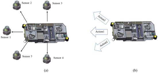
Figure 1.
Sensor placement and movement direction. (a) shows the position where the sensor is placed, and (b) shows the forward direction of AGVs.
2.2. Adaptive Clustering Method Based on Kohonen Network
2.2.1. Implementation of Adaptive Clustering Method Based on Kohonen Network
In accordance with the number of sensors shown in Figure 1, five neurons are set up in the network input, receiving the measured distances of each sensor as data . The input layer has an extra neuron, which is defined as constant and represents the largest reward of the AGV in the current action. Each neural unit of the output layer consists of a triplet , where is the corresponding state, is the score of each action in the current state, and these two values are used to select the action ().
The computation process is as follows:
- (1)
- The input sample represents the distance between the AGV and the obstacle. The input initialization vector is , and the weights of the connections between all input and output nodes are , . The number of neurons in the input layer is , and the output layer is .
- (2)
- Construct the Kohonen network.
- (3)
- Initialize the learning rate (), the neighborhood (), and the maximum number of iterations ().
- (4)
- Feed input feature vector .
- (5)
- Calculate the similarity between and by Euclidean distance. Eventually, the output node (j*) with the minimum distance is selected.
The neuron with the shortest is the winning neuron. In the formula, the weights of the connections between all input and output nodes are ; the number of neurons in the input layer is , and the output layer is . The input initialization vector is .
- (6)
- Adjust the connection weights of the winning neuron and its neighborhood, .
- (7)
- Check if the network converges. Implement (1) if it converges; otherwise, exit.
According to the above design, the number of states generated by the Q-learning algorithm in the learning process is .
2.2.2. Analysis of Discrete State
The states in a dynamic environment are discrete states. Setting up discrete states is usually achieved by dividing them based on the maximum distance sensed by the sensors and the distance between the sensors and the obstacles. Excessively coarse segmentation can lead to suboptimal path planning for AGVs, whereas excessively fine segmentation can lead to “dimensional disaster” problems and slow down the convergence of the algorithm. For example, when the shape of the obstacle is regular, the sensor and the obstacle distance generally only need to be divided into four states, indicating that the obstacle is one-third distance or two-thirds distance from the sensor, as well as the maximum measurement distance of the sensor and the range beyond. However, when the shape of the obstacle is irregular, the division accuracy needs to be continuously improved to ensure the learning efficiency of the algorithm.
The following table shows the “state action” pairs of the Q-learning algorithm for AGVs with varying segmentation accuracies. In this case, the number of sensors of the AGV is five, and the number of allowed actions is three. As shown in the table below, the “state-action” pairs of the Q-learning algorithm increase dramatically with the number of divisions, making it difficult to determine which division is the most appropriate. Moreover, in the actual learning process, there are many similar states, but because each state is learned and an action is selected by looking up the table to traverse each state, this considerably affects the learning efficiency of the algorithm.
Given the above problems, we use automatic environment recognition and the automatic environment information classification function of a Kohonen network to classify the environmental information and reduce the size of Q-table as much as possible to speed up the convergence of the algorithm.
Assuming that the number of neurons in the output layer of the Kohonen network is 50 and the number of AGV sensors is 5, according to Section 2.2.1, we can calculate the total number of states as 300. Table 1 shows that the current total number of states is significantly reduced. In addition, with the help of the Kohonen network, there is no need to consider how to divide the accuracy more reasonably.

Table 1.
Number of distance divisions and number of states.
2.3. Exploration Strategy Based on a Self-Adapting Simulated Annealing Algorithm
Traditional Q-learning algorithms determine the exploration strategy according to a constant . The exploration strategy has a probability of choosing an arbitrary action and a probability of of choosing the best action in the current scenario. A fixed value of in the static environment does not affect the learning efficiency of the algorithm, but in the dynamic environment, especially when dynamic obstacles appear, if is too large, the Q-learning algorithm will hardly converge, whereas if is too small, the Q-learning algorithm will easily converge to the local optimal solution. Therefore, for a dynamic environment, an adaptive simulated annealing algorithm (SSA for short) is used in this paper to dynamically adjust the value of . The formula is as follows:
Variations of the Q-value are expressed as , and is the temperature of iteration , which continues to decrease.
We can infer from the formula that when the Q-value increases, the SSA-based strategy tends to explore a new action, and when the Q-value decreases, the strategy has a probability of of choosing the best action in the current scenario. As continues to decrease, the K-L algorithm has a high probability of exploring new actions during the early stage of training and a high probability of choosing to exploit existing experience in the later stages of training.
The decay of is a linear process, whereas the change in value is nonlinear. Therefore, we select the maximum of both and the fixed annealing rate () as the actual annealing rate of the SSA. The actual annealing rate can be adjusted according to the variation of values, so when the variation of values is too large, the SSA-based strategy obtains a large value, and there is a high possibility of exploring new actions; as a result, the K-L algorithm is prevented from obtaining a locally optimal solution.
where denotes the Q-value after iterations, is the decay factor, and is a normalization function. According to Equation (5), slowing down the temperature drop in the early stage when the Q-value changes drastically adds more explorability to the suboptimal path, whereas accelerating the temperature drop in the later stage near convergence and decreasing makes the algorithm less exploratory, resulting in stable convergence.
In summary, the SSA algorithm controls the initial temperature and the temperature decay function, and the Q-value matrix stabilizes with an increasing number of iterations so that ε decreases gradually with successive iterations of the algorithm. The Q-learning algorithm ensures sufficient exploration of the path in the early stage and stable convergence in the later stage.
2.4. Reward Function
For the reward function of traditional Q-learning algorithms, if the AGV reaches the end point, it yields a reward, whereas if it collides with obstacles, it yields a penalty. For other situations, the reward function of the AGV yields a “reward” value of 0. The traditional reward function has the advantages of simple calculation and ease of implementation. However, for the path optimization problems of the AGVs, if the number of states is large and the number of dimensions is larger, when the feedbacks of many states are 0, the learning efficiency of the Q-learning algorithm is reduced and the convergence time increases. Therefore, we utilize potential energy to improve the traditional reward function.
We simulate the working environment of the AGV as a potential energy field. The end point generates gravitational potential energy, whereas the obstacle generates repulsive potential energy. As a result, when the AGV approaches the end point, it obtains an extra reward value. Conversely, when the AGV moves away from the end point or collides with an obstacle, it loses the reward.
The improved reward function is as follows:
where is the reward obtained when the AGV reaches the target point, is the penalty value obtained when (the distance between the AGV and the obstacle) is equal to 0, and is a penalty value. is the potential energy of the current time (), and is the current additional reward value. is the distance between the AGV and obstacles. The calculation formulae of and are as follows:
where is the straight-line distance between the AGV and the end point, and is the punishment factor.
If the AGV keeps approaching the target point, i.e., , a positive payoff () is obtained; if the AGV keeps moving away from the target point, a negative payoff () is obtained; and if the AGV reaches the destination, a large value is obtained. If the distance between the AGV and the target point is kept constant due to the presence of dynamic obstacles, the dynamic obstacle is used as a repulsive field; then, the payoff value is the value of the change in the distance between the AGV and the dynamic obstacle, as well as the change in the distance to the target point. If the action reduces the distance to the target point, then a positive payoff is obtained; otherwise, a negative payoff is obtained. This design allows the AGV to quickly avoid dynamic obstacles, in addition to providing the AGV with timely feedback on each action taken, ensuring continuity of the payoff function and accelerating the convergence of the algorithm.
2.5. The Flow of the K-L Algorithm
The K-L algorithm flow is shown in Figure 2. The main steps of the optimal path algorithm based on K-L are as follows:
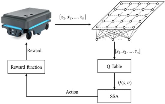
Figure 2.
Algorithm flow chart.
- (1)
- When the sensors find an obstacle, the K-L algorithm is activated:
- (2)
- First, the Kohonen network outputs the state set (), which records the information collected by the sensors.
- (3)
- Then, the algorithm establishes a state–action mapping pair. The mapping pair is established by traversing the actions of each state (for example, the AGV moves forward). The mapping pair is represented by and is stored in the Q-table.
- (4)
- Then, the SSA-based exploration strategy selects the next action based on the Q-table. Finally, the AGV obtains the reward value of environmental feedback.
- (5)
- The AGV selects the next action according to the reward value of environmental feedback until it bypasses the obstacle.
2.6. Time Complexity Analysis of the K-L
Suppose the complexity scale of the problem to be solved is . As shown in Table 2, the time complexity of the algorithm after iterations is .

Table 2.
Time complexity analysis.
2.7. Space Complexity Analysis of the K-L
The space complexity of the K-L algorithm is . Traditional Q-learning algorithms adopt the setting method of discrete state, which is generally divided according to the maximum distance () perceived by the sensor and the distance () between the sensor and the obstacle. The discrete states and corresponding operations are added to the Q-table. Because each state and action selection of the Q-learning algorithm traverse each state, checking the table, the Q-table determines the space complexity of the Q-learning algorithm. Assuming that the number of sensors is and the number of obstacles is , the space complexity of adaptive clustering through the Kohonen network is only (when the number of clusters is ).
3. Global Path Planning Algorithm Based on the Improved Genetic Algorithm
A distinctive feature in dynamic environments is the lack of complete map information; an AGV may only have the coordinates of a few target points. Compared with other global path planning algorithms, genetic algorithms require less map accuracy and can define a limited number of target points as chromosome variants to accomplish path planning between target points and incorporate constraints into the calculation process of the algorithm by improving the fitness function. Therefore, we design an improved genetic algorithm based on path smoothing factor and node busy factor as the global path planning algorithm. In addition, we integrate the scheduling policy into the global path planning and complete the queuing of AGVs by with a weight-based polling algorithm.
3.1. Environmental Modeling
Before path planning of the mobile robot, a reasonable map modeling of its operation environment is required. Because raster maps are simple, effective, and easy to implement, the raster method is used to model the environment of the operating space of AGVs. Then, the size and number of rasters are determined by comparing the size of obstacles and the size of the AGV’s running space.
Figure 3 shows the raster map of the simulation. White rasters indicates the area through which the AGV can pass, whereas the black rasters indicate the location of the obstacle.
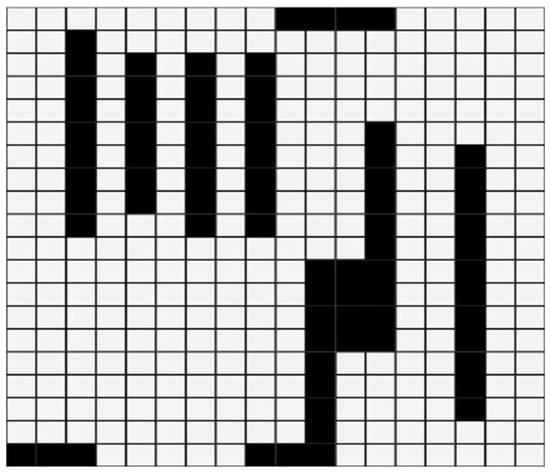
Figure 3.
Raster simulation diagram.
3.2. Coding Method
In path planning, the chromosome of the genetic algorithm is a feasible path from the start point to the goal point. To better represent the path information of the AGV, a variable-length symbolic code is used to encode the chromosome, and each gene in the chromosome corresponds to a raster number in the raster map. To ensure the feasibility and efficiency of the path, no obstacle number or duplicate number is allowed in the chromosome. In order to speed up the convergence of the genetic algorithm, we did not encode all the white rasters in Figure 3—only the rasters where special nodes, such as cargo containers and workstations, are located.
The encoded raster map is shown in Figure 4:
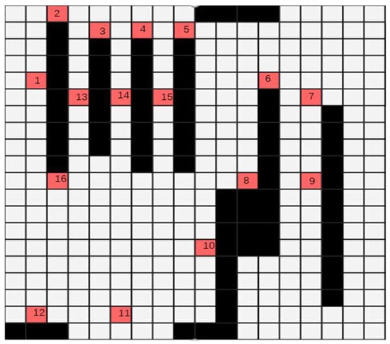
Figure 4.
Raster diagram with workstation nodes.
3.3. Optimization of the Fitness Function
In order to fully consider the effects of real road conditions and multiple AGVs, we use path smoothing factor and node busy factor to optimize the fitness function of the traditional genetic algorithm. Nodes refer to the orange raster in Figure 4.
3.3.1. Path Smoothing Factor
Because most AGVs use pulleys, they cannot complete turns with too much curvature at high speeds, so we use the path smoothing factor to reduce the number of turns of the AGV or to select turns with smaller angles. We calculate the path smoothing factor according to the number of turns and the turning angle of the AGV.
We calculate the path smoothing factor according to the time it takes for the AGV to complete the turn. The path smoothing coefficient is calculated as follows:
First, assume that the bends of the AGV working environment are complete quarter circles; the AGV turning time is calculated with the following formula:
where denotes the time taken, denotes the number of turns to be taken to reach point , is the turning speed, and is the radius of the turn.
Then, in order to be able to choose a smaller number of turns, we introduce the penalty factor ().
where represents the average speed, is the turning speed, is the radius of the turn, is number of turns, and is the penalty factor.
3.3.2. Node Busy Factor
The node busy factor avoids congestion of multiple AGVs. We first design a node usage table, as shown in Table 3, which indicates the number of times the current node will be passed by AGVs and the number of times AGVs are working or will work at the current node in a given time period (). Nodes can be further penalized with high hotness values to the extent that the paths that are about to be planned can be constrained by the paths that have been planned to achieve the goal of avoiding congestion of multiple AGVs. In addition to the number of tasks and the number of AGVs that affect the node congestion coefficient, AGVs starting the K-L algorithm to avoid dynamic obstacles affects the congestion coefficient of the nearest nodes to the AGVs through parameter so that the nodes can sense the presence of dynamic obstacles and improve the real-time performance of the algorithm.

Table 3.
Parameters of the K-L Algorithm.
The formula for calculating the node busy factor is as follows:
where is the node number, is the used node number, set indicates the number of times the current node has been worked or will be worked by the AGVs, set indicates the number of times the current node will be passed by the AGVs, is the total number of AGVs, denotes the busy factor of node , is the penalty factor of dynamic obstacles, and is the number of dynamic obstacles that appear.
3.3.3. Weight-Based Polling Algorithm
The sum of the current node’s busy factor is greater than the maximum value, and the outgoing AGVs will be suspended and enter the queuing session. Next, we calculate the weight of each AGV in the queue according to three dimensions: waiting time, task distance, and the performance level of the AGVs. The calculation formula is as follows:
where is a normalization function; is the time reward parameter, which is used to increase the weight of AGVs with long waiting times; is the waiting time; is the task linear distance; and is the rank of AGVs, with a maximum rank of 3 and a minimum rank of 1.
Then, we propose a weight-based smoothing polling algorithm (Algorithm 1), which rationalizes the departure order of AGVs according to their weights. The specific algorithm is as follows:
| Algorithm 1 Weight-based smoothing polling algorithm. |
| WBSP Procedure |
| Input: Number of AGVs in waiting status , AGVs current set of weights , AGVs fixed set of weights , and Serial number of the best AGVs Best. |
| Output:Best |
| for each AGVs |
| Initialize the current weight of AGVs, = 0 |
| Calculating the fixed weights of AGVs |
| end for |
| , |
| while n < |
| Random selection of an AGVs |
| = + |
| if < |
| n = n + 1; |
| end while |
| print Best |
| end procedure |
Based on the above algorithm, we can prioritize the AGVs based on the weight size. When AGVs are unable to depart due to peak congestion factor or for other reasons, they can be selected again according to the polling mechanism.
The Final Fitness Function Is Calculated as Follows
where and are the node busy factor and path smoothing factor, respectively; and denotes the straight-line distance between node and node .
According to Equations (9)–(12), with fewer turns, the turn angle is smaller, and the node heat value is lower, resulting in a smaller value. According to the wheel selection mechanism of the genetic algorithm, it is easy to obtain paths with small values, thus preventing the algorithm from selecting paths with too many turns or paths prone to congestion.
4. Two-Level Path Planning Method
The K-L algorithm is similar to other local path planning algorithms, which achieve obstacle avoidance and pathfinding of dynamic obstacles by sacrificing time; however, if the whole process is accomplished only using only the K-L algorithm, it will considerably reduce the transportation efficiency of AGVs. Therefore, the area where the K-L algorithm is used needs to be as small as possible, in addition to a reasonable timing requirement to maximize the advantages of the algorithm. In this paper, we first use the improved genetic algorithm to obtain the global path; then, when the AGV’s radar detects an obstacle that cannot be avoided, we use the K-L algorithm to complete obstacle avoidance in a limited area. In addition, because the dynamic working environment is generally narrow, if there is no reasonable scheduling method, considerable congestion of multiple AGVs will occur, reducing the transportation efficiency of AGVs. In this paper, the scheduling of multiple AGVs can be accomplished through the node busy factor. In other words, AGVs can avoid the more congested nodes by detouring, which maximizes the transportation efficiency of multiple AGVs.
The GA-KL method flow is shown in Figure 5. The main steps of a two-level path planning method combining the K-L algorithm and an improved genetic algorithm are as follows:

Figure 5.
Flow chart of the GA-KL method.
- (1)
- The working environment is scanned by the AGV’s own SLAM system, which obtains map information to create a raster map.
- (2)
- First, the optimal set of global path nodes is obtained using the T-GA algorithm; then, the shortest path between nodes is generated using the A* algorithm, and the algorithm aims at the shortest path length.
- (3)
- Due to the global set of path nodes, we divide the whole path into multiple subpaths to obtain multiple local target points.
- (4)
- For each subpath, we first detect dynamic obstacles using the detection radar of the AGV; then, when dynamic obstacles appear, the K-L algorithm is enabled to complete obstacle avoidance and select the shortest path length as the goal to obtain the local optimal path; if there are no obstacles, the path planned by the A* algorithm continues to be used.
5. Experimental Results and Discussion
5.1. Parameter Settings
For the following experiments, the parameters used by the algorithm are specified in Table 4 and Table 5.

Table 4.
Parameters of the K-L algorithm.

Table 5.
Parameters of the GA-KL method.
The total number of training sessions is 1500, and the maximum number of iterations per training session is 1000.
5.2. Experiment 1: Experiments to Verify the Effectiveness of the K-L Algorithm
This experiment is carried out to prove the effectiveness of the K-L algorithm according to the AGVs driving path and Q-value curve during the training process. The experiment uses a 10 × 10 raster map, as shown in Figure 6. The starting point is located in the lower-left corner of the map, and the end point is in the upper-right corner of the map. The obstacles are randomly placed inside the map, as represented by black raster. The AGV uses the K-L algorithm to accomplish the path optimization task. If the AGV collides with an obstacle, it immediately returns to the original position to speed up the training.
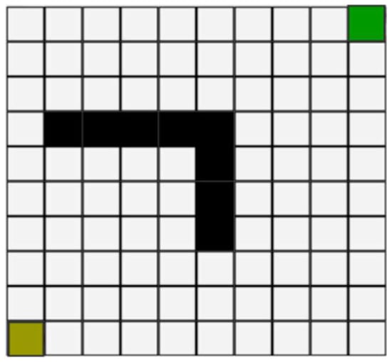
Figure 6.
Raster map. The yellow raster is the starting point, and the green raster is the ending point.
As shown in Figure 7, the green raster represents the path that the AGV travels during the training process. Figure 7a–d show the results of the 256th, 644th, 960th, and 1445th training iteration, respectively. As shown in Figure 7a, because the training process is in the early stage, the probability of exploration is high, so the AGV can easily collide with the obstacle. However, as the number of training sessions increases, the K-L algorithm accumulates more experience with the environment, and the AGV is eventually able to avoid obstacles, as shown in Figure 7b–d.
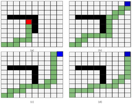
Figure 7.
AGV roadmap. The red grid represents not reaching the end point, and the blue grid means reaching the end point successfully. (a–d) represent the trajectories at different numbers of iterations, respectively.
Figure 8 shows the average Q-values of K-L for every 100 iterations. (a), (b), (c), and (d) in Figure 7 correspond to curves (a), (b), (c), and (d) in Figure 8, respectively. The path lengths of curves (a), (b), (c), and (d) are 10 m, 24 m, 20 m, and 19 m, respectively. Except for curve (a), as the training progresses, the path lengths of each curve gradually decrease, which proves that the K-L algorithm is converging to a better solution. As for curve (a), because the AGV collides with the obstacle and returns to the starting point, the path length of curve (a) remains constant at 10. A comparison of Figure 7 and Figure 8 shows that when the AGV collides with an obstacle far away from the end point, the Q-value will continue to decrease until it is 0; when the AGV bypasses the obstacle and reaches the end point, the Q-value continues to increase and remains stable in later training stages.
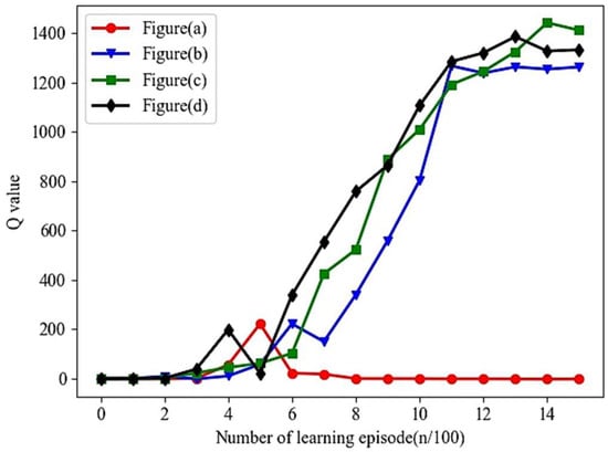
Figure 8.
Q-value curve.
5.3. Experiment 2: Comparison of the Convergence Time of K-L Algorithm and the Improved Q-Learning Algorithm
With the same raster maps and the same start point and end point, we compare the K-L algorithm with two representative improved Q-learning algorithms: the path-integral-based reinforcement learning algorithm (PIRL) [23] and a hybrid A* algorithm with reinforcement learning (HARL) [24]. The maps used for the experiments are 30 × 30 and 40 × 40 raster maps, respectively. In the experiment, a dynamic obstacle is randomly generated in order to demonstrate that the K-L algorithm converges well in different environments.
As shown in Table 6 and Table 7, 30 × 30 and 40 × 40 raster maps are used in the experiment, with randomly placed obstacles. Based on the number of states that, although the map has changed, the K-L algorithm still reduces the number of states by adaptive clustering, leading to faster convergence compared to PIRL and HARL. Because PIRL achieves path optimization according to an a priori knowledge base, its convergence slows down because the larger the map, the more states and less prior knowledge. HARL is a length-first best path algorithm based on the A* algorithm and prior knowledge RL strategy, so similarly, it converged slowly due to a lack of prior knowledge.

Table 6.
Time of convergence and the number of states in a 30 × 30 raster map.

Table 7.
Time of convergence and the number of states in a 40 × 40 raster map.
5.4. Experiment 3: Comparison of the Convergence Time of K-L Algorithm and Q-Learning Algorithm Based on Clustering Network Improvement
To further verify the advantages of the K-L algorithm with respect to convergence speed, we compared the K-L algorithm with two reinforcement learning algorithms based on the clustering network: AHC [13] and the K-means clustering-based reinforcement learning algorithm (KML) [25]. The convergence curve of the path length on a 20 × 20 raster map is shown in Figure 9.
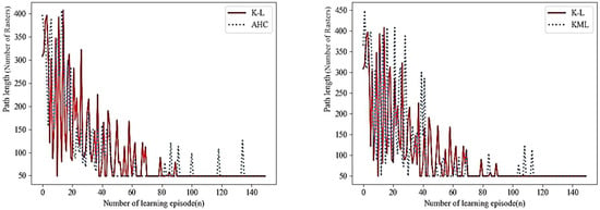
Figure 9.
Comparison chart of K-L algorithm in convergence time.
Figure 9 shows the difference in convergence speed of the three reinforcement learning algorithms. K-L converges after approximately 90 episodes, whereas AHC converges after approximately 122 episodes, and KML begins to converge after approximately 115 episodes. The number of states of K-L is 1500, whereas the number of states of AHC is 1631, and the number of states of KML is as high as 2074, mainly because rather than using hierarchical clustering like AHC and KML, K-L accomplishes clustering by self-competition, which speeds up the convergence by dynamically adjusting parameters. Furthermore, the K-L algorithm does not send any fluctuations after 90 iterations, which proves that the K-L algorithm has good stability.
5.5. Experiment 4: Comparing the Impact of Different Exploration Strategies on the K-L Algorithm
To further validate the advantages of the K-L algorithm in exploring strategies, using the same area with the same start point and end point, we compare the SSA exploration strategies of the K-L algorithm with different representative strategies, including the -decreasing strategy [24], the action selection strategy [15], and the traditional -greedy strategy. As shown in Figure 10, three raster maps are used in the experiments, sized 10 × 10, 20 × 20, and 30 × 30, with randomly placed static obstacles, as well as a dynamic obstacle. The dynamic obstacle moves back and forth between the upper raster and the lower raster of its starting position. The average results of path lengths and convergence times of 1500 repeated experiments are shown in Figure 11 and Figure 12.
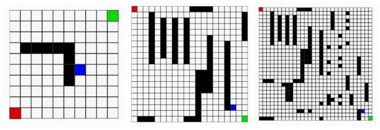
Figure 10.
Raster maps. The red raster is the starting point, the green raster is the ending point, the black raster is the static obstacle, and the blue raster is the dynamic obstacle.
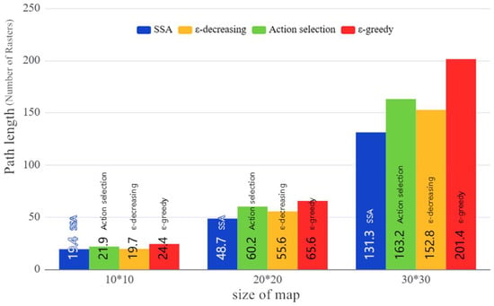
Figure 11.
Path length comparison chart.
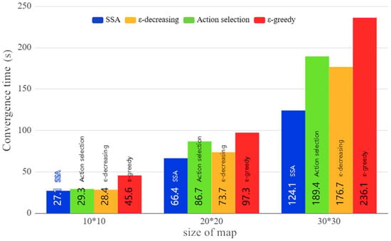
Figure 12.
Comparison chart of SSA in convergence time.
As shown in Figure 11, the exploration strategy based on the SSA achieves better results in terms of path length, followed by the -decreasing strategy, action selection strategy, and -greedy strategy. Because the -decreasing strategy is based on linear changes, it cannot be adjusted dynamically according to the current situation, so it is poorly optimized against dynamic obstacles. On the other hand, the action selection strategy is only good at avoiding dynamic obstacles, whereas the SSA strategy is not easily affected by map changes due to its ability to adaptively adjust.
Figure 12 shows that SSA has an advantage in terms of convergence time. The -decreasing strategy is the fastest among the investigated strategies, followed by the action selection strategy and the -greedy strategy. Because SSA is dynamically adaptive, it can effectively balance exploration and utilization as the map changes; as a result, the K-L algorithm converges quickly and can find the optimal path with high probability.
5.6. Experiment 5: Experiments Based on GA-KL Path Planning Method for Real Environments
To verify the global path planning effect and obstacle avoidance capability of the GA-KL method, we built a real factory environment, which includes workstations, charging piles, office chairs, multi-AGVs, and staff. The experimental environment is shown in Figure 13.
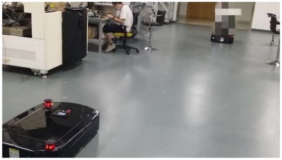
Figure 13.
Experimental scene.
We define workstations and charging posts as nodes and office chairs and walls as obstacles and use MapControl (MapControl is a mapping tool) to draw a scene map. The scene map is shown in Figure 14.
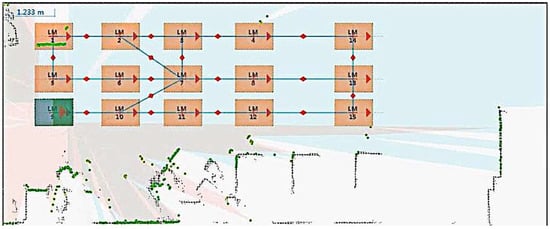
Figure 14.
The scene map.
To verify the global path planning capability of the method, we use a worker as a dynamic obstacle, who keeps moving back and forth between node 2 and node 3 to increase the node busy factor of node 3. Based on the above design, we use dynamic frontal collision experiments and dynamic side collision experiments to verify the obstacle avoidance capability of the GA-KL method. The above design is also designed to restore the working environment of real AGVs and to verify the effectiveness of the GA-KL method more realistically.
5.6.1. Experiments on Frontal Avoidance of Dynamic Obstacles by AGVs Based on the GA-KL Method
First, the AGV with serial number A receives a task from node 8 to node 1. As shown in Figure 15, the AGV can complete the task either through the (8-7-6-5-1) or through the (8-7-2-1). In terms of distance, (8-7-2-1) < (8-7-6-5-1), but the staff moves back and forth from node 2 to node 3, increasing the node busy factor of node 2, resulting in a larger -value according to Equation (13). According to the roulette selection method, the T-GA algorithm chooses (8-7-6-5-1) with a longer distance but relatively small value. When the AGV with sequence number A arrives at node 7, the AGV with sequence number B departs from node 5 to node 7. At this time, the detection radar of the AGV with serial number A has already detected the AGV with serial number B, so it immediately uses the K-L algorithm to plan the local path and successfully achieves avoidance.

Figure 15.
Frontal avoidance. A and B are the serial numbers of AGVs respectively.
5.6.2. Experiments on Side Avoidance of Dynamic Obstacles by AGVs Based on the GA-KL Method
As shown in Figure 16, the AGV with sequence number A receives a task from node 1 to node 8, and its global path is (1-2-7-8). When the AGV with sequence number A reaches node 2, the AGV with sequence number B departs from node 8 to node 1, and its global path is (8-7-6-5-1). At this time, the detection radar of the AGV with sequence number B has detected the AGV with sequence number A, so it immediately uses the K-L algorithm to plan the local path. At this point, if the K-L algorithm selects the AGV upward avoidance, which is blocked by the staff at node 3, the algorithm selects downward avoidance and successfully returns to node 6.

Figure 16.
Side avoidance. A and B are the serial numbers of AGVs respectively.
5.7. Experiment 6: GA-KL Method Stability Test in a Narrow Operating Environment
To further verify that the GA-KL method can improve the efficiency of AGVs in a narrow operating environment, we compare the GA-KL method with four path planning methods: a three-layer control model-based path planning method [19] (referred to as GP-AP), a BP neural network-based path planning method (referred to as BP-P) [20], a path integral-based reinforcement learning algorithm [23] (PIRL), and a hybrid A* algorithm with a reinforcement learning path planning approach (HARL) [24]. We carried out five path planning experiments in real life with the same start point and end point. As shown in Figure 17, the field experiment environment consists of obstacles (another AGV) and walls. The experimental results are shown in Table 8.
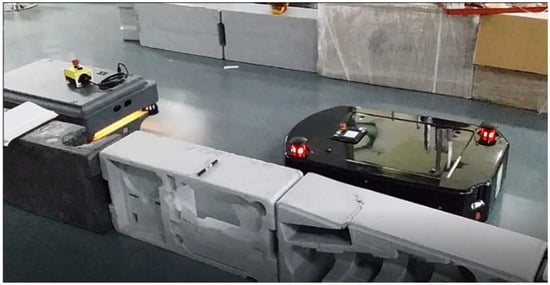
Figure 17.
Environment of the field experiment. The field experiment parameters are as follows.

Table 8.
Run time and path length for five rounds of path planning.
- (1)
- Size of the map: 20 m × 10 m.
- (2)
- Coordinates of starting point: (−9.50 m, 5.87 m); coordinates of target point: (6.25 m, 1.83 m).
- (3)
- Average speed of AGVs: 0.8 m/s.
As shown in Table 8, comparing the GP-AP and BP-P path planning methods based on neural network reinforcement, although the path length of the GA-KL method is longer, the running time is much shorter than that of the other two methods. Comparing the hybrid path planning methods of HARL and PIRL, the GA-KL method achieves satisfactory results in terms of path length and running time because the GA-KL algorithm can coordinate the path of the two AGVs in advance according to the node busy factor, whereas the remaining two methods start their own obstacle avoidance algorithms to achieve avoidance, which wastes time, considerably reducing the efficiency. In a real factory environment, we want the total working time of multi-AGVs to be as short as possible, so the GA-KL method is most suitable for a real factory environment.
5.8. Experiment 7: GA-KL Method Stability Test in a Highly Congested Environment
To further verify the advantages of the GA-KL method in a highly congested environment, we compare the GA-KL method with three path planning methods: a path integral-based reinforcement learning algorithm [23] (PIRL), a hybrid A* algorithm with a reinforcement learning path planning approach (HARL) [24], and a multi-destination path planning method [26] (OSPC). Figure 15 shows the map used for the experiments; sequence number 13 is the starting point, and the rest of the sequence numbers are the destination points. We used five AGVs departing simultaneously and conducted five multi-AGV path planning experiments, in which the starting point of each AGVs is the same, but the target point is randomized. Each time an AGV reaches the target point, it automatically accepts the task of returning from the target point to the starting point. Dynamic obstacles randomly appear between the nodes, and the number of dynamic obstacles gradually increases. Such an experimental design is associated with a high probability of congestion; the purpose is to test the performance of each path planning method under congestion conditions. The experimental results are shown in Figure 18 and Figure 19.
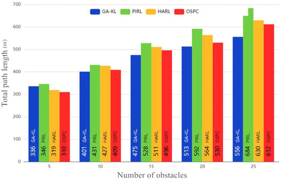
Figure 18.
Comparison of total path length.
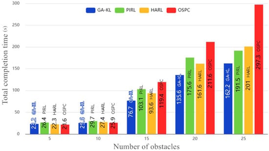
Figure 19.
Comparison of total completion time.
As shown in Figure 18 and Figure 19, the GA-KL algorithm achieves better results in terms of total path length and total completion time as the number of dynamic obstacles increases. PIRL achieves path optimization through an a priori knowledge base, but the AGVs depart simultaneously, meaning the a priori knowledge obtained from each AGV cannot be shared, with a lack of a scheduling function; therefore, the planning results degenerate as the number of dynamic obstacles increases. For HARL, although the A* algorithm provides a satisfactory global search capability, it suffers from the same problems as PIRL, i.e., a lack of sharing of prior knowledge and a lack of scheduling capability. For OSPC, although its multi-purpose path planning provides advantages in terms of total path length, it is a static algorithm that does not have the ability to handle congestion and dynamic obstacles when they occur. GA-KL does not need to share a priori knowledge but achieves scheduling with an improved genetic algorithm, and the appearance of dynamic obstacles is fed back to the node congestion coefficient in time; when the node congestion coefficient reaches a certain peak, it suspends the departing AGVs into a queuing session to reduce the risk of congestion as much as possible, achieving satisfactory performance with respect to total completion time.
6. Conclusions
In order to improve the transportation efficiency of multi-AGVs in dynamic and special environments, an improved Q-learning path optimization algorithm based on a Kohonen network (K-L) is proposed, and a two-level path planning method is proposed by combining the K-L algorithm with an improved genetic algorithm (GA-KL).
The results of this study are as follows:
- (1)
- The K-L algorithm introduces an exploration strategy of an adaptive simulated annealing algorithm and the Kohonen network state classification method, as well as an improved reward function based on potential energy, which can effectively handle path planning in complex environments with fast convergence and satisfactory optimization results. Through simulation and field experiments, the effectiveness of the K-L algorithm is further verified; the convergence time of the algorithm is reduced by about 6.3%, on average, and the path length of AGVs is reduced by about 4.6%, on average.
- (2)
- The GA-KL method uses the T-GA algorithm for global path planning and the K-L algorithm for local path planning. The T-GA algorithm is a genetic algorithm optimized by path smoothing coefficients and node busy coefficients, which can coordinate the path planning of multi-AGVs and make the AGVs complete their tasks as soon as possible. In addition, the GA-KL method integrates a scheduling policy into global path planning, which can obtain a better dynamic scheduling policy for multi-AGVs in different environments and under different congestion conditions. Finally, it is experimentally demonstrated that the GA-KL method reduces the total path length by 8.4%, on average, and the total path completion time by 12.6%, on average, compared to other path planning methods.
In future studies, we will continue to improve the scheduling method. Based on the task value, working time, and other factors, as well as the weight-based polling algorithm, we will design a multi-task assignment and scheduling method based on time windows.
Author Contributions
Conceptualization, Y.J.; methodology, Y.B.; validation, X.D.; formal analysis, D.H.; writing—original draft preparation, Y.B.; writing—review and editing, Y.J.; supervision, D.H. and Y.J. All authors have read and agreed to the published version of the manuscript.
Funding
This work was supported by the National Key R&D Program of China (grant numbers 2020YFB1707900 and 2020YFB1711800).
Institutional Review Board Statement
Not applicable.
Informed Consent Statement
Not applicable.
Data Availability Statement
Not applicable.
Conflicts of Interest
The authors declare no conflict of interest.
References
- Ajeil, F.H.; Ibraheem, I.K.; Azar, A.T.; Humaidi, A.J. Grid-based Mobile Robot Path Planning Using aging-based ant colony optimization algorithm in static and dynamic environments. Sensors 2020, 20, 1880. [Google Scholar] [CrossRef] [PubMed]
- Luo, Y.; Lu, J.; Zhang, Y.; Qin, Q.; Liu, Y. 3D JPS Path Optimization Algorithm and Dynamic-Obstacle Avoidance Design Based on Near-Ground Search Drone. Appl. Sci. 2022, 12, 7333. [Google Scholar] [CrossRef]
- Liang, D.; Liu, Z.; Bhamara, R. Collaborative Multi-Robot Formation Control and Global Path Optimization. Appl. Sci. 2022, 12, 7046. [Google Scholar] [CrossRef]
- Nazarahari, M.; Khanmirza, E.; Doostie, S. Multi-objective multi-robot path planning in continuous environment using an enhanced genetic algorithm. Expert Syst. Appl. 2019, 115, 106–120. [Google Scholar] [CrossRef]
- Duan, H.; Yu, Y.; Zhang, X.; Shao, S. Three-dimension path planning for UCAV using hybrid meta-heuristic ACO-DE algorithm. Simul. Model. Pract. Theory 2010, 8, 1104–1115. [Google Scholar] [CrossRef]
- Ahmed, F.; Deb, K. Multi-objective optimal path planning using elitist non-dominated sorting genetic algorithms. Soft Comput. 2013, 7, 1283–1299. [Google Scholar] [CrossRef]
- Wang, S.F.; Zhang, J.X.; Zhang, J.Y. Artificial potential field algorithm for path control of unmanned ground vehicles formation in highway. Electron. Lett. 2018, 54, 1166–1167. [Google Scholar] [CrossRef]
- Tian, W.J.; Zhou, H.; Gao, M.J. A path planning algorithm for mobile robot based on combined fuzzy and Artificial Potential Field. In Advanced Computer Technology, New Education, Proceedings; Xiamen University Press: Wuhan, China, 2007; pp. 55–58. [Google Scholar]
- Sun, Y.; Zhang, R.B. Research on Global Path Planning for AUV Based on GA. Mech. Eng. Technol. 2012, 125, 311–318. [Google Scholar]
- Ahmed, N.; Pawase, C.J.; Chang, K. Distributed 3-D Path Planning for Multi-UAVs with Full Area Surveillance Based on Particle Swarm Optimization. Appl. Sci. 2021, 11, 3417. [Google Scholar] [CrossRef]
- Xu, L.H.; Xia, X.H.; Luo, Q. The study of reinforcement learning for traffic self-adaptive control under multiagent markov game environment. Math. Probl. Eng. 2013, 2013, 962869. [Google Scholar] [CrossRef]
- Yung, N.C.; Ye, C. An intelligent mobile vehicle navigator based on fuzzy logic and reinforcement learning. IEEE Trans. Syst. Man Cybernetics. Part B Cybern. 1999, 29, 314–321. [Google Scholar] [CrossRef] [PubMed]
- Hengst, B. Discovering Hierarchical Reinforcement Learning, Sydney; University of New South Wales: Sydney, NSW, Australia, 2008. [Google Scholar]
- Xie, R.; Meng, Z.; Zhou, Y.; Ma, Y.; Wu, Z. Heuristic Q-learning based on experience replay for three-dimensional path planning of the unmanned aerial vehicle. Sci. Prog. 2020, 103, 0036850419879024. [Google Scholar] [CrossRef] [PubMed]
- Osowski, S.; Szmurlo, R.; Siwek, K.; Ciechulski, T. Neural Approaches to Short-Time Load Forecasting in Power Systems—A Comparative Study. Energies 2022, 15, 3265. [Google Scholar] [CrossRef]
- Souza, L.C.; Pimentel, B.A.; Filho, T.D.M.S.; de Souza, R.M. Kohonen map-wise regression applied to interval data. Knowl. Based Syst. 2021, 224, 107091. [Google Scholar] [CrossRef]
- Moskalev, A.K.; Petrunina, A.E.; Tsygankov, N.S. Neural network modelling for determining the priority areas of regional development. IOP Conf. Ser. Mater. Sci. Eng. 2020, 986, 012–017. [Google Scholar] [CrossRef]
- Shneier, M.; Chang, T.; Hong, T.; Shackleford, W.; Bostelman, R.; Albus, J.S. Learning traversability models for autonomous mobile vehicles. Auton. Robots 2008, 24, 69–86. [Google Scholar] [CrossRef]
- Na, Y.-K.; Oh, S.-Y. Hybrid Control for Autonomous Mobile Robot Navigation Using Neural Network Based Behavior Modules and Environment Classification. Auton. Robots 2003, 15, 193–206. [Google Scholar] [CrossRef]
- Griepentrog, H.W.; Jaeger, C.L.D.; Paraforos, D.S. Robots for Field Operations with Comprehensive Multilayer Control. KI Künstliche Intell. 2013, 27, 325–333. [Google Scholar] [CrossRef][Green Version]
- Dou, J.; Chen, C.; Pei, Y. Genetic Scheduling and Reinforcement Learning in Multirobot Systems for Intelligent Warehouses. Math. Probl. Eng. Theory Methods Appl. 2015, 25, 597956. [Google Scholar] [CrossRef]
- Cui, W.; Wang, H.; Jan, B. Simulation Design of AGVS Operating Process in Manufacturing Workshop. In Proceedings of the 2019 34rd Youth Academic Annual Conference of Chinese Association of Automation (YAC), Jinzhou, China, 6–8 June 2019; pp. 6–10. [Google Scholar] [CrossRef]
- Yongqiang, Q.; Hailan, Y.; Dan, R.; Yi, K.; Dongchen, L.; Chunyang, L.; Xiaoting, L. Path-Integral-Based Reinforcement Learning Algorithm for Goal-Directed Locomotion of Snake-Shaped Robot. Discret. Dyn. Nat. Soc. 2021, 12, 8824377. [Google Scholar] [CrossRef]
- Liu, X.; Zhang, D.; Zhang, T.; Cui, Y.; Chen, L.; Liu, S. Novel best path selection approach based on hybrid improved A* algorithm and reinforcement learning. Appl. Intell. 2021, 51, 9015–9029. [Google Scholar] [CrossRef]
- Guo, X.; Zhai, Y. K-Means Clustering Based Reinforcement Learning Algorithm for Automatic Control in Robots. Int. J. Simul. Syst. 2016, 17, 24–30. [Google Scholar]
- Zhuang, H.; Dong, K.; Qi, Y.; Wang, N.; Dong, L. Multi-Destination Path Planning Method Research of Mobile Robots Based on Goal of Passing through the Fewest Obstacles. Appl. Sci. 2021, 11, 7378. [Google Scholar] [CrossRef]
Publisher’s Note: MDPI stays neutral with regard to jurisdictional claims in published maps and institutional affiliations. |
© 2022 by the authors. Licensee MDPI, Basel, Switzerland. This article is an open access article distributed under the terms and conditions of the Creative Commons Attribution (CC BY) license (https://creativecommons.org/licenses/by/4.0/).