Multifunctional Models, Including an Artificial Neural Network, to Predict the Compressive Strength of Self-Compacting Concrete

Abstract

In this study, three different models were developed to predict the compressive strength of SCC, including the nonlinear relationship (NLR) model, multiregression model (MLR), and artificial neural network. Thus, a set of 400 data were collected and analyzed to evaluate the effect of seven variables that have a direct impact on the CS, such as water to cement ratio (w/c), cement content (C, kg/m³), gravel content (G, kg/m³), sand content (S, kg/m³), fly ash content, (FA, kg/m³), superplasticizer content (SP, kg/m³), and curing time (t, days) up to 365 days. Several statistical assessment parameters, such as the coefficient of determination (R²), root mean squared error (RMSE), mean absolute error (MAE), and scatter index (SI), were used to assess the performance of the predicted models. Depending on the statistical analysis, the median percentage of superplasticizers for the production of SCC was 1.33%. Furthermore, the percentage of fly ash inside all mixes ranged from 0 to 100%, with 1 to 365 days of curing and sand content ranging from 845 to 1066 kg/m³. The results indicated that ANN performed better than other models with the lowest SI values. Curing time has the most impact on forecasts for the CS of SCC modified with FA.

1. Introduction

Self-consolidating concrete or self-compacting concrete (SCC) is a concrete mix that has low yield stress, high deformability, good segregation resistance (prevents separation of particles in the mix), and moderate viscosity (necessary to ensure uniform suspension of solid particles during transportation, placement (without external compaction), and until the concrete sets). In everyday terms, when poured, SCC is an extremely fluid mix with the following distinctive practical features: it flows very easily within and around the formwork, can flow through obstructions and around corners (“passing ability”), is close to self-leveling (although not self-leveling), does not require vibration or tamping after pouring, and follows the shape and surface texture of a mold (or form) very closely once set. As a result, pouring SCC is much less labor-intensive than standard concrete mixes. Once poured, SCC is usually similar to standard concrete in terms of its setting and curing time (gaining strength) and strength. SCC does not require a high proportion of water to become fluid and SCC may contain less water than standard concretes. Instead, SCC gains its fluid properties from an unusually high proportion of fine aggregate, such as sand (typically 50%), combined with superplasticizers (additives that ensure particles disperse and do not settle in the fluid mix) and viscosity-enhancing admixtures (VEAs) [1,2]. The introduction of SCC represents a major technological advance, leading to a better quality of concrete produced and a faster and more economical concrete construction process [3]. When there is a lot of reinforcement in the structure members, using an SCC is the perfect choice for structural components. A superplasticizer and other mineral admixtures can increase the SCC’s high flowability and stability [4].

Fly ash (FA) is a siliceous or aluminosilicate particle that has been finely divided. When moisture is present, it chemically combines with the calcium hydroxide generated when Portland cement hydrates to create a compound with cementing properties [5]. As a byproduct of burning pulverized coal, FA is a finely split residue produced in coal-fired power plants. The coal is crushed and blown into the burning chamber, where it burns right away to heat the boiler tubes. Regarding the influence of fly ash on self-compacting concrete (SCC) properties, a study indicates that a high volume of fly ash can be used in SCC to produce high-strength and low-shrinkage concrete. Subhan Ahmad et al. compared hardened properties of normal concrete (NC) and self-compacting concrete (SCC) [6]. While most of the impurities deposited in coal during its formation, such as clay, shale, quartz, and feldspar, typically fuse and stay suspended in the flue gas, the volatile matter and carbon are burned off. The importance of a low water–cement ratio for enhancing the durability of concrete has long been accepted. Low water content leads to low workability of the fresh concrete; if this concrete is not properly compacted, the durability of the structures will be impaired. In the mid-1970s, superplasticizers were introduced to the market to produce rhinoplastic concretes [7,8]. The flaming material is swiftly transferred to cooler regions, where it is formed into sphere-shaped particles. Lighter ash particles (FA) stay suspended in exhaust gases while heavier ash particles fall to the bottom of the burning chamber. Mechanical separators, electrostatic precipitators, or bag filters are used to remove these FA particles [9]. Previous research has shown that using mineral admixtures such as fly ash in concrete mixes can improve the slump without increasing expense while lowering the amount of superplasticizer needed to achieve equal slump flow when compared to concrete prepared only with Portland cement, and the presence of the fly ash lessens the heat of hydration and increases the durability [10]. Due to its finer and more rounded particles than cement, fly ash can be used to replace cement in the creation of self-compacting concrete. Fly ash could operate as a filler to cover the inter-particle spaces that cement is unable to occupy by making use of these physical features [11].

SCC consists of similar components to conventionally vibrated concrete: cement, aggregates, water, mineral, and chemical admixtures. The passing ability and segregation resistance of SCC are achieved by the decrease in coarse aggregate content and increases in the powder quantities. The superplasticizers (high-range water reducers) are responsible for the high fluidity of the concrete mix, while the powder and viscosity-modifying agents lead to better stability and cohesion, reducing bleeding and segregation of the mix.

Mineral admixtures are used as extra-fine material; the most used is the limestone filler which represents a chemically inert by-product of limestone crushers. The addition of limestone powder improves the particle packing by filling the small pores between cement grains and augmenting the water retention of fresh mixes. The compressive strength is calculated by the failure load divided by the cross-sectional area resisting the load and reported megapascals (MPa). Concrete hardens and acquires strength as it hydrates. This process occurs rapidly at first and slows down as time goes by; it continues over a long period.. This study investigated the compressive strength at 28 days, an age considered for design purposes when a substantial percentage of hydration has taken place. The cube and cylinder strength of SCC and conventional vibrated concrete was determined at the same w/c ratio and cement content [12,13]. To ascertain the compressive strength of SCC modified with FA, several cylindrical or cubical specimens are currently produced and tested over various curing times in the practice field. Generally speaking, work on the construction site should not continue until the results of the compressive strength test at a given age, particularly 28 days, are available. Due to this, testing takes longer than expected and is more expensive [14]. Construction sites are also delayed as a result. Fly ash can replace 40% of the cement in self-compacting concrete to increase its strength to 65 MPa [10]. The term “binder content” refers to the cement and any additional pozzolanic elements that may be included in the mixture to enhance specific SCC characteristics. FA is additionally one of the most reactive pozzolanic materials. With an increase in cement or binder content, the compressive strength of SCC was typically noticeably enhanced [4,15]. When the amount of cement was increased from 360 to 450 kg/m³ at the same water content, the compressive strength of SCC increased from 48 and 52 MPa to roughly 52 and 60 MPa at 28 and 90 days, respectively [16,17,18].

The w/c or w/b ratio, similar to normal concrete, is one of the key factors affecting the CS of SCC at different curing ages. Compared to regular concrete, SCC frequently has a lower w/b ratio. When the w/b ratio is lower, a higher percentage of cement and binder ingredients produces a higher CS and a more homogeneous matrix [4]. The w/c or w/b ratio, similar to normal concrete, is one of the key factors affecting the CS of SCC at different curing ages. Compared to normal concrete, SCC frequently has a lower w/b ratio. When the w/b ratio is lower, a higher proportion of cement and binder ingredients produces a higher CS and a more homogeneous matrix. When the w/b ratio was decreased from 0.45 to 0.35 up to 56 days of curing, the CS of SCC was significantly improved at all curing ages [19]. The w/b ratio affects the CS of regular concrete more so than it does the CS of SCC [20].

One of the main advantages SCC has over other special concrete varieties is that it does not need any special curing procedures. Similar to regular concrete, SCC is cured using the same procedure. According to earlier studies [4,21], the most crucial factor affecting the CS of SCC is the age of the concrete samples after the examination. Longer curing times produced better compressive strength for the same mix proportions because of the faster rate of hydration. The CS of SCC was increased from 13 MPa to 54 MPa by extending the curing time from one day to 28 days, as demonstrated by Corinaldesi and Moriconi [22]. According to Sahmaran et al. [23], the 7-day CS of SCC was 55.9 MPa. However, when the curing age of SCC was raised to 180 days, this value increased to 71 MPa. SP’s high cement and binder contents make it impossible to make SCC without it. The presence of SP improves workability. Although SP is added to SCC to enhance its rheology, different dosages can also affect compressive strength. The CS of SCC increased by 30% after 28 days of curing as the SP dosage increased from 5.5 kg/m³ to 8.25 kg/m³ [24]. Aggregates comprise 60 and 70 percent of SCC’s volume, significantly impacting the material’s rheological and hardened performance. Compared to conventional concrete, SCC typically contains less coarse material [4]. According to earlier studies, the CS of SCC was less affected by the fine aggregate content than the coarse aggregate content.

Additionally, compared to coarse aggregates with a maximum size of 10 mm, those with a maximum size of 20 mm had a higher CS of SCC [25]. Artificial neural networks have been widely used in many studies, such as predicting the piezoelectric effect of the plate of engineering structures in vibration and noise reduction. This study employed an artificial neural network (ANN) model to explore the piezoelectric patch size and thickness’s effect on a plate’s first-order natural frequency and displacement amplitude. With the finite element method (FEM), a rectangular plate actuated by a piezoelectric patch was analyzed with various patch sizes. The FEM data were later used to build an ANN model. The dynamic response of the plate was predicted by the ANN model and validated with FEM in terms of first-order natural frequency and displacement amplitude. Case studies showed that the ANN model could accurately predict both natural frequency and displacement amplitude with patch length, width, and thickness input. When the information of the ANN model was simplified to patch size and thickness or the patch’s volume, the accuracy worsened. The patch size and thickness’s influences on the first-order natural frequency were coupled, and the maximal and minimal values were predicted based on the ANN model. The purpose of this research is to develop and apply the artificial neural network (ANN) with an extreme learning machine (ELM) to forecast the gross domestic product (GDP) growth rate. The economic growth forecasting was analyzed based on the value of agriculture, manufacturing, industry, and services added to GDP. The results were compared with the ANN with the backpropagation (BP) learning approach since BP could be considered a conventional learning methodology. The reliability of the computational models was assessed based on simulation results and several statistical indicators. The results showed that the ANN with ELM learning methodology could be applied effectively in applications of GDP forecasting [23,24,25,26,27].

Since compressive strength depends on various characteristics and mixture proportions, more sophisticated methodologies should be used to lessen the need for laboratory experiments and provide engineers with more convenient tools and numerical equations for predicting experimental results. An excellent strategy is to use soft computing techniques. The main benefit of using these techniques is the development of workarounds and solutions for linear or nonlinear problems where mathematical models cannot readily show the relationship between the pertinent factors in the problem [27,28,29,30]. A methodical multiscale model was developed to calculate the CS of concrete made with significant amounts of fly ash [28]. Four hundred fifty different experimental datasets were used to create a model. M5P trees, linear, nonlinear, and multilogistic regression were developed as five distinct qualification modeling methods. It was concluded that the ANN, M5P tree, and multilogistic regression models could predict the CS of large-volume fly ash concrete wells based on higher R² and lower RMSE and MAE values [29].

Despite the wide use of FA in SCC mixes in the earlier studies, an accurate model could not be identified for effective use by the construction industry. As a result, it was attempted in this study to analyze and quantify the effects of a wide range of mixture proportions, including FA content, cement content, w/b ratio, SP content, fine aggregate content, and coarse aggregate content, on the CS of SCC up to 365 days of curing. Different model approaches, such as nonlinear regression, multiregression, and ANN models, were used to predict the CS of SCC modified by FA using 400 data samples from the literature. The main goals are to (i) conduct statistical analysis and assess how mixture compositions such as FA content, C content, G content, w/c ratio, SP content, and curing time affect the CS of SCC; (ii) examine and design a reliable model for estimating the CS among all models (NLR, MLR, and ANN models) using appropriate statistical measures; and (iii) reduce the overall cost by designing mixes with any necessary specifications without the need for trail mixes.

2. Materials and Methods

The collected data from various literature for this paper were 400; inserting all data into an Excel sheet, they were sorted into two groups. The largest group comprised two-thirds of the collected data and was named as the training dataset and used to develop the models. The other group, one-third of the dataset, was used to test the proposed models. As mentioned earlier, the main objective of this study is to design models to predict the compressive strength of SCC.

Table 1. Datasets used in the modeling process.

Ref.	Fly Ash, FA (%)	Cement (kg/m3)	Water/Cement Ratio (%)	Curing Time (Days)	Superplasticizer Content (%)	Fine Aggregate (kg/m3)	Coarse Aggregate (kg/m3)	Slump Flow Diameter (mm)	Compressive Strength (MPa)
[1]	0–40	365–468	0.4–0.6	14, 28, 56	2.2	803–918	778–879	652–772	35.7–69
[3]	35–90	183–317	0.38–0.72	7, 28, 90	0.2–1	476–1066	837	555–790	6.2–74.2
[5]	15–35	355–465	0.41–0.44	7, 28, 356	1.8–2	910	590	603–673	22.7–61.2
[28]	0–60	161–326	0.35–0.5	1, 7, 28	0.5–1.9	650–866	155–251	570–650	6.1–48.3
[31]	0–30	420–600	0.33–0.46	7, 28, 90	2	900	750	650–720	65.6–85.3
[32]	0–30	315–480	0.4, 0.45	7, 28	1.5–2.8	890	810	650–695	39–52
[33]	0–60	180–550	0.33, 0.44	7, 28, 91	1	640–890	780–924	600–806	9.6–77.5
[34]	0–55	225–500	0.35	3, 7, 28	1.5,1.6	908–967	652–694	630–700	40–78
[35]	50–70	221–369	0.29	7, 28, 90	2–3.33	579	703	650–780	10.4–27
[36]	-	160–280	0.33–0.42	1, 7, 28	0.1–0.6	808–1066	900	570–770	5–52
[37]	0–70	150–500	0.28–0.35	7–365	1.33	902–967	597–639	665–775	14.9–75.6
[38]	0–60	180–550	0.32, 0.44	28, 90	0.78–3	686–826	829–935	670–730	30–91.1
[39]	15–75	355–465	0.41–0.62	28–365	1.2–2	640–910	590	590–690	18–59.4
[40]	-	375	0.47	28	1	779–825	700–746	-	22.8–31.46
[41]	0–60	161–336	0.35–0.50	1, 7, 28	0.4–3.8	739–866	843–1118	570–650	4.9–48.3
[42]	60	180,450	0.37	1, 7, 28, 90	0.1–0.48	827–850	827–850	561	2.67–70.8
[43]	0–75	142–570	0.33	28	-	765–835	765–835	-	30–66
[44]	0–80	100–500	0.36	1, 7, 28, 56	0.7	751–874	876	657–712	4.55–84
[45]	-	310–622	0.38	28	0.56–1	780	720	-	38–59
[46]	0–100	115–539	0.33–0.72	7, 28, 90, 120	0.65–1.1	743	924	700–730	16–84.1
Remarks	Ranged from 0–100%	Ranged from 100–620 kg/m3	Varied from 0.28–0.72	Varied from 1–365 days	Ranged from 0.1–3.33%	Varied from 476–1024 kg/m3	Ranged from 590–1118 kg/m3	Varied from 561–806 mm	Ranged from 2.67–91.1 MPa

includes the detailed ranges and information about each variable studied in the paper, which was water to cement ratio (w/c), cement content (C, kg/m³), gravel content (G, kg/m³), sand content (S, kg/m³), fly ash content, (FA, kg/m³), superplasticizer content (SP, kg/m³), and curing time (t, days). All mentioned independent parameters were used to evaluate and estimate the compressive strength and compare the results with the measured strength. The procedure of the current study is simply designed in Figure 1.

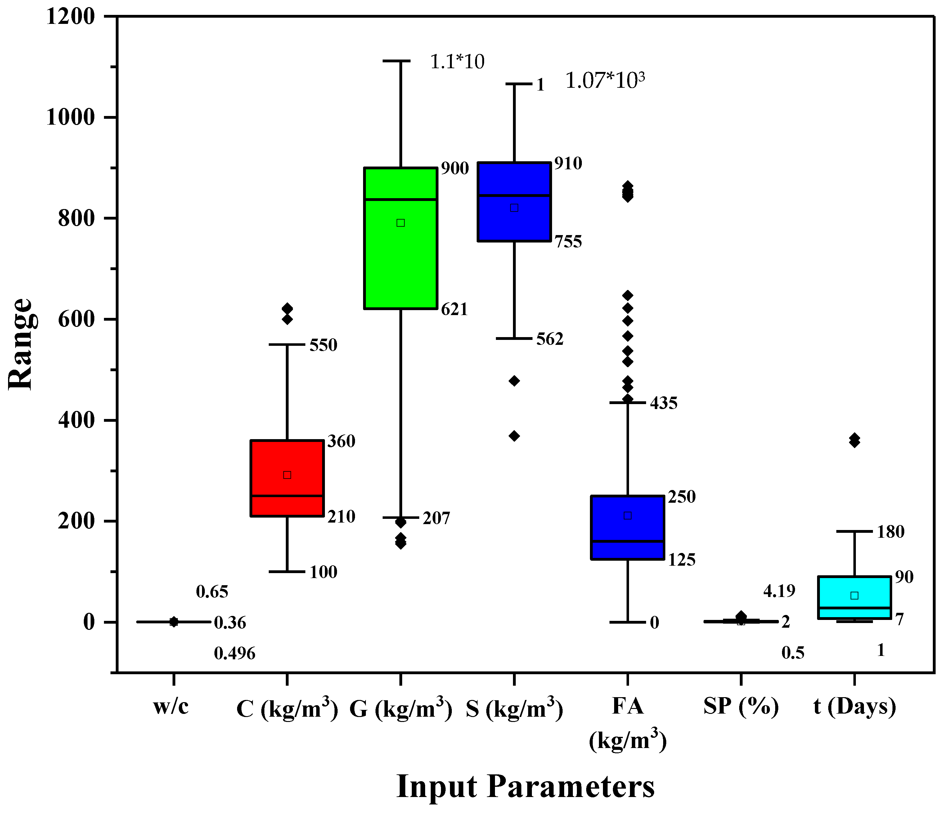
3. Statistical Evaluation

This part of the paper is about the statistical analysis of the dependent and independent variables separately to determine whether a strong relationship exists between each variable and the compressive strength of SCC modified with FA or not (Figure 2). Thus, the plot of all considered parameters, including water to cementitious material ratio, cement content, gravel content, sand content, fly ash content, superplasticizer content, and curing time with compressive strength, was prepared and analyzed (Figure 2, Figure 3 and Figure 4). The detail of the analysis results for each variable is explained as follows.

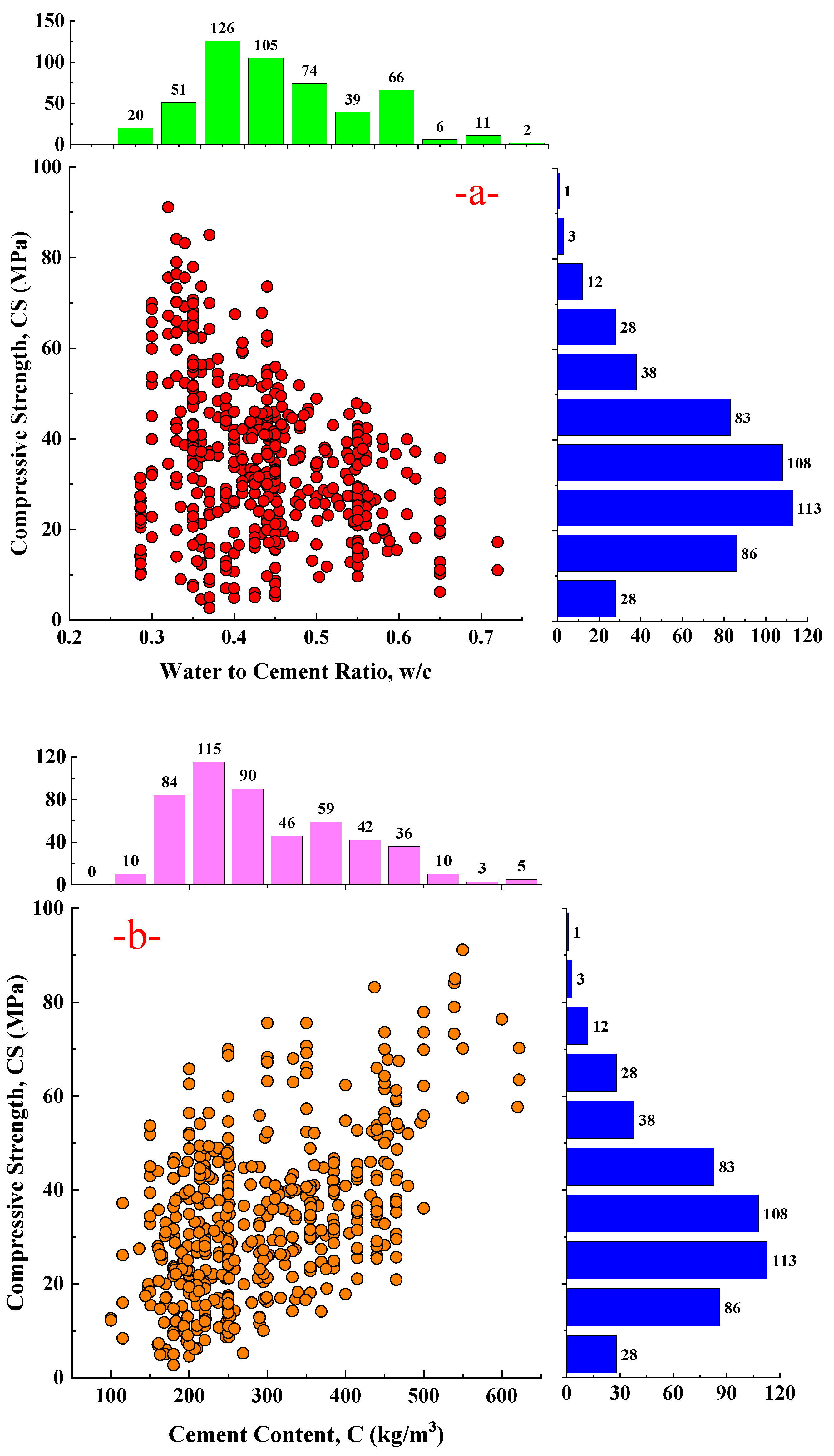
3.1. Water/Cement Ratio

The w/c ratio of SCC mixtures ranged from 0.28 to 0.72, with a median of 0.42, according to the total amount of data gathered. According to the statistical analysis, the other variables had the following values: 0.0075 for variance, 0.088 for standard deviation, 0.59 for skewness, and 0.24 for kurtosis. Figure 2 illustrates the connection between compressive strength and w/c ratio using the w/c ratio histogram (a) (

Table 2. The statistical analysis of the collected datasets.

Variable	St. Dev	Variance	Minimum	Median	Maximum	Skewness	Kurtosis
w/c	0.088	0.00775	0.28	0.42	0.72	0.59	−0.24
C, (kg/m3)	108.76	11,828.96	100	258	622	0.66	−0.35
G, (kg/m3)	196.06	38,441.25	590	837	1118	−1.20	2.21
S, (kg/m3)	106.3	11,298.6	476	845	1066	−0.93	1.18
FA, (kg/m3)	189.98	36,092	0	160	905	2.00	4.16
SP, (kg/m3)	1.461	2.1346	0	1.33	12.5	2.76	13.07
t, (days)	86.74	7524.2	1	28	365	2.69	6.73
CS, (MPa)	18.61	346.6	2.67	34.9	91.1	0.48	−0.38

).

3.2. Cement Content

According to the data gathered, the cement content of SCC mixtures ranged from 100 to 622 kg/m³, with a median value of 258 kg/m³. Based on the statistical analysis, the other variables had the following values: variance of 11,828.96, the standard deviation of 108.76, skewness of 0.66, and kurtosis of −0.35 (Figure 2b) (Table 2).

3.3. Gravel Content

Based on the total collected data, the SCC mixtures’ gravel content ranged from 590 to 1118, with an average of 837. The other variables’ values were as follows: variance of 38,441 standard deviation of 196.06.34, and skewness and kurtosis of −1.20 and −2.21, respectively. The relationship between compressive strength and gravel content with the histogram of gravel content is reported in Figure 2c (Table 2).

3.4. Sand Content

Sand content varied from 476 to 1066 kg/m³, with an average value of 845 kg/m³. According to the statistical analysis, the other variables had the following values: a variance of 11,298 a standard deviation of 106.3, and skewness and kurtosis values of −0.93 and 1.18, respectively (d) (Table 2).

3.5. FA Content

The FA content of SCC mixtures ranged from 0 to 905 kg/m³, with a median of 160 kg/m³, according to the complete dataset. According to the statistical analysis, the other variables had the following values: variance of 36,092 standard deviation of 189.98, skewness of 2, and kurtosis of 4.16. Figure 2 reports the relationship between compressive strength and FA content (e) (Table 2).

3.6. SP Content

The SP contents ranged from 0 to 12.5 kg/m³, with a median value of 1.33 kg/m³. According to the statistical analysis, the other variables had the following values: variance of 2.134, standard deviation of 1.46, skewness of 2.76, and kurtosis of 13.07 (Figure 2f) (Table 2).

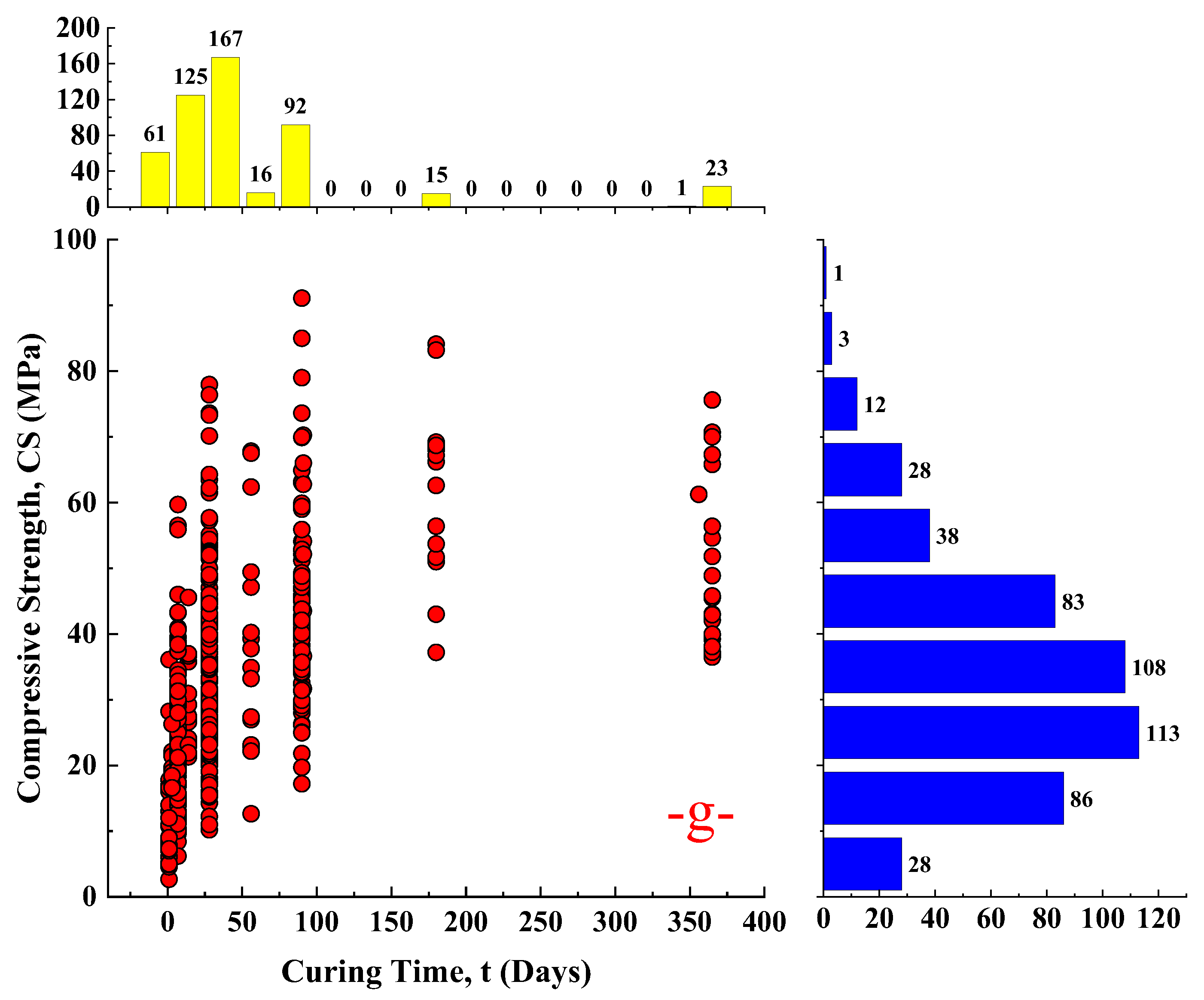
3.7. Curing Time

The median curing time in the data was 28 days, and the curing time ranged from 1 to 365 days. The statistical analysis revealed the following values for the other variables: variance of 7524 the standard deviation of 86.74, skewness, and kurtosis values of 2.69 and 6.73, respectively (Figure 2g) (Table 2).

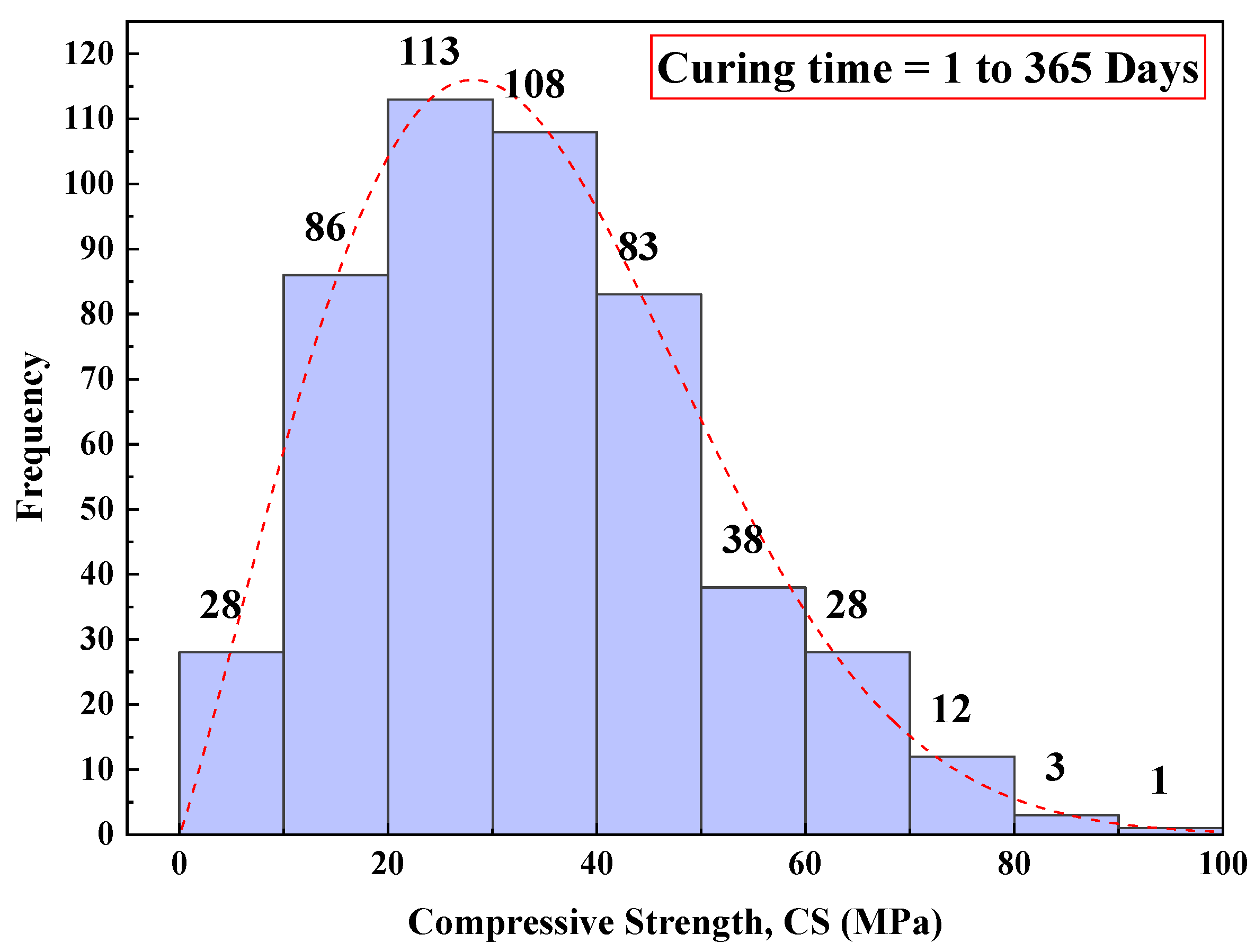
3.8. Compressive Strength

The compressive strength of SCC mix modified with FA ranged from 2.67 to 91.1 MPa, with a median of 34.9 MPa, according to the total amount of data gathered. According to the statistical analysis, the other variables had the following values: variance of 346.64, the standard deviation of 18.61, skewness of 0.48, and kurtosis of −0.38. Figure 3 displays the SCC compressive strength histogram.

4. Modeling

From the results of the analyzed data in Section 3, no direct relationship was obtained according to the correlation matrix (Figure 5). Therefore, three models were predicted to evaluate each parameter’s influence on the strength of self-compacting concrete modified with FA. All models were assessed using several standard evaluation criteria to compare all models and select the most accurate ones, such as highest R2, lower MAE, RMSI, and SI values. The models proposed in this study are used to predict the compressive strength of FA-self-compacted concrete and select the best model, which gives a better estimation of compressive strength than the measured compressive strength from the experimental data. The collected datasets were randomly split into training, testing, and validating [34]. The training dataset was used to train the LR, NLR, and MLR models and obtain the optimal weights and biases, while the testing dataset was used to confirm the fulfillment of the proposed models. The comparison among model predictions was made based on the following assessment criteria: the model should be scientifically valid, and it should give less error between the measured and predicted data, a lower RMSE, OBJ, and SI, and a higher R² value.

4.1. Nonlinear Model (LR)

This study is focused on developing a model that assesses the impact of the greatest number of parameters on the compressive strength of SCC modified with FA, as was previously mentioned. This study’s general technique for assessing compressive strength [47,48,49] is nonlinear regression.

$$\mathrm{CS}=\mathrm{a}\ast {\left(\frac{\mathrm{w}}{\mathrm{c}}\right)}^{\mathrm{b}}\ast {\left(\mathrm{C}\right)}^{\mathrm{c}}\ast {\left(\mathrm{G}\right)}^{\mathrm{d}}\ast {\left(\mathrm{S}\right)}^{\mathrm{e}}\ast {\left(\mathrm{FA}\right)}^{\mathrm{f}}\ast {\left(\mathrm{SP}\right)}^{\mathrm{g}}\ast {\left(\mathrm{t}\right)}^{\mathrm{h}}+\mathrm{i}\ast {\left(\frac{\mathrm{w}}{\mathrm{c}}\right)}^{\mathrm{j}}\ast {\left(\mathrm{C}\right)}^{\mathrm{k}}\ast {\left(\mathrm{G}\right)}^{\mathrm{l}}\ast {\left(\mathrm{S}\right)}^{\mathrm{m}}\ast {\left(\mathrm{SP}\right)}^{\mathrm{n}}\ast {\left(\mathrm{t}\right)}^{\mathrm{o}}+\mathrm{p}$$

(1)

where w/c denotes the water to cement ratio (percent), C is the cement content (kg/m³), G represents the gravel content (kg/m³), S is the sand content (kg/m³), SP is the superplasticizer content (kg/m³), FA is the fly ash content (kg/m³), t is the curing time (days), and a to p are model inputs.

4.2. Multimodel (MLR)

MLR is used when the criterion variable has more than two phases. Since it may reveal the relationship between a nominal dependent variable and two or more independent variables (Equation (2)), MLR is comparable to multiple linear regression [50].

$$\mathrm{CS}=\mathrm{a}\ast {(\frac{\mathrm{w}}{\mathrm{c}})}^{\mathrm{b}}{\left(\mathrm{C}\right)}^{\mathrm{c}}{\mathrm{G}}^{\mathrm{d}}{\mathrm{S}}^{\mathrm{e}}{\mathrm{FA}}^{\mathrm{f}}{\mathrm{SP}}^{\mathrm{g}}{\mathrm{t}}^{\mathrm{h}}$$

(2)

A limitation of Equation (2) is that it cannot be used to predict the compressive strength of SCC in the absence of FA. In this model, the FA content ought to be greater than 0 (the constraint of Equation (2) is FA content larger than 0 percent). The (a, b, c, d, e, f, g, and h) are model parameters.

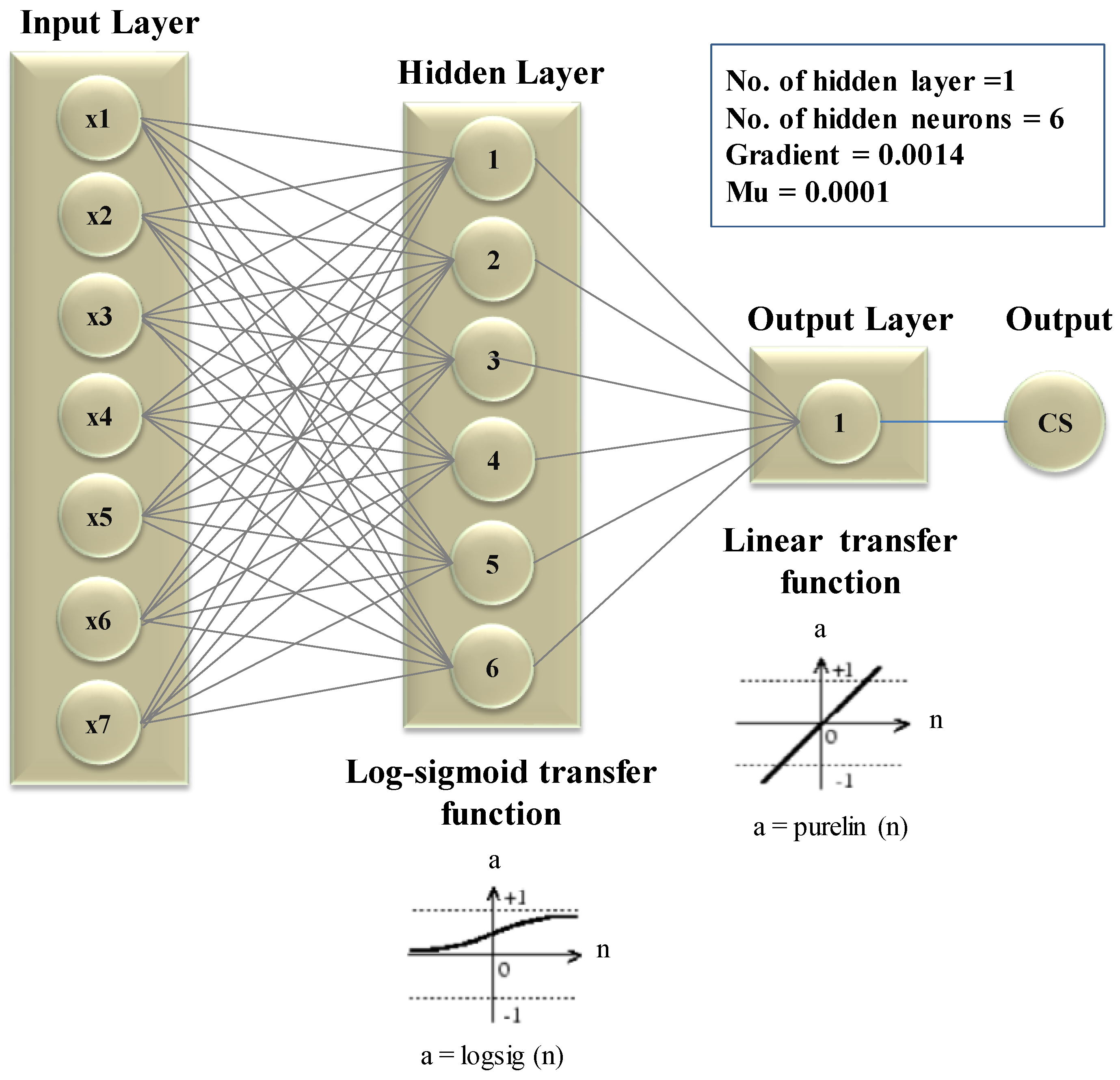
4.3. Artificial Neural Network (ANN)

A feed-forward neural network (FNN) is the opposite of an ANN [51,52,53]. Its input, output, and hidden layers are displayed in Figure 6. The input layer receives the signal to be evaluated. The input layer predicts and sort’s output. Data travel from input to output, much like an ANN’s feed-forward network. Trial and error iterations assisted in determining the model’s optimal number of hidden layers to lower error and boost R². In order to obtain the lowest RMSE, MAE, and R² values, a single hidden layer with six neural networks was selected through trial and error due to the complexity of the equation for multiple hidden layers.

$${\mathsf{\beta }}_{\mathrm{n}}={\mathrm{a}}_{\mathrm{n}}\left(\mathrm{w}/\mathrm{c}\right)+{\mathrm{b}}_{\mathrm{n}}\left(\mathrm{C}\right)+{\mathrm{c}}_{\mathrm{n}}\left(\mathrm{G}\right)+{\mathrm{d}}_{\mathrm{n}}\left(\mathrm{S}\right)+{\mathrm{e}}_{\mathrm{n}}\left(\mathrm{FA}\right)+{\mathrm{f}}_{\mathrm{n}}\left(\mathrm{SP}\right)+{\mathrm{g}}_{\mathrm{n}}\left(\mathrm{t}\right)+{\mathrm{i}}_{\mathrm{n}}$$

(3)

$$\mathrm{CS}=\frac{{\mathrm{Node}}_1}{1+{\mathrm{e}}^{-\mathsf{\beta }1}}+\frac{{\mathrm{Node}}_2}{1+{\mathrm{e}}^{-\mathsf{\beta }2}}+\cdots +\frac{{\mathrm{Node}}_{\mathrm{n}}}{1+{\mathrm{e}}^{-\mathsf{\beta }\mathrm{n}}}+\mathrm{Threshold}$$

(4)

5. Assessment Criteria for the Developed Models

The coefficient of determination (R²), root mean squared error (RMSE), mean absolute error (MAE), and scatter index (SI) was used to assess the accuracy and efficacy of the proposed models. Their equations are:

$${\mathrm{R}}^2={\left[\frac{{{\displaystyle \sum }}_{\mathrm{p}=1}^{\mathrm{p}}\left({\mathrm{t}}_{\mathrm{p}}-{\mathrm{t}}^{\prime }\right)({\mathrm{y}}_{\mathrm{p}}-{\mathrm{y}}^{\prime })}{\sqrt{\left[{{\displaystyle \sum }}_{\mathrm{p}=1}^{\mathrm{p}}{\left({\mathrm{t}}_{\mathrm{p}}-{\mathrm{t}}^{\prime }\right)}^2\right]\left[{{\displaystyle \sum }}_{\mathrm{p}=1}^{\mathrm{p}}{\left({\mathrm{y}}_{\mathrm{p}}-{\mathrm{y}}^{\prime }\right)}^2\right]}}\right]}^2,$$

(5)

$$\mathrm{RMSE} =\sqrt{\frac{{{\displaystyle \sum }}_{\mathrm{p}=1}^{\mathrm{p}}{\left({\mathrm{y}}_{\mathrm{p}}-{\mathrm{t}}_{\mathrm{p}}\right)}^2}{\mathrm{p}}},$$

(6)

$$\mathrm{MAE} =\frac{{{\displaystyle \sum }}_{\mathrm{p}=1}^{\mathrm{p}}\left|({\mathrm{y}}_{\mathrm{p}}-{\mathrm{t}}_{\mathrm{p}})\right|}{\mathrm{p}},$$

(7)

$$\mathrm{SI} =\frac{\mathrm{RMSE}}{{\mathrm{t}}^{\prime }}.$$

(8)

The predicted and measured path pattern values are denoted by y_p and t_p, respectively, and the average value of the measured and predicted values is denoted by y′ and t′. The terms tr and tst, which stand for training and testing datasets, denote the number of patterns (collected data) in each set. When evaluating any equation or model, one is the ideal value for R², but the lowest value is preferable for other parameters (MAE and RMSE), and zero is the ideal SI value. However, the SI parameter has several limitations, and when it is greater than 0.3, it indicates that the models are performing poorly.

6. Analysis and Output

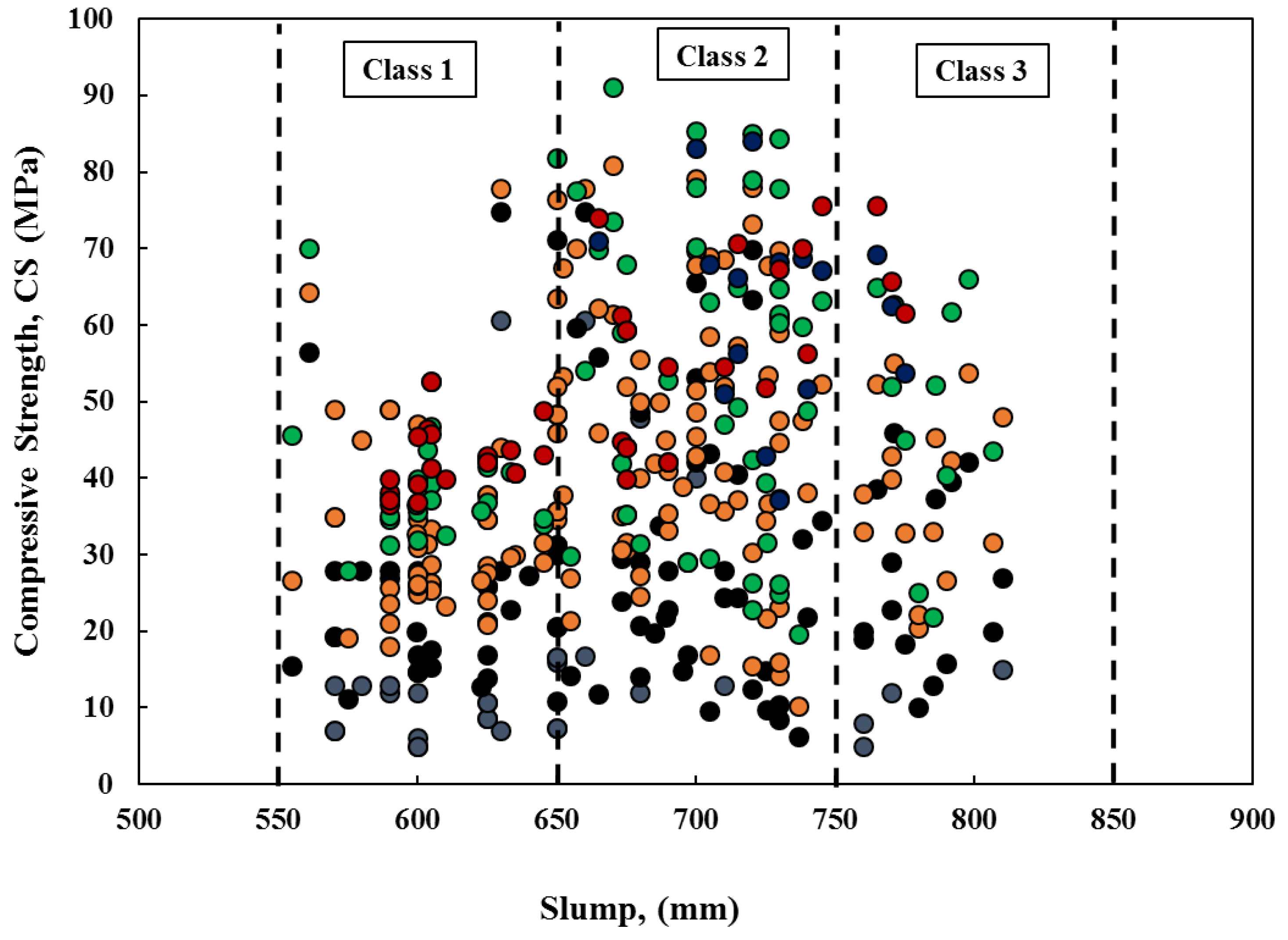
Slump Flow Diameter

The test that is most frequently used to gauge SCC flow performance is the slump flow test. During this test, the slump flow diameter of the SCC mix is measured. When using the EFNARC SCC criterion, the slump flow diameter should meet one of the classifications listed in the standard. A slump flow diameter of 550 to 650 mm is considered in slump flow class 1, 650 to 750 mm is considered in slump flow class 2, and 750 to 850 mm is considered to be in slump flow class 3 [54]. Any slump flow diameter that is both less than 550 mm and more than 850 mm cannot be classified as SCC, according to EFNARC guidelines. With a median slump flow diameter of 672 mm and minimum and maximum slump flow diameters of 550 mm and 850 mm, respectively, all of the mixes can be regarded as SCC, per 401 data (Table 1) from prior studies. Figure 7 depicts the relationship between the slump flow diameter and the CS of self-compacted concrete [4].

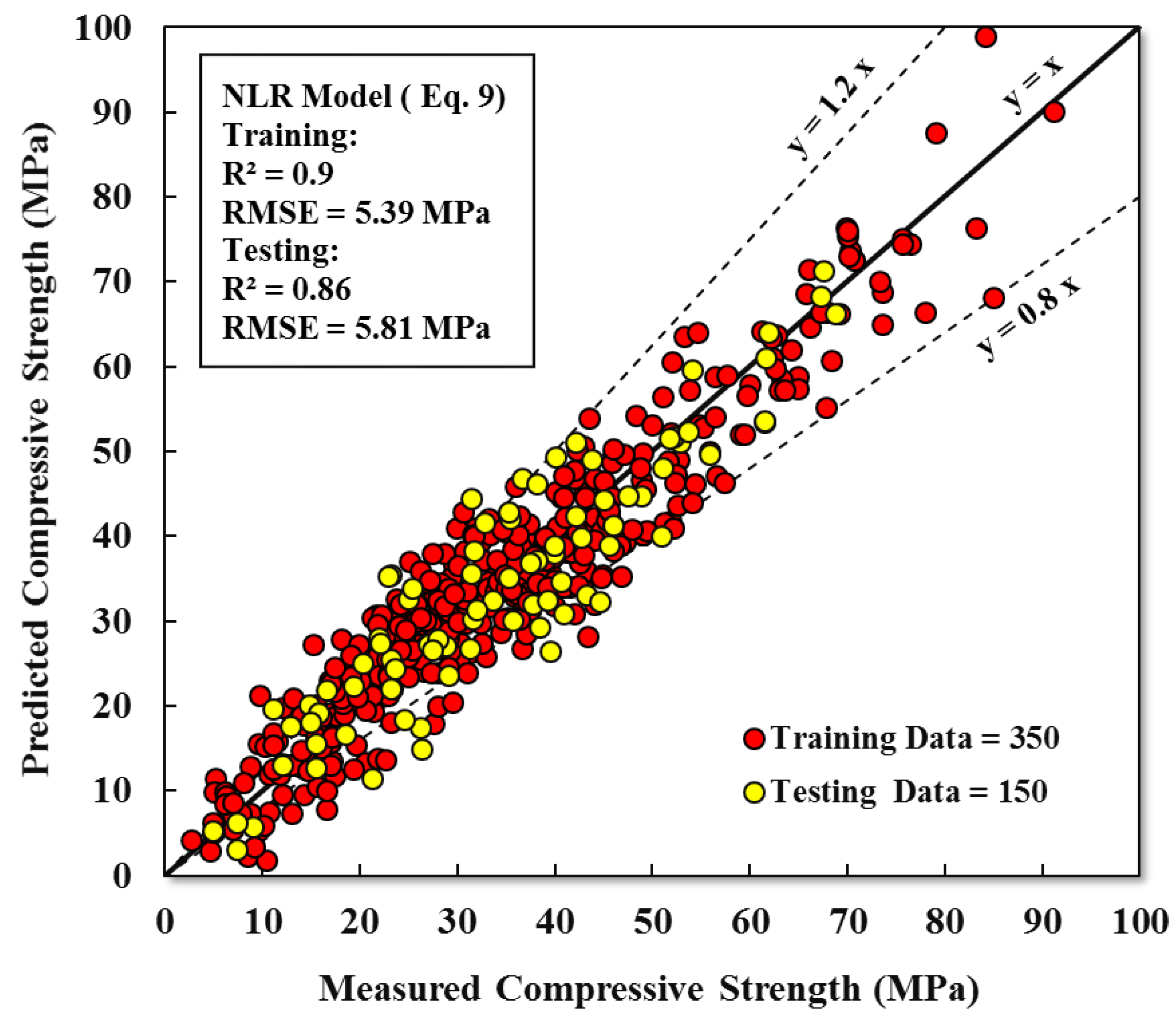
7. Nonlinear Regression Model

Figure 8 depicts the relationship between SCC’s measured and anticipated compressive strength modified with FA for training and the testing dataset. The sum of error squares and the least square method was optimized to determine the value of each parameter in the existing model. The outcome of every experiment is represented by Equation (9).

$$\mathrm{CS}=0.11{\left(\frac{\mathrm{w}}{\mathrm{b}}\right)}^{-1.196}{\left(\mathrm{C}\right)}^{0.109} {\left(\mathrm{G}\right)}^{0.628 }{\left(\mathrm{S}\right)}^{0.068} {\left(\mathrm{FA}\right)}^{-0.007} {\left(\mathrm{SP}\right)}^{0.006} {\left(\mathrm{t}\right)}^{0.104}-41.608{\left(\frac{\mathrm{w}}{\mathrm{b}}\right)}^{-1.682}{\left(\mathrm{C}\right)}^{-0.239} {\left(\mathrm{G}\right)}^{0.79} {\left(\mathrm{S}\right)}^{-0.812} {\left(\mathrm{t}\right)}^{-0.015}+0.0001.$$

(9)

According to the equation above, S has the least impact on the compressive strength of SCC modified with FA, while W has the greatest. As shown in Figure 9, the SI values for the developed model are 0.158 and 0.175 for the training and testing datasets, respectively. The values for assessment parameters such as R², RMSE, and MAE are 0.90, 5.39 MPa, and 4.35 MPa for the testing dataset.

8. Multiregression Model (MLR)

Figure 8 uses training and testing datasets for SCC modified with FA to compare the predicted compressive strength to the actual compressive strength. Following this model, the w/c ratio and sand content concentration are the most important factors affecting the compressive strength of SCC. Equation (10) can be used to represent the multi regression model with various variable parameters (Figure 10):

$$\mathrm{CS}=4.56\ast {10}^{-6}{\left(\frac{\mathrm{w}}{\mathrm{b}}\right)}^{-0.642}{\left(\mathrm{C}\right)}^{-0.487} {\left(\mathrm{G}\right)}^{0.624} {\left(\mathrm{S}\right)}^{1.146} {\left(\mathrm{FA}+0.0001\right)}^{-0.011}{\left(\mathrm{SP}\right)}^{0.008} {\left(\mathrm{t}\right)}^{0.224}.$$

(10)

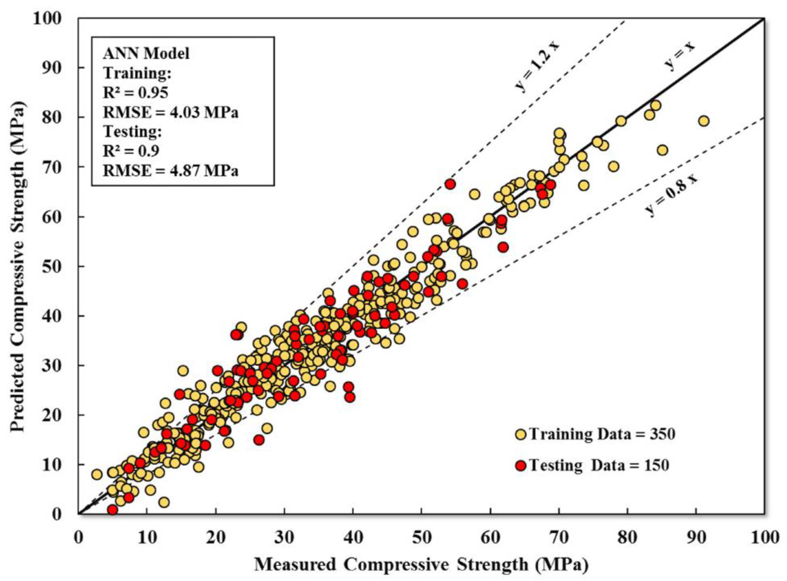
9. Artificial Neural Network (ANN)

The network was fed both training and test data to predict the compressive strength values for the appropriate input parameters (Figure 10). An ANN model was created iteratively (such as the number of hidden layer neurons, learning rate, momentum, and iteration). Nineteen neural nets were used in this study’s hidden layer system. The training period is 50,000 s, the learning rate is 0.1, and the momentum is 0.1. The quantity of epochs is a hyperparameter that controls how frequently the learning algorithm may process the training dataset. The higher the R², the lower the RMSE and, the lower the MAE is as the error is reduced, the more epochs there are. Figure 10 illustrates the basic idea of producing data using an ANN model by plotting the projected compressive strength vs. the actual value.

									w/b
−0.516	−2.554	−5.391	−4.137	−5.155	0.837	−3.108	−3.38946		C		β1
−2.950	−2.648	−2.776	−3.033	−9.037	−1.516	−0.625	−5.86885		G		β2
30.737	−11.951	−10.236	−19.384	−13.954	32.126	2.856	47.38619	×	S	=	β3
−0.507	0.047	−7.706	−5.574	−5.971	5.024	2.979	8.12332		FA		β4
61.384	−198.964	183.340	104.406	804.041	67.087	−278.128	570.3129		SP		β5
0.730	−0.299	−1.200	−0.649	−0.729	0.452	32.931	34.86496		t		β6
									1

$$\mathrm{CS}=\frac{-1.112}{1+{\mathrm{e}}^{-{\mathsf{\beta }}_1}}+\frac{0.601}{1+{\mathrm{e}}^{-{\mathsf{\beta }}_2}}-\frac{0.222}{1+{\mathrm{e}}^{-{\mathsf{\beta }}_3}}+\frac{0.529}{1+{\mathrm{e}}^{-{\mathsf{\beta }}_4}}-\frac{0.179}{1+{\mathrm{e}}^{-{\mathsf{\beta }}_5}}\frac{1.801}{1+{\mathrm{e}}^{-{\mathsf{\beta }}_6}}-2.071$$

(11)

The R², RMSE, and MAE values for this model are, respectively, 0.95, 4.03 MPa, and 3.04 MPa.

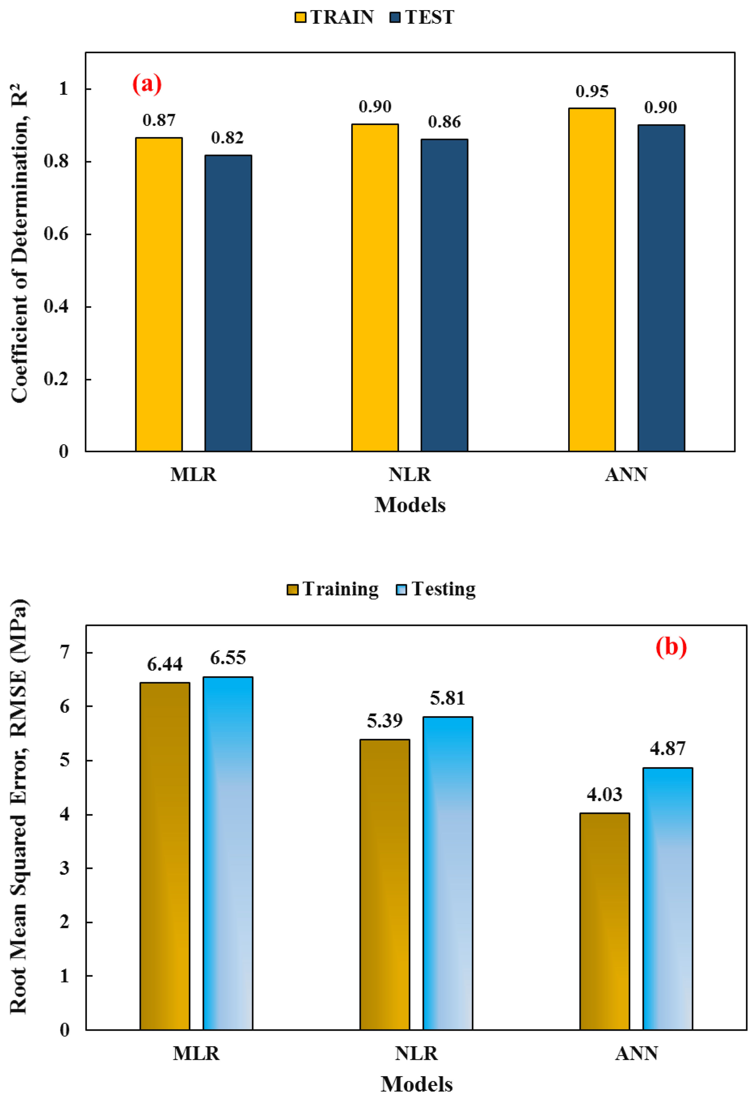
10. Comparison between Developed Models

As mentioned in earlier sections, the effectiveness of the suggested new models was evaluated using four statistical parameters (R², MAE, RMSE, and SI). Compared to the NLR and MLR models, the ANN model had the lowest RMSE and MAE values and the highest R² values. The coefficient of determination for all models using training and test sets is shown in Figure 9. Figure 9 demonstrates that the ANN model’s predicted and measured compressive strength values are much more comparable, demonstrating the ANN model’s superior performance to other models.

The SI assessment parameter values for the proposed models during the training and testing phases are shown in Figure 9. The SI values for all models and phases (training and testing), as displayed in Figure 9, were less than 0.2, indicating excellent performance for all models. Additionally, the SI values for the ANN model and the other performance parameters are lower compared to other models. The ANN model has smaller SI value values across all phases compared to the NLR model, for instance, 208 percent lower in training and 68 percent lower in testing datasets.

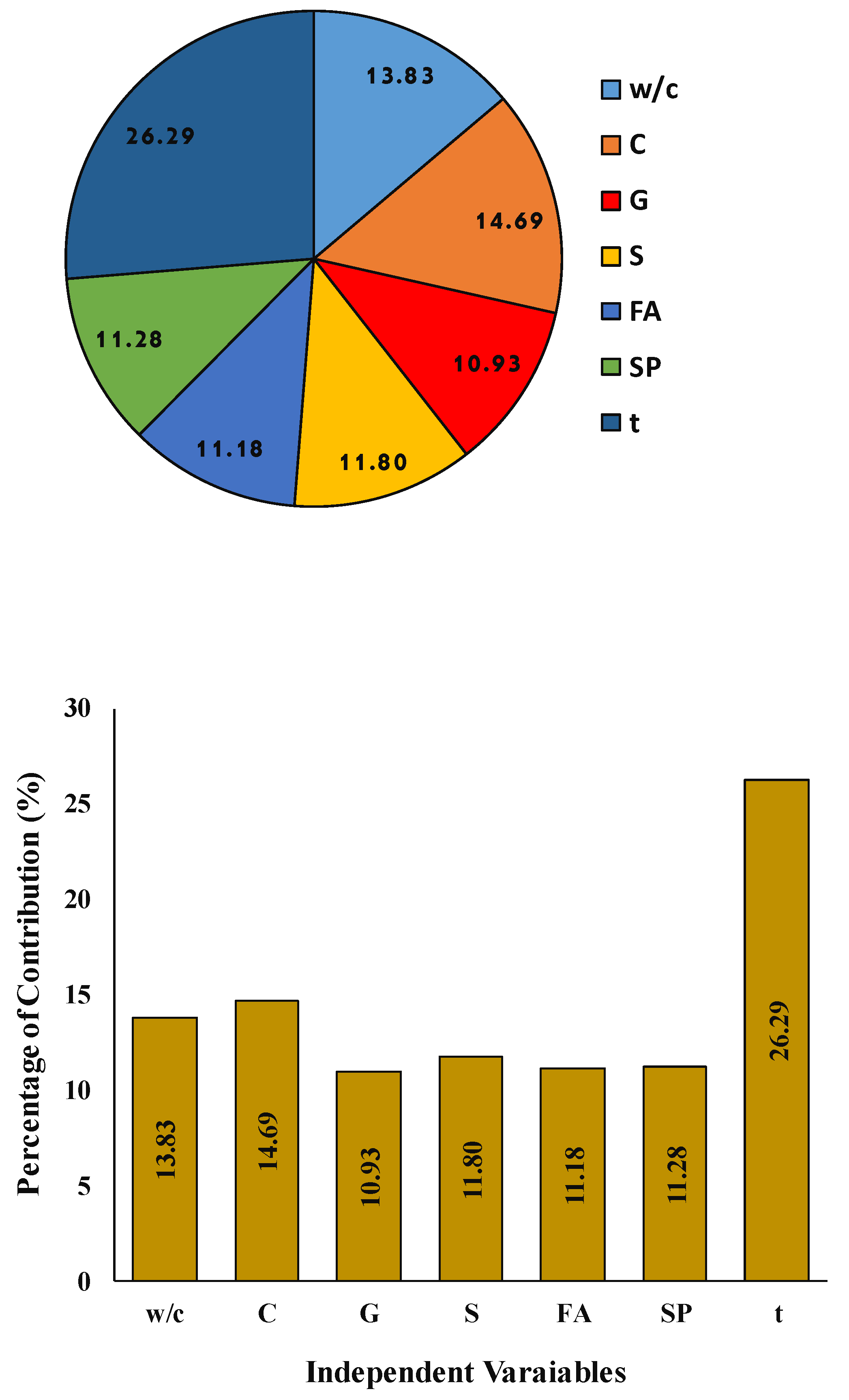
11. Sensitivity Investigation

The most important factor affecting the CS of SCC combinations was identified and evaluated using a model sensitivity test. As a quick method, the ANN model was used to examine sensitivity. Sensitivity analysis was performed, with each training dataset having only one input variable extracted. Each training dataset’s evaluation criteria, such as R2, RMSE, and MAE, were developed separately. According to the data, the curing time, cement content, and the proportion of water to cement are the factors most strongly influencing SCC compressive strength. The CS was thus greatly improved by lengthening the curing time and cement content. Figure 11 depicts the effect of mixed proportions on the CS of SCC. The capacity of models to predict the compression strength of SCC with FA for the training and test dataset was thoroughly evaluated by the following metrics: coefficient of determination (R²), root mean square error (RMSE), scatter index (SI), and mean absolute error (MAE). However, the R² value, also known as the coefficient of determination, has been observed to be the best for model assessment [4]. R² values from 0.70 to 0.80 indicate satisfactory results, values from 0.80 to 0.95 indicate good model prediction, and values above 0.95 indicate excellent prediction, while values below 0.60 indicate unsatisfactory results [4,13]. In addition, sensitivity analysis was also carried out. The results of these analyses are presented in detail in the text (Figure 12).

12. Conclusions

Based on the analysis and simulation of data from earlier studies to forecast the compressive strength of SCC for 400 different mix proportions, the following conclusions were made:

• Based on data collected from the literature, the fly ash enhanced the compressive strength of normal concrete as a partial replacement for cement. Depending on the statistical analysis, the median percentage of superplasticizers for the production of SCC was 1.33%. Furthermore, the percentage of fly ash inside all mixes ranged from 0 to 100%, with 1 to 365 days of curing and sand content ranging from 845 to 1066 kg/m³.
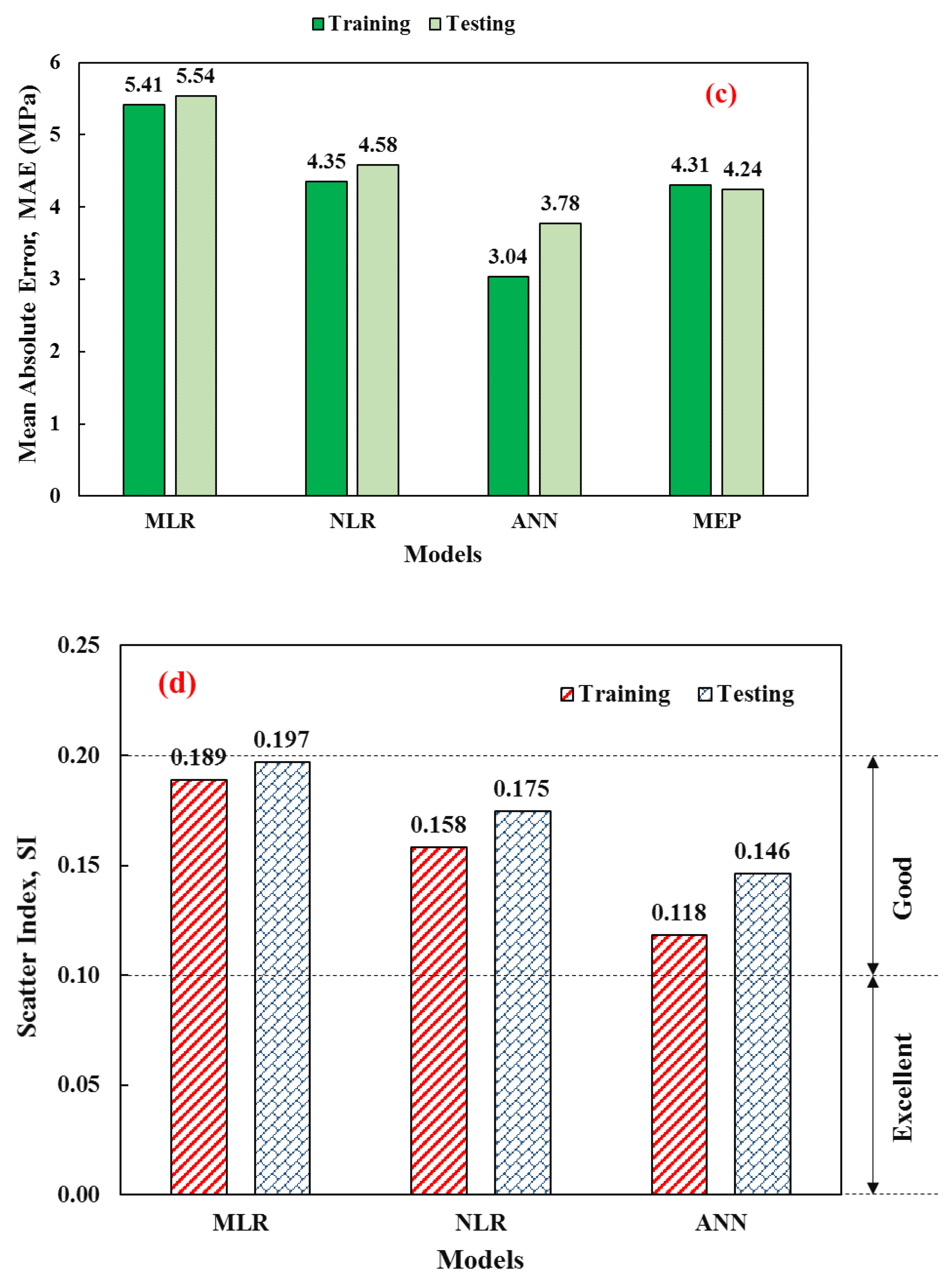
• This study developed the NLR, MLR, and ANN models to predict the compressive strength of SCC mixes. The ANN model outperformed other models in the training and testing datasets, with higher R² values, and lower RMSE, MAE, and SI values.
• The SI values for all models and phases (training and testing) were less than 0.2, indicating good performance. Furthermore, compared to the NLR model, the ANN model has smaller SI values in all phases, for example, 60% lower in training and 35% lower in the testing dataset.
• Using several evaluation criteria, including the root mean square error (RMSE), the coefficient of determination (R²), the SI, and the mean absolute error (MAE). The sequence of ANN models was the best model provided in this research based on data acquired from the literature and produced a higher R² and lower MAE and RMSE.
• The sensitivity analysis test was performed in order to check the most effective dependent variables on independent variables’ output performance. The results indicated that the most effective parameters causing the output result were curing time and fly ash content.
• The box plot for the proposed models indicated that the ANN model had better centered mean square error and standard deviation performance.
• The NLR model as a reliable mathematical model can predict the compressive strength of self-compacted concrete with a high coefficient of determination value.
• The overall findings and analysis showed that it was possible to effectively modify SCC’s strength and other properties by producing replacement SCC with cement containing 35% fly ash. However, percentages more than 35% might be detrimental to SCC’s performance.
• The sensitivity analysis showed that the curing time is the key input parameter that influences the improvement rate and forecasts the compressive strength of SCC.

References

- Satish, K.; Kumar, S.; Rai, B. Self-compacting concrete using fly ash and silica fumes as pozzolanic material. J. Eng. Technol. 2017, 6, 394–407. [Google Scholar]
- Okamura, H. Self-compacting high-performance concrete. Concr. Int. 1997, 19, 50–54. [Google Scholar]
- Sonebi, M. Medium strength self-compacting concrete containing fly ash: Modelling using factorial experimental plans. Cem. Concr. Res. 2004, 34, 1199–1208. [Google Scholar] [CrossRef]
- Faraj, R.H.; Mohammed, A.A.; Mohammed, A.; Omer, K.M.; Ahmed, H.U. Systematic multiscale models to predict the compressive strength of self-compacting concretes modified with nanosilica at different curing ages. Eng. Comput. 2021, 1–24. [Google Scholar] [CrossRef]
- Siddique, R. Properties of self-compacting concrete containing class F fly ash. Mater. Des. 2011, 32, 1501–1507. [Google Scholar] [CrossRef]
- Toporov, D. Combustion of Pulverised Coal in a Mixture of Oxygen and Recycled Flue Gas; Elsevier: Amsterdam, The Netherlands, 2014. [Google Scholar]
- Khalil, N.; Hassan, E.; Shakdofa, M.; Farahat, M. Beneficiation of the huge waste quantities of barley and rice husks as well as coal fly ashes as additives for Portland cement. J. Ind. Eng. Chem. 2014, 20, 2998–3008. [Google Scholar] [CrossRef]
- Meshram, P.; Purohit, B.K.; Sinha, M.K.; Sahu, S.K.; Pandey, B.D. Demineralization of low grade coal—A review. Renew. Sustain. Energy Rev. 2015, 41, 745–761. [Google Scholar] [CrossRef]
- Domone, P.; Hsi-Wen, C. Testing of binders for high performance concrete. Cem. Concr. Res. 1997, 27, 1141–1147. [Google Scholar] [CrossRef]
- Sunarmasto; Kristiawan, S.A. Effect of Fly Ash on Compressive Strength and Porosity of Self-Compacting Concrete. Appl. Mech. Mater. 2015, 754–755, 447–451. [Google Scholar] [CrossRef]
- Faraj, R.H.; Sherwani, A.F.H.; Jafer, L.H.; Ibrahim, D.F. Rheological behavior and fresh properties of self-compacting high strength concrete containing recycled PP particles with fly ash and silica fume blended. J. Build. Eng. 2021, 34, 101667. [Google Scholar]
- Neville, A.M.; Brooks, J.J. Concrete Technology; Longman Scientific & Technical: London, UK, 1987; pp. 242–246. [Google Scholar]
- Neville, A.M. Properties of Concrete; Longman: London, UK, 1995; Volume 4. [Google Scholar]
- Shariati, M.; Mafipour, M.S.; Ghahremani, B.; Azarhomayun, F.; Ahmadi, M.; Trung, N.T.; Shariati, A. A novel hybrid extreme learning machine–grey wolf optimizer (ELM-GWO) model to predict compressive strength of concrete with partial replacements for cement. Eng. Comput. 2020, 38, 757–779. [Google Scholar] [CrossRef]
- Silvestre, J.; de Brito, J. Review on concrete nanotechnology. Eur. J. Environ. Civ. Eng. 2016, 20, 455–485. [Google Scholar] [CrossRef]
- Karamoozian, A.; Karamoozian, M.; Ashrafi, H. Effect of Nano Particles on Self Compacting Concrete: An Experimental Study. Life Sci. J. 2013, 10, 95–101. [Google Scholar]
- Larsen, O.; Naruts, V.; Aleksandrova, O. Self-compacting concrete with recycled aggregates. Mater. Today Proc. 2019, 19, 2023–2026. [Google Scholar] [CrossRef]
- Ghasemi, M.; Mousavi, S.R. Studying the fracture parameters and size effect of steel fiber-reinforced self-compacting concrete. Constr. Build. Mater. 2019, 201, 447–460. [Google Scholar] [CrossRef]
- Dinakar, P.; Manu, S. Concrete mix design for high strength self-compacting concrete using metakaolin. Mater. Des. 2014, 60, 661–668. [Google Scholar] [CrossRef]
- Ahmadi, M.A.; Alidoust, O.; Sadrinejad, I.; Nayeri, M. Development of mechanical properties of self compacting concrete contain rice husk ash. Int. J. Comput. Inf. Syst. Sci. Eng. 2007, 1, 259–262. [Google Scholar]
- Quercia, G.; Spiesz, P.; Hüsken, G.; Brouwers, H. SCC modification by use of amorphous nano-silica. Cem. Concr. Compos. 2014, 45, 69–81. [Google Scholar] [CrossRef]
- Corinaldesi, V.; Moriconi, G. Characterization of self-compacting concretes prepared with different fibers and mineral additions. Cem. Concr. Compos. 2011, 33, 596–601. [Google Scholar] [CrossRef]
- Yu, P.; Fu, X.; Fan, M. An Artificial Neural Network Model for Flexoelectric Actuation and Control of Beams. In Proceedings of the ASME 2021 International Mechanical Engineering Congress and Exposition, Virtual Online, 1–5 November 2021; Volume 7A: Dynamics, Vibration, and Control. p. V07AT07A049. [Google Scholar]
- Min, H.; Zhang, J.; Fan, M. Size Effect of a Piezoelectric Patch on a Rectangular Plate with the Neural Network Model. Materials 2021, 14, 3240. [Google Scholar] [CrossRef]
- Jin, L.; Li, S.; Yu, J.; He, J. Robot manipulator control using neural networks: A survey. Neurocomputing 2018, 285, 23–34. [Google Scholar] [CrossRef]
- Mair, C.; Kadoda, G.; Lefley, M.; Phalp, K.; Schofield, C.; Shepperd, M.; Webster, S. An investigation of machine learning based prediction systems. J. Syst. Softw. 2000, 53, 23–29. [Google Scholar] [CrossRef]
- Milačić, L.; Jović, S.; Vujović, T.; Miljković, J. Application of artificial neural network with extreme learning machine for economic growth estimation. Phys. A Stat. Mech. Its Appl. 2017, 465, 285–288. [Google Scholar] [CrossRef]
- Jamei, M.; Mohammed, A.S.; Ahmadianfar, I.; Sabri, M.M.S.; Karbasi, M.; Hasanipanah, M. Predicting Rock Brittleness Using a Robust Evolutionary Programming Paradigm and Regression-Based Feature Selection Model. Appl. Sci. 2022, 12, 7101. [Google Scholar] [CrossRef]
- Sor, N.A.H. The effect of superplasticizer dosage on fresh properties of self-compacting lightweight concrete produced with coarse pumice aggregate. J. Garmian Univ. 2018, 5, 190–209. [Google Scholar]
- Madandoust, R.; Ranjbar, M.M.; Ghavidel, R.; Shahabi, S.F. Assessment of factors influencing mechanical properties of steel fiber reinforced self-compacting concrete. Mater. Des. 2015, 83, 284–294. [Google Scholar] [CrossRef]
- Ghafor, K.; Mahmood, W.; Qadir, W.; Mohammed, A. Effect of Particle Size Distribution of Sand on Mechanical Properties of Cement Mortar Modified with Microsilica. ACI Mater. J. 2020, 117, 47–60. [Google Scholar] [CrossRef]
- Salih, A.; Rafiq, S.; Mahmood, W.; Al-Darkazali, H.; Noaman, R.; Ghafor, K.; Qadir, W. Systemic multi-scale approaches to predict the flowability at various temperature and mechanical properties of cement paste modified with nano-calcium carbonate. Constr. Build. Mater. 2020, 262, 120777. [Google Scholar] [CrossRef]
- Salih, A.; Rafiq, S.; Mahmood, W.; Ghafor, K.; Sarwar, W. Various simulation techniques to predict the compressive strength of cement-based mortar modified with micro-sand at different water-to-cement ratios and curing ages. Arab. J. Geosci. 2021, 14, 411. [Google Scholar] [CrossRef]
- EFNARC, F. Specification and Guidelines for Self-Compacting Concrete; European Federation of Specialist Construction Chemicals and Concrete System: Farnham, UK, 2002. [Google Scholar]
- Rafiq, S.K. Modeling and statistical assessments to evaluate the effects of fly ash and silica fume on the mechanical properties of concrete at different strength ranges. J. Build. Pathol. Rehabil. 2020, 5, 441. [Google Scholar] [CrossRef]
- Arivalagan, S. Experimental Analysis of Self Compacting Concrete Incorporating Different Range of High-Volumes of Class F Fly Ash. Sch. J. Eng. Technol. 2013, 1, 104–111. [Google Scholar]
- Krishnapal, P.; Yadav, R.K.; Rajeev, C. Strength characteristics of self compacting concrete containing fly ash. Res. J. Eng. Sci. ISSN 2013, 2278, 9472. [Google Scholar]
- Abdalhmid, J.M.; Ashour, A.F.; Sheehan, T. Long-term drying shrinkage of self-compacting concrete: Experimental and analytical investigations. Constr. Build. Mater. 2019, 202, 825–837. [Google Scholar] [CrossRef]
- Bingöl, A.F.; Tohumcu, İ. Effects of different curing regimes on the compressive strength properties of self compacting concrete incorporating fly ash and silica fume. Mater. Des. 2013, 51, 12–18. [Google Scholar] [CrossRef]
- Ahmed, H.U.; Mahmood, L.J.; Muhammad, M.A.; Faraj, R.H.; Qaidi, S.M.; Sor, N.H.; Mohammed, A.S.; Mohammed, A.A. Geopolymer concrete as a cleaner construction material: An overview on materials and structural performances. Clean. Mater. 2022, 5, 100111. [Google Scholar] [CrossRef]
- Patel, R. Development of Statistical Models to Simulate and Optimize Self-Consolidating Concrete Mixes Incorporating High Volumes of Fly Ash. Master’s Thesis, Ryerson University, Toronto, ON, Canada, 2004; p. 1802. [Google Scholar]
- Şahmaran, M.; Yaman, İ.Ö.; Tokyay, M. Transport and mechanical properties of self consolidating concrete with high volume fly ash. Cem. Concr. Compos. 2009, 31, 99–106. [Google Scholar] [CrossRef]
- Güneyisi, E.; Gesoğlu, M.; Özbay, E. Strength and drying shrinkage properties of self-compacting concretes incor-porating multi-system blended mineral admixtures. Constr. Build. Mater. 2010, 24, 1878–1887. [Google Scholar] [CrossRef]
- Siddique, R.; Aggarwal, P.; Aggarwal, Y. Influence of water/powder ratio on strength properties of self-compacting concrete containing coal fly ash and bottom ash. Constr. Build. Mater. 2012, 29, 73–81. [Google Scholar] [CrossRef]
- Dhiyaneshwaran, S.; Ramanathan, P.; Baskar, I.; Venkatasubramani, R. Study on durability characteristics of self-compacting concrete with fly ash. Jordan J. Civ. Eng. 2013, 7, 342–353. [Google Scholar]
- Bouzoubaâ, N.; Lachemi, M. Self-compacting concrete incorporating high volumes of class F fly ash: Preliminary results. Cem. Concr. Res. 2001, 31, 413–420. [Google Scholar] [CrossRef]
- Nikbin, I.; Beygi, M.; Kazemi, M.; Amiri, J.V.; Rahmani, E.; Rabbanifar, S.; Eslami, M. A comprehensive investigation into the effect of aging and coarse aggregate size and volume on mechanical properties of self-compacting concrete. Mater. Des. 2014, 59, 199–210. [Google Scholar] [CrossRef]
- Wang, J.; Mohammed, A.S.; Macioszek, E.; Ali, M.; Ulrikh, D.V.; Fang, Q. A Novel Combination of PCA and Machine Learning Techniques to Select the Most Important Factors for Predicting Tunnel Construction Performance. Buildings 2022, 12, 919. [Google Scholar] [CrossRef]
- Mohammed, A.; Rafiq, S.; Sihag, P.; Kurda, R.; Mahmood, W. Soft computing techniques: Systematic multiscale models to predict the compressive strength of HVFA concrete based on mix proportions and curing times. J. Build. Eng. 2020, 33, 101851. [Google Scholar] [CrossRef]
- Salih, A.; Rafiq, S.; Sihag, P.; Ghafor, K.; Mahmood, W.; Sarwar, W. Systematic multiscale models to predict the effect of high-volume fly ash on the maximum compression stress of cement-based mortar at various water/cement ratios and curing times. Measurement 2020, 171, 108819. [Google Scholar] [CrossRef]
- Mohammed, A.; Rafiq, S.; Mahmood, W.; Al-Darkazalir, H.; Noaman, R.; Qadir, W.; Ghafor, K. Artificial Neural Network and NLR techniques to predict the rheological properties and compression strength of cement past modified with nanoclay. Ain Shams Eng. J. 2020, 12, 1313–1328. [Google Scholar] [CrossRef]
- Mohammed, A.; Mahmood, W. Statistical Variations and New Correlation Models to Predict the Mechanical Behavior and Ultimate Shear Strength of Gypsum Rock. Open Eng. 2018, 8, 213–226. [Google Scholar] [CrossRef]
- Mahmood, W.; Mohammed, A. Hydraulic Conductivity, Grain Size Distribution (GSD) and Cement Injectability Limits Predicted of Sandy Soils Using Vipulanandan Models. Geotech. Geol. Eng. 2020, 38, 2139–2158. [Google Scholar] [CrossRef]
- Akeed, M.H.; Qaidi, S.; Faraj, R.H.; Mohammed, A.S.; Emad, W.; Tayeh, B.A.; Azevedo, A.R. Ultra-high-performance fiber-reinforced concrete. Part II: Hydration and microstructure. Case Stud. Constr. Mater. 2022, 17, e01289. [Google Scholar] [CrossRef]