Complete Blood Cell Detection and Counting Based on Deep Neural Networks

Abstract

Complete blood cell (CBC) counting has played a vital role in general medical examination. Common approaches, such as traditional manual counting and automated analyzers, were heavily influenced by the operation of medical professionals. In recent years, computer-aided object detection using deep learning algorithms has been successfully applied in many different visual tasks. In this paper, we propose a deep neural network-based architecture to accurately detect and count blood cells on blood smear images. A public BCCD (Blood Cell Count and Detection) dataset is used for the performance evaluation of our architecture. It is not uncommon that blood smear images are in low resolution, and blood cells on them are blurry and overlapping. The original images were preprocessed, including image augmentation, enlargement, sharpening, and blurring. With different settings in the proposed architecture, five models are constructed herein. We compare their performance on red blood cells (RBC), white blood cells (WBC), and platelet detection and deeply investigate the factors related to their performance. The experiment results show that our models can recognize blood cells accurately when blood cells are not heavily overlapping.

1. Introduction

For an adult, there are about five liters of blood in the body, and blood cells account for nearly 45% of blood tissue by volume. Three blood cell types are red blood cells (RBC), white blood cells (WBC, including basophil, lymphocyte, neutrophil, monocyte, and eosinophil) and platelets. Red blood cells are the main medium carrying oxygen, white blood cells are a part of the immunity system resisting diseases, and platelets have coagulation function, which can recover wounds with scabs. Both physiological and pathologic changes affect the composition of blood clinically. Thus, blood tests have become a direct channel to detect one’s health status or diagnose diseases. Complete blood cell (CBC) counting is one of the classical blood tests, which identifies and counts basic blood cells to examine, follow and manage the variation in blood [1].

CBC counting is often performed by flow cytometers or medical professionals to obtain reliable test results. However, manual operation is time-consuming, tedious, and fallible. Scientists began exploiting automated analyzers in the early 20th century. With the development of computation capabilities, many researchers adopt image processing techniques and statistical or deep learning models to elevate CBC counting on blood smear images. However, the blood smear images for CBC counting are usually low resolution and blurry, making it hard to accurately identify blood cells. Furthermore, blood cells are sometimes heavily overlapping. We will further survey these studies in Section 2.

Convolutional Neural Networks (CNNs) have been applied successfully in several visual recognition tasks [2]. Due to their outstanding abilities of learning and extracting features, CNNs have become a prevalent approach in dealing with medical image analysis [3]. Well-trained CNNs can capture more useful information and better detect and classify objects on input images than traditional image processing methods. In addition, CNNs can be easily integrated into information systems and have been widely adopted in big data information processing [4].

In this paper, we propose a novel CNN-based deep learning architecture to detect and classify blood cells on blood smear images and simultaneously realize accurate CBC counting. Five models are constructed herein with different settings. The experiments are carried out on a public blood smear image dataset. In the end, we compare and discuss the results of the proposed models under different conditions.

In this paper, we introduce the research background, motivation, and objective in Section 1. We survey related works in the literature in Section 2. We then describe the proposed architecture in Section 3. We show and discuss the experimental results in Section 4. Finally, we draw conclusions in Section 5.

2. Related Works

Traditionally, CBC counting was accomplished by manually manipulating the hemocytometer, flow cytometry, and chemical compounds [5]. The professional knowledge of clinical laboratory analysts influenced the outcomes of cases [6,7]. The entire procedure was highly time-consuming and error-prone. Later, with well-developed computational skills and counting methods in image processing, mainstream research explored handcrafted features and used statistical models to detect and classify blood cells. In recent years, automated CBC counting is usually accomplished with the use of image processing and machine learning [5].

2.1. Early History of Complete Blood Cell Counting

The observation of blood cells emerged when van Leeuwenhoek inspected his blood in 1675 [8]. Since the earliest time, scientists have carried on with microscopic investigations. They observed and analyzed blood cells while continuing to improve microscope technology during the 18th and 19th centuries. The first blood cell counting based on a microscope was accomplished by Vierordt in 1852, and the hemocytometer was launched in 1874, leading to more accurate results [8,9]. Research on automated blood cell counting started in the early 20th century. One RBC counting method published in 1928 used photometry to estimate the blood volume but failed in accurately assessing abnormal cells [10]. Other approaches integrated photoelectric detectors and microscopes also generated discouraging counting results over the next twenty years [9]. In the 1950s, the Coulter counter was introduced, which passed cells through an aperture to do the counting and estimate the sizes of RBC by using the conductivity of the blood as the reference [11]. The Coulter counter was modified and applied to RBC and WBC counting; the Technicon SMA 4A−7A could simultaneously examine multiple cells [12]. Automated platelet counts with Technicon Hemalog-8 were presented in 1970 and integrated into Coulter’s S Plus series analyzers in 1980 [9]. The examination of blood samples mostly employed laboratory analysts. They operate automated analyzers to collect information, annotate blood smear images, and recheck them when ambiguous cases are encountered.

2.2. Traditional Image Processing-Based Methods

Madhloom et al. proposed an automated WBC detection and classification process that used a combination of several image processing techniques to separate the nucleus from target cells in 2010 [13]. Firstly, they converted images into grayscale and removed the darkest part as the nucleus from the WBCs. Then they utilized automatic contrast stretching, histogram equalization, and image arithmetic to localize the nucleus and applied an automatic global threshold to carry out the segmentation. The nucleuses would be identified with types of leukocytes after passing through a minimum filter and automatic threshold. The proposed model finally achieved accuracy between 85 and 98%.

Another piece of research on automatic WBC recognition was proposed by Rezatofighi et al. in 2011 [14]. They exploited the Gram–Schmidt method to segment nuclei in the beginning and then distinguished basophils. A Snake algorithm was used to divide the cytoplasm. The color, morphology, and texture features were extracted and fed into two classifiers: SVM (Support Vector Machine) and ANN (Artificial Neural Network). It obtained a 93% segmentation result and 90% and 96% classification accuracies, respectively.

In addition, Acharya and Kumar proposed an imaging processing technique for RBC counting and identification in 2018 [15]. They applied the K-medoids algorithm and Granulometric analysis to separate the RBCs from the abstracted WBCs and then counted the RBCs by labeling the algorithm and circular Hough transform. A comparison was taken, and the results demonstrated that the circular Hough transform outperformed in the counting and the labeling algorithm and was successful in recognizing whether or not the RBC was normal.

For platelet counting, Kaur et al. proposed an automatic platelet counter in 2016 that employed circular Hough transform to microscopic blood images [16]. They utilized the size and shape features of platelets and achieved an accuracy of 96%. Moreover, Cruz et al. proposed an image analysis system able to segment and carry out CBC counting in 2017 [17]. Microscopic blood images would be processed by HSV thresholding, connected component labeling, and statistical analysis. The results showed that the proposed system had over 90% accuracy.

2.3. Machine Learning-Based Methods

With the rapid improvement of deep learning algorithms and computational resources, adopting deep learning for medical image analysis has become an effective and efficient approach to abstract information [18]. Various related studies implemented machine learning techniques in medical research, such as computer-aided diagnosis, medical image disease detection, and image-guided therapy [19,20]. CNNs, with strong capabilities for learning and extracting features, have been widely used in several medical fields and achieved outstanding performances making CNNs also popular in the blood cell counting and identification domains.

In 2013, Habibzadeh et al. proposed a subcomponent system that classified WBCs into five different types in low-resolution images [1]. The system employed two kinds of SVM and one CNN as classifiers, and the latter gained the best results. Su et al. proposed an ANN-based WBC classification system in 2014 [21]. They segmented WBCs, extracted the effective features, and fed the features into three kinds of ANNs to recognize the category of WBCs. The obtained a high recognition rate, which could be 99.11% correct. Similarly, Nazlibilek et al. proposed a system for automatically counting and classifying WBCs in 2014 [22]. They segmented the blood cells into sub-images and fed them into an ANN classifier. Combined with PCA (Principal Component Analysis), the ANN classifier’s success rate reached 95%.

Habibzadeh et al. later proposed a WBC classification system that used pre-trained models of ResNet and Inception [23] in 2018. The images were augmented, preprocessed by color distortion, and fed into ImageNet pre-trained ResNet and Inception networks to abstract useful features for recognition. ResNet V1 50 gained the best detection rate with an average of 100%, while ResNet V1 152 and ResNet 101 achieved 99.84% and 99.46%, respectively. Çelebi and Çöteli extended the range of identification, and the proposed system simultaneously classified RBCs and WBCs by ANN [24]. They fed segmented images into CNN-based ANN and used the IoU (Intersection over Union) threshold to examine the overlaps and count each type of blood cell.

2.4. Convolutional Neural Network

The origin of convolutional neural networks (CNN) can be dated back to the early 1960s. Hubel and Wiesel observed the activity of the visual cortex cells of cats and proposed the “receptive field” concept [25]. Fukushima and Miyake raised the idea of “neocognition” in 1982 [26], which could be considered the opening of CNN research. The first CNN structure proposed by LeCun et al. in 1989 was employed in handwritten zip code recognition and was later used as the foundation of image classification [27]. The layers in LeNet-5 can be partitioned into convolutional, pooling, and fully-connected layers. The convolutional layers are in charge of learning and abstracting features, the pooling layers reduce the resolution of feature maps to attain shift-invariance, and fully-connected layers aim to perform high-level reasoning [28].

However, a shortage of computing resources and an improper training algorithm caused the development of CNNs to stagnate for nearly 20 years. At that time, CNN was mainly applied to handwritten digit recognition tasks [26,29]. When facing complicated problems, handcrafted feature extractions and statistical methods became the primary solutions. Until the 2000s, plentiful efforts had been taken to overcome the storage of computing resources, and the concept of deep learning algorithms was also introduced [4]. Breakthroughs among various fields successfully brought CNNs back again. AlexNet [30], which outperformed in the ImageNet competition in 2012, caused CNNs to become a sensation, attracting attention in many ways. In 2014, Visual Geometry Group (VGG) proposed the VGG model, which achieved excellent success in the ImageNet competition. VGG-16 and VGG-19 have been two of the commonly used models [31]. In 2015, the Inception model was proposed to improve the utilization of computing resources [32]. In 2016, ResNet was proposed to realize the training of deep ANNs [33].

With the significant improvement of computation hardware and training algorithms, CNNs have been widely exploited in multiple domains, such as handwriting recognition, face recognition, speech recognition, image classification, object detection, and natural language processing [34]. As well, ANN-based approaches have been found to be suitable for big data analysis [4,35].

2.5. Summary

In short, CBC counting-related research can fall into three types: automated analyzer, image processing-based methods, and machine learning-based methods. An automated analyzer, which substitutes chemical manipulations and measurement, is currently the most general method, although it requires lots of time and manpower. With the development of hardware and algorithms, computer-aided methods emerged in relevant studies. Traditional image processing-based methods used various image processing techniques to extract handcrafted features and statistical classifiers for blood cell detection and recognition and achieved outstanding scores. On the other hand, machine learning-based methods built deep structures to capture more non-intuitive but useful features to better carry out CBC counting.

3. Materials and Methods

In this paper, we propose a new CNN-based deep learning architecture to detect and identify target cells in blood smear images. In Section 3.1, we describe the proposed architecture, including the generation of feature maps from input blood smear images and the detection and classification of blood cells. In Section 3.2, we enumerate the three measures: Intersection of Union (IoU), Distance-IoU (DIoU), and confusion matrix, used in this paper to evaluate the performance of our models.

3.1. Proposed Architecture

Figure 1 shows the proposed architecture.

Figure 1. The proposed architecture.

The blood smear images are first preprocessed by four stages: image augmentation, enlargement, sharpening, and blurring.

CNN, which was devoted to extracting and generating fundamental feature maps, served as the backbone of the model. In this paper, VGG-16 [31] was adopted. We then added the Region Proposal Network (RPN) introduced in Faster R-CNN [36,37,38,39,40,41] to hypothesize blood cell locations. In the RoI (Region of Interest) Pooling layer, the information from the feature maps and RPN are combined to generate potential feature vectors. The following classifier uses these feature vectors to predict the coordinates and categories of the detected blood cells.

To improve the performance of small detection, we adopted the feature fusion method [42,43] to yield better feature maps. In addition, we leveraged the Convolutional Block Attention Module (CBAM) [44] for adaptive feature refinement.

VGG-16 [31] can be considered to be a composition of five blocks with a total of 13 convolutional layers, 5 pooling layers, and 3 fully-connected layers, as shown in the upper part of Figure 2. In the convolutional layers, VGG-16 employs 3 × 3 filters to generate feature maps with different resolutions. The pooling layer performs max-pooling by a 2 × 2 window to reduce the resolution of the feature maps. The last fully-connected layer is a softmax layer in charge of classification. VGG-16 has shown its powerful capability in many visual recognition applications [34].

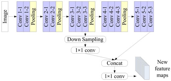
Figure 2. Feature fusion in the proposed architecture.

When an image is processed in VGG-16, the feature maps generated by the convolution layers will be reduced by max-pooling layers. The last feature maps might have insufficient information for the detection of very small objects, such as platelets. However, the feature maps generated in the middle layers still have abundant information. We adopted the feature fusion method to yield additional feature maps [42,43]. Feature fusion includes three kinds of approaches: feature ranking, feature extraction, and feature combination. Here feature combination was adopted, and the process is illustrated in Figure 2. The feature maps generated by convolution layers Conv 3-3 and Conv 5-3 were combined to provide information in higher resolution.

We further adopted the Convolutional Block Attention Module (CBAM) [44] to emphasize the meaningful features. CBAM learns channel attention and spatial attention separately. It generates channel attention maps by exploiting the inter-channel relationship between the features and then generates spatial attention maps by utilizing the channel attention maps. Channel attention focuses on what is meaningful, given the input image. Spatial attention focuses on the location of informative parts, which is complementary to channel attention.

We then adopted the architecture of Faster R-CNN [41] for blood cell detection, classification, and counting.

In 2014, Girshick et al. proposed Region-Based CNN (R-CNN) [36] for object detection. It associated CNNs with domain-specific fine-tuning. R-CNN consists of three modules: region proposals, feature extraction, and object category classifiers. Later, Fast R-CNN [39] was proposed to speed up the computation of detection networks. It generated region proposals by selective search. RoI (Region of interest) Pooling layer extracted a set of fixed-size feature maps for projected region proposals.

In 2015, Faster R-CNN was proposed; it introduced a Region Proposal Network (RPN), sharing feature maps with the CNN to yield region proposals [41]. In the RPN layer, it slid a window over the feature map to generate region proposals, also known as anchor boxes, and the corresponding lower-dimensional features. Each feature was fed into two sibling fully-connected layers in charge of regression and classification. The box-classification layer determines whether the candidate was positive (object) or negative (background), and the box-regression layer calculates the deviation of the coordinates between the ground truth and the candidate. The RoI Pooling layer combines the information of the feature maps and region proposals (or anchors) to generate fixed-size feature vectors. The following classifier used these feature vectors to predict the categories and coordinates of the detected objects.

3.2. Evaluation Measures

We used three measures: Intersection of Union (IoU), Distance-IoU (DIoU), and confusion matrix, for the bounding box and classifier evaluation.

IoU is a classical and popular measure to evaluate the similarity in object detection [45]. It calculates the ratio of intersection to union with the predicted box and ground truth box. The formula of IoU is shown in Equation (1).

$$\mathrm{IoU}=\frac{\mathrm{Ground} \mathrm{Truth} \mathrm{Bounding} \mathrm{Box} {\displaystyle \cap } \mathrm{Predicted} \mathrm{Bounding} \mathrm{Box}}{\mathrm{Ground} \mathrm{Truth} \mathrm{Bounding} \mathrm{Box} {\displaystyle \cup } \mathrm{Predicted} \mathrm{Bounding} \mathrm{Box}}$$

(1)

Figure 3 shows the intersection and union of two overlapping boxes. We assumed that Box A is for the predicted box and Box B is for the ground truth box. The red area is the intersection, and the green area is the union. The IoU of Boxes A and B was calculated by dividing the red area by the green area.

Figure 3. Intersection and Union of two overlapping boxes A and B.

In addition, we measured the Distance-IoU (DIoU) [46] of the predicted box and ground truth box. The computation of DIoU is shown by Equation (2), where d is the Euclidean distance between the central points of the two overlapping boxes, and c is the diagonal length of the smallest rectangle covering the two boxes, as shown in Figure 4.

$$\mathrm{DIoU}=\mathrm{IoU}-\frac{d^2}{c^2}$$

(2)

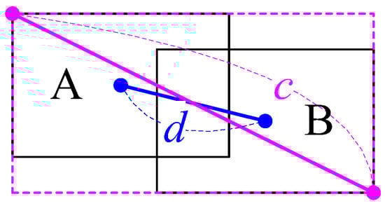
Figure 4. Distance-IoU (DIoU) calculation of two overlapping boxes.

A confusion matrix is a common measurement for the performance of a classifier in machine learning and statistics. The precision, recall, and F1 score are calculated by Equations (3)–(5).

$$\mathrm{Precision}=\frac{\mathrm{TP}}{\left(\mathrm{TP}+\mathrm{FP}\right)}$$

(3)

$$\mathrm{Recall}=\frac{\mathrm{TP}}{\left(\mathrm{TP}+\mathrm{FN}\right)}$$

(4)

$$\mathrm{F}1 \mathrm{score}=\frac{2\times \mathrm{Precision}\times \mathrm{Recall}}{\mathrm{Precision}+\mathrm{Recall}}$$

(5)

For a binary classification, TP, FN, FP, and TN refer to the following:

• True Positive (TP): both the actual and predicted classes are positive.
• False Negative (FN): a positive sample is predicted as a negative.
• False Positive (FP): a negative sample is predicted as a positive.
• True Negative (TN): both the actual and predicted classes are negative.

In this research, when a predicted bounding box and a ground truth bounding box overlay, their IoU and DIoU are higher than the specified thresholds, and they have the same category (RBC, WBC, platelets, and background); they are considered to be TP; FN, FP, and TN can be similarly defined.

4. Experiments and Results

4.1. Dataset Description

The Blood Cell Count and Detection (BCCD) dataset [47] is used in this research. It is a public dataset of annotated blood smear images for blood cell detection. It consists of 364 blood smear images with 640 × 480 pixels and an annotation file for details on the image. Each image involves arbitrary numbers of RBCs, WBCs, and platelets. The annotation file contains the information related to annotated blood cells, e.g., the coordinates of bounding boxes and categories. Figure 5 shows one of the blood smear images in the dataset with bounding boxes and labeled blood cells.

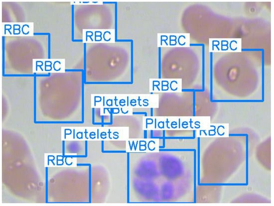
Figure 5. Original image with ground truth bounding boxes and labels.

The dataset was randomly divided into two subsets: 80% of the images were for training, and 20% of the images were for validation. Table 1 shows the numbers of three kinds of blood cells for training and validation, respectively.

Table 1. BCCD dataset.

	Training (80%)	Validation (20%)
Red Blood Cell (RBC)	3310	843
White Blood Cell (WBC)	297	75
Platelets	301	60

4.2. Data Preprocessing

The blood smear images were first preprocessed by four stages: image augmentation, enlarging, sharpening, and blurring.

To increase the number and diversity of the images, we not only applied horizontal flipping, vertical flipping, and rotation to the original images but also converted them from RGB color space into grayscale. Since it is difficult to detect small objects, such as platelets, we also used bicubic interpolation [48] to enlarge the images.

We then utilized the idea of unsharp masking to sharpen the blurry images. The procedure of unsharp masking can be divided into three phases: blur the original image, acquire the mask by deducting the blurred image from the original, and add a weighted portion of the mask back to the original [49]. In this paper, we computed the mask of an image by applying a 3 × 3 OpenCV built-in Laplacian filter and then removed a weighted portion of the mask with a parameter k from the image, shown as Equation (6).

$$f_{sharpen}\left(x,y\right)=f_{original}\left(x,y\right)-k\times f_{mask}\left(x,y\right)$$

(6)

We then blurred the images with a 3 × 3 Gaussian kernel to make them smoother.

4.3. Model Setting

We constructed five models with different settings for preprocessing. Some used enlarged images, and others used sharpened images. Some used RGB images only, while others used both RGB and grayscale images.

We then preset the parameters of RPN in the five models for blood cell detection on the images of the dataset. It is crucial to decide the scales and aspect ratios of the anchors in RPN for target-object detection. We exploited the coordinates of the bounding boxes in the annotation file. Table 2 displays the size information in the pixels of three types of blood cells.

Table 2. Blood cell size information in pixels.

	Red Blood Cell			White Blood Cell			Platelets
	Min	Mean	Max	Min	Mean	Max	Min	Mean	Max
x-axis	42	104	168	31	194	338	19	42	167
y-axis	39	100	166	27	174	286	23	40	135

We select 42, 86, and 170 pixels as anchor scales for RPN to detect objects. As well, we employ 1:1, 1/$\sqrt{2}$:$\sqrt{2}$, and $\sqrt{2}$:1/$\sqrt{2}$ as anchor aspect ratios. As a result, anchors in nine different sizes are used in RPN. Anchor scales have to be adjusted accordingly for models using enlarged images.

Table 3 shows the settings of the five proposed models. Models 1, 2, and 3 differ in the size of the input images. In models 2 and 3, the input images are enlarged by 1.25 and 1.5 times, respectively. Together, they examine the impact of enlarging the input images. In model 4, the input images are not sharpened in the preprocessing step. Models 1 and 4 examine the effect of image enhancement by sharpening. Model 5 uses the input images in the RGB color space only. Models 1 and 5 investigate the potential of grayscale blood smear images.

Table 3. Model settings.

	Model 1	Model 2	Model 3	Model 4	Model 5
Input Size	480 × 640	600 × 800	720 × 960	480 × 640	480 × 640
Enlarge	No	Yes	Yes	No	No
Anchor Boxes Size	[42, 86, 170]	[53, 107, 213]	[64, 128, 256]	[42, 86, 170]	[42, 86, 170]
Sharpen	Yes	Yes	Yes	No	Yes
Images Color	Grayscale or RGB				RGB

4.4. Experiment Results

Table 4 and Table 5 show the experiment results in the validation data of all of the models under a confidence score of 0.9 and 0.8, respectively. We note that the recall of blood cell detection also refers to the ratio of the predicted to ground truth boxes. For accurate blood cell counting, we prefer models with higher recalls. Models 1, 2, and 3, trained with preprocessed images in both grayscale and RGB color spaces, are much more powerful than the others. For the WBC recognition task, Model 1 is advantageous. For RBC recognition tasks, Model 3, trained with enlarged (1.5×) images, achieves a prominent recall and F1 score. Model 5, using only RGB images, achieves the highest precision; however, it scores worst in recall. For the platelet recognition task, Model 2, trained with enlarged (1.25×) images, achieves the best F1 scores.

Table 4. Results of the validation data of all models when confidence score is 0.9.

Type	Red Blood Cell			White Blood Cell			Platelets
Index *	P	R	F1	P	R	F1	P	R	F1
Model 1	0.737	0.744	0.741	0.761	0.95	0.845	0.498	0.412	0.451
Model 2	0.794	0.673	0.729	0.521	0.614	0.564	0.529	0.492	0.51
Model 3	0.747	0.823	0.783	0.214	0.2	0.209	0.382	0.288	0.329
Model 4	0.731	0.762	0.747	0.704	0.886	0.784	0.381	0.431	0.405
Model 5	0.808	0.517	0.631	0.487	0.936	0.641	0.114	0.067	0.085

* P, R, and F1 refer to precision, recall, and F1-score, respectively.

Table 5. Results of the validation data of all models when confidence score is 0.8.

Type	Red Blood Cell			White Blood Cell			Platelets
Index *	P	R	F1	P	R	F1	P	R	F1
Model 1	0.693	0.799	0.742	0.691	0.964	0.805	0.508	0.53	0.519
Model 2	0.761	0.748	0.755	0.536	0.7	0.607	0.47	0.67	0.553
Model 3	0.701	0.867	0.775	0.279	0.271	0.275	0.453	0.576	0.507
Model 4	0.684	0.814	0.743	0.662	0.921	0.77	0.351	0.518	0.418
Model 5	0.763	0.579	0.659	0.414	0.95	0.577	0.14	0.116	0.126

* P, R, and F1 refer to precision, recall, and F1-score.

Figure 6 shows the total training loss of all of the models. The loss might be relevant to the size of the input image. Model 2 is trained with enlarged images and achieves higher measurement indices for RBC recognition tasks. Since RBCs are the majority of the BCCD dataset, the total training loss is quickly reduced at the beginning of the epoch time.

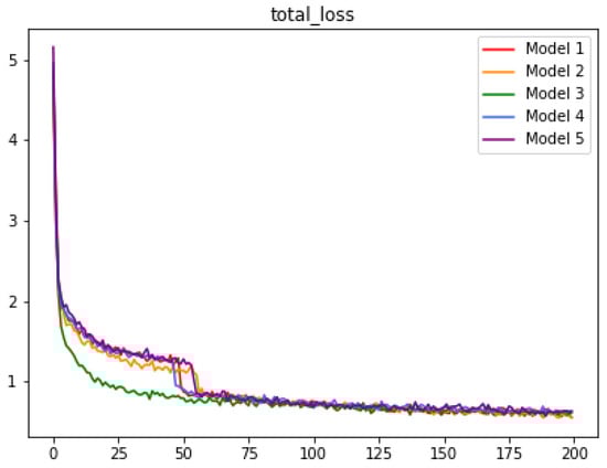
Figure 6. Total training loss of all models, where x-axis represents epoch time.

We notice that some blood cells on the input images are unclear and heavily overlap with each other. The background-like color further causes the successful detection to be difficult. To investigate the performance of the five models in depth, we selected a representative image of each kind of blood cell and discussed the experiment results.

We must note that the annotation files of the BCCD dataset do not label all of the blood cells for unknown reasons; this has a significant impact on the precision of all of the models.

4.4.1. Red Blood Cell Detection

RBCs comprise the majority of the BCCD dataset. Figure 7 and Figure 8 show images with sparse and overlapping RBCs, respectively, while Table 6 shows the experimental results of the five models under two confidence scores.

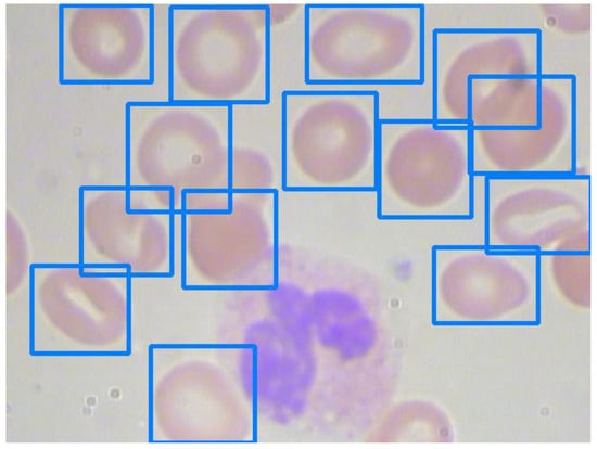
Figure 7. An image with sparse red blood cells.

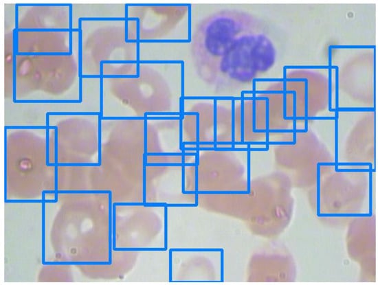
Figure 8. An image with overlapping red blood cells.

Table 6. Comparison of the experiment results between Figure 7, Figure 8, and the validation set.

	Confidence Score: 0.9						Confidence Score: 0.8
Index *	PFig7	RFig7	PFig8	RFig8	Pv	Rv	PFig7	RFig7	PFig8	RFig8	Pv	Rv
Model 1	1	1	0.75	0.429	0.737	0.744	1	1	0.625	0.476	0.693	0.799
Model 2	1	0.929	0.833	0.476	0.794	0.673	1	0.929	0.846	0.524	0.761	0.748
Model 3	0.933	1	0.846	0.524	0.747	0.823	0.875	1	0.813	0.619	0.701	0.867
Model 4	1	1	0.727	0.381	0.731	0.762	0.875	1	0.625	0.476	0.684	0.814
Model 5	1	0.786	1	0.143	0.808	0.517	1	0.786	0.75	0.143	0.763	0.579

* P_Fig7 and R_Fig7 refer to the precision and recall of RBC detection on Figure 7, P_Fig8 and R_Fig8 refer to those on Figure 8, and P_v and R_v refer to those on the validation set.

The models generally can recognize sparse RBCs well and return excellent scores. Nevertheless, their performance depends on their recognition capabilities for overlapping blood cell detection. For example, although Models 3 and 5 have impressive precision for RBC detection, as seen in Figure 8, the differences in recalls between Models 3 and 5 are 38.1% (42.4–14.3%) and 47.6% (61.9–14.3%) under a confidence score of 0.9 and 0.8, respectively. The recalls of RBC detection in Figure 7 and Figure 8 of Model 5 are 78.5% and 14.3%, respectively. As a result, the recall of RBC detection on the validation set of Model 5 is significantly lower than those of the other models. On the other hand, Model 3 still has recalls of 52.4% and 61.9% for RBC detection in Figure 8 under confidence scores of 0.9 and 0.8, respectively.

4.4.2. White Blood Cell Detection

WBC detection is usually the easiest task in blood cell counting due to the size and peculiar color of WBCs. Figure 9 shows an image with two adjacent WBCs. We comprehend the ability of each model in Table 7.

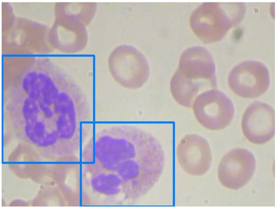
Figure 9. An image with adjacent white blood cells.

Table 7. Comparison of the experiment results between Figure 9 and validation set.

	Confidence Score: 0.9				Confidence Score: 0.8
Index *	PFig9	RFig9	Pv	Rv	PFig9	RFig9	Pv	Rv
Model 1	1	1	0.761	0.95	1	1	0.691	0.964
Model 2	1	1	0.521	0.614	1	1	0.536	0.7
Model 3	1	0.5	0.214	0.2	1	0.5	0.279	0.271
Model 4	1	1	0.704	0.886	1	1	0.662	0.921
Model 5	1	1	0.487	0.936	1	1	0.414	0.95

* P_Fig9 and R_Fig9 refer to the precision and recall of WBC detection on Figure 9, and P_v and R_v refer to those on the validation set.

As shown in Table 7, all of the models, except Model 3, can precisely identify neighboring WBCs, as seen in Figure 9 under confidence scores of 0.9 and 0.8. Model 1 has the best precision and recalls of WBC detection on the validation set.

4.4.3. Platelets Detection

Platelets are smaller than RBCs and WBCs. Furthermore, platelets are significantly fewer than RBCs and WBCs. As a result, platelet detection is always the hardest task in blood cell counting, especially when the platelets are clustered. We take Figure 10 and Figure 11 as examples for investigation. The experiment results are shown in Table 8.

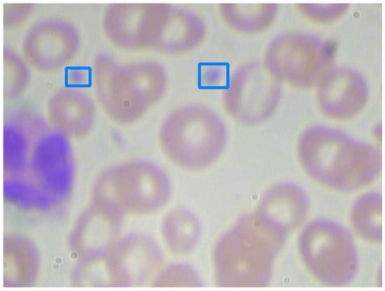
Figure 10. An image with unobvious platelets.

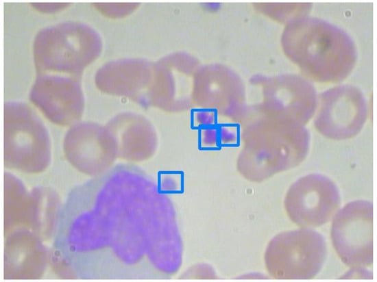
Figure 11. An image with clustered platelets.

Table 8. Comparison of the experiment results between Figure 10, Figure 11, and validation set.

	Confidence Score: 0.9						Confidence Score: 0.8
Index *	PFig10	RFig10	PFig11	RFig11	Pv	Rv	PFig10	RFig10	PFig11	RFig11	Pv	Rv
Model 1	1	0.5	1	0.25	0.498	0.412	1	0.5	1	0.25	0.508	0.53
Model 2	1	1	1	0.25	0.529	0.429	1	1	0.5	0.25	0.47	0.67
Model 3	0	0	0	0	0.382	0.288	1	0.5	0	0	0.453	0.576
Model 4	1	1	0	0	0.381	0.431	1	1	0.333	0.25	0.351	0.518
Model 5	0	0	0	0	0.114	0.067	0	0	0	0	0.14	0.116

* P_Fig10 and R_Fig10 refer to the precision and recall of platelet detection on Figure 10, P_Fig11 and R_Fig11 refer to those on Figure 11, and P_v and R_v refer to those on the validation set.

As shown in Figure 10, platelets are small and unobvious. After enlarging the input images by 1.25 times and preprocessing, Model 2 can successfully recognize them. However, in Figure 11, three platelets are clustered. As shown in Table 8, they cannot be recognized separately, even by the best Model 2. Model 5 performs significantly worse than all of the others. This reveals the disadvantage of only using RGB images.

4.4.4. Summary

RBCs comprise the majority of the BCCD dataset. When RBCs are dense and heavily overlapping, RBC detection becomes harder. With suitable preprocessing and the enlargement of input images, Model 3 performs outstandingly. Model 5, which only uses RBG images, has high precision for RBC detection; however, its recalls on overlapped RBC detection are significantly reduced.

WBCs are larger than RBCs and Platelets. WBC detection is usually an easier task in blood cell counting. With suitable preprocessing, Model 1 outperforms other models, even when the WBCs are neighboring.

Platelets are few and small. Platelet detection is always the hardest task in blood cell counting, especially when platelets are clustered. With the proper enlargement of the input images, Model 2 performs better than the others.

5. Conclusions

In this paper, we propose a novel CNN-based blood cell detection and counting architecture. In this architecture, we adopt VGG-16 as the backbone. The feature maps generated by VGG-16 are enriched by feature fusion and block attention mechanism (CBAM). The concepts of RPN and RoI Pooling from Faster R-CNN are used for blood cell detection. We used the BCCD dataset of blood smear images for the performance evaluation of the proposed architecture. The original images were preprocessed, including image augmentation, enlargement, sharpening, and blurring. Five models with different settings were constructed. The experiments on the RBCs, WBCs, and platelets detection were performed under two confidence scores: 0.9 and 0.8, respectively.

For RBC detection, Model 3, which enlarges input images 1.5-fold and uses images in both RGB and grayscale color spaces, achieved the best recalls: 82.3% and 86.7% under two confidence scores: 0.9 and 0.8, respectively. Meanwhile, it achieved a precision of 74.7% and 70.1% under the two confidence scores. Model 5, which uses RBG images only, scores with an impressive precision; however, it also scores notorious recalls, especially when RBCs are heavily overlapping.

WBC detection is usually the easiest task in blood cell counting due to the size and peculiar color of WBCs. For WBC detection, Model 1, which performs image preprocessing and uses both RBG and grayscale images, outperforms other models. The precision and recall are 76.1% and 95%, respectively, under a confidence score of 0.9, and 69.1% and 96.4%, respectively, under a confidence score of 0.8.

Platelets are smaller and fewer than RBCs and WBCs. Platelet detection is harder than RBC and WBC detections, especially when the platelets are clustered.

We note that the annotation files of the BCCD dataset do not label all of the blood cells due to unknown reasons, significantly impacting the precision of all the models.

Future Work

In blood smear images, some blood cells are at the edge of the images. We are currently working on improving our architecture with the concept introduced in Mask R-CNN [50] to handle imperfect blood cells. As well, recent deep learning object detection models are under consideration. We also look for more datasets of blood smear images to include more blood cell samples for learning.

References

- Habibzadeh, M.; Krzyżak, A.; Fevens, T. White Blood Cell Differential Counts Using Convolutional Neural Networks for Low Resolution Images. In Proceedings of the International Conference on Artificial Intelligence and Soft Computing, Zakopane, Poland, 9–13 June 2013; pp. 263–274. [Google Scholar]
- Wang, W.; Yang, Y.; Wang, X.; Wang, W.; Li, J. Development of convolutional neural network and its application in image classification: A survey. Opt. Eng. 2019, 58, 040901. [Google Scholar] [CrossRef]
- Premaladha, J.; Ravichandran, K.S. Novel approaches for diagnosing melanoma skin lesions through supervised and deep learning algorithms. J. Med. Syst. 2016, 40, 96. [Google Scholar] [CrossRef] [PubMed]
- Liu, W.; Wang, Z.; Liu, X.; Zeng, N.; Liu, Y.; Alsaadi, F.E. A survey of deep neural network architectures and their applications. Neurocomputing 2017, 234, 11–26. [Google Scholar] [CrossRef]
- Alam, M.M.; Islam, M.T. Machine learning approach of automatic identification and counting of blood cells. Healthc. Technol. Lett. 2019, 6, 103–108. [Google Scholar] [CrossRef] [PubMed]
- Acharjee, S.; Chakrabartty, S.; Alam, M.I.; Dey, N.; Santhi, V.; Ashour, A.S. A semiautomated approach using GUI for the detection of red blood cells. In Proceedings of the International Conference on Electrical, Electronics, and Optimization Techniques, Chennai, India, 3–5 March 2016; pp. 525–529. [Google Scholar]
- Lou, J.; Zhou, M.; Li, Q.; Yuan, C.; Liu, H. An automatic red blood cell counting method based on spectral images. In Proceedings of the 9th International Congress on Image and Signal Processing, BioMedical Engineering and Informatics, Datong, China, 15–17 October 2016; pp. 1391–1396. [Google Scholar]
- Verso, M.L. The evolution of blood-counting techniques. Med. Hist. 1964, 8, 149–158. [Google Scholar] [CrossRef]
- Davis, B.; Kottke-Marchant, K. Laboratory Hematology Practice, 1st ed.; Wiley-Blackwell: Chichester, UK, 2012. [Google Scholar]
- Green, R.; Wachsmann-Hogiu, S. Development, history, and future of automated cell counters. Clin. Lab. Med. 2015, 35, 1–10. [Google Scholar] [CrossRef] [PubMed]
- Graham, M.D. The Coulter principle: Imaginary origins. Cytom. A. 2013, 83, 1057–1061. [Google Scholar] [CrossRef] [PubMed]
- Graham, M.D. The Coulter principle: Foundation of an Industry. J. Lab. Autom. 2003, 8, 72–81. [Google Scholar] [CrossRef]
- Madhloom, H.T.; Kareem, S.A.; Ariffin, H.; Zaidan, A.A.; Alanazi, H.O.; Zaidan, B.B. An automated white blood cell nucleus localization and segmentation using image arithmetic and automatic threshold. J. Appl. Sci. 2010, 10, 959–966. [Google Scholar] [CrossRef]
- Rezatofighi, S.H.; Soltanian-Zadeh, H. Automatic recognition of five types of white blood cells in peripheral blood. Comput. Med. Imaging Graph. 2011, 35, 333–343. [Google Scholar] [CrossRef] [PubMed]
- Acharya, V.; Kumar, P. Identification and red blood cell automated counting from blood smear images using computer-aided system. Med. Biol. Eng. Comput. 2018, 56, 483–489. [Google Scholar] [CrossRef] [PubMed]
- Kaur, P.; Sharma, V.; Garg, N. Platelet count using image processing. In Proceedings of the 3rd International Conference on Computing for Sustainable Global Development, New Delhi, India, 16–18 March 2016; pp. 2574–2577. [Google Scholar]
- Cruz, D.; Jennifer, C.; Valiente; Castor, L.C.; Mendoza, C.M.; Jay, B.; Jane, L.; Brian, P. Determination of blood components (WBCs, RBCs, and Platelets) count in microscopic images using image processing and analysis. In Proceedings of the 9th IEEE International Conference on Humanoid, Nanotechnology, Information Technology, Communication and Control, Environment and Management, Manila, Philippines, 1–3 December 2017; pp. 1–7. [Google Scholar]
- Qayyum, A.; Anwar, S.M.; Majid, M.; Awais, M.; Alnowami, M. Medical image analysis using convolutional neural networks: A review. J. Med. Syst. 2018, 42, 1–13. [Google Scholar]
- Razzak, M.I.; Naz, S.; Zaib, A. Deep learning for medical image processing: Overview, challenges and future. In Classification in BioApps; Lecture Notes in Computational Vision and Biomechanics; Dey, N., Ashour, A., Borra, S., Eds.; Springer: Cham, Switzerland, 2018; Volume 26, pp. 323–350. [Google Scholar]
- Qayyum, A.; Anwar, S.M.; Awais, M.; Majid, M. Medical image retrieval using deep convolutional neural network. Neurocomputing 2017, 266, 8–20. [Google Scholar] [CrossRef]
- Su, M.; Cheng, C.; Wang, P. A neural-network-based approach to white blood cell classification. Sci. World J. 2014, 2014, 796371. [Google Scholar] [CrossRef] [PubMed]
- Nazlibilek, S.; Karacor, D.; Ercan, T.; Sazli, M.H.; Kalender, O.; Ege, Y. Automatic segmentation, counting, size determination and classification of white blood cells. Measurement 2014, 55, 58–65. [Google Scholar] [CrossRef]
- Habibzadeh, M.; Jannesari, M.; Rezaei, Z.; Baharvand, H.; Totonchi, M. Automatic white blood cell classification using pre-trained deep learning models: ResNet and Inception. In Proceedings of the SPIE 10696, the 10th International Conference on Machine Vision, Vienna, Austria, 13–15 November 2017; p. 1069612. [Google Scholar]
- Çelebi, S.; Çöteli, M.B. Red and white blood cell classification using Artificial Neural Networks. AIMS Bioeng. 2018, 5, 179–191. [Google Scholar] [CrossRef]
- Hubel, D.H.; Wiesel, T.N. Receptive fields, binocular interaction and functional architecture in the cat’s visual cortex. J. Physiol. 1962, 160, 106–154. [Google Scholar] [CrossRef]
- Fukushima, K.; Miyake, S. Neocognitron: A new algorithm for pattern recognition tolerant of deformations and shifts in position. Pattern Recognit. 1982, 15, 455–469. [Google Scholar] [CrossRef]
- LeCun, Y.; Boser, B.; Denker, J.S.; Henderson, D.; Howard, R.E.; Hubbard, W.; Jackel, L.D. Backpropagation applied to handwritten zip code recognition. Neural Comput. 1989, 1, 541–551. [Google Scholar] [CrossRef]
- Gu, J.; Wang, Z.; Kuen, J.; Ma, L.; Shahroudy, A.; Shuai, B.; Liu, T.; Wang, X.; Wang, G.; Cai, J.; et al. Recent advances in convolutional neural networks. Pattern Recognit. 2018, 77, 354–377. [Google Scholar] [CrossRef]
- LeCun, Y.; Bottou, L.; Bengio, Y.; Haffner, P. Gradient-based learning applied to document recognition. Proc. IEEE 1998, 86, 2278–2324. [Google Scholar] [CrossRef]
- Krizhevsky, A.; Sutskever, I.; Hinton, G.E. ImageNet classification with deep convolutional neural networks. In Proceedings of the 26th Conference on Neural Information Processing Systems, Lake Tahoe, NV, USA, 3–6 December 2012; pp. 1106–1114. [Google Scholar]
- Simonyan, K.; Zisserman, A. Very deep convolutional networks for large-scale image recognition. In Proceedings of the 3rd International Conference on Learning Representations, San Diego, CA, USA, 7–9 May 2015. [Google Scholar]
- Szegedy, C.; Liu, W.; Jia, Y.; Sermanet, P.; Reed, S.; Anguelov, D.; Erhan, D.; Vanhoucke, V.; Rabinovich, A. Going deeper with convolutions. In Proceedings of the IEEE Conference on Computer Vision and Pattern Recognition, Boston, MA, USA, 7–12 June 2015; pp. 1–9. [Google Scholar]
- He, K.; Zhang, X.; Ren, S.; Sun, J. Deep residual learning for image recognition. In Proceedings of the IEEE Conference on Computer Vision and Pattern Recognition, Las Vegas, NV, USA, 27–30 June 2016; pp. 770–778. [Google Scholar]
- Hinton, G.E.; Osindero, S.; Teh, Y.W. A fast learning algorithm for deep belief nets. Neural Comput. 2006, 18, 1527–1554. [Google Scholar] [CrossRef]
- Khan, A.; Sohail, A.; Zahoora, U.; Qureshi, A.S. A survey of the recent architectures of deep convolutional neural networks. Artif. Intell. Rev. 2020, 53, 5455–5516. [Google Scholar] [CrossRef]
- Girshick, R.; Donahue, J.; Darrell, T.; Malik, J. Rich feature hierarchies for accurate object detection and semantic segmentation. In Proceedings of the IEEE Conference on Computer Vision and Pattern Recognition, Columbus, OH, USA, 23–28 June 2014; pp. 580–587. [Google Scholar]
- Uijlings, J.R.; van de Sande, K.E.; Gevers, T.; Smeulders, A.W. Selective search for object recognition. Int. J. Comput. Vis. 2013, 104, 154–171. [Google Scholar] [CrossRef]
- Sermanet, P.; Eigen, D.; Zhang, X.; Mathieu, M.; Fergus, R.; LeCun, Y. OverFeat: Integrated recognition, localization and detection using convolutional networks. In Proceedings of the 2nd International Conference on Learning Representations, Banff, AB, Canada, 14–16 April 2014. [Google Scholar]
- Girshick, R.B. Fast R-CNN. In Proceedings of the IEEE International Conference on Computer Vision, Santiago, Chile, 7–13 December 2015; pp. 1440–1448. [Google Scholar]
- Cao, C.; Wang, B.; Zhang, W.; Zeng, X.; Yan, X.; Feng, Z.; Liu, Y.; Wu, Z. An improved faster R-CNN for small object detection. IEEE Access 2019, 7, 106838–106846. [Google Scholar] [CrossRef]
- Ren, S.; He, K.; Girshick, R.; Sun, J. Faster R-CNN: Towards real-time object detection with region proposal networks. IEEE Trans. Pattern Anal. Mach. Intell. 2015, 39, 1137–1149. [Google Scholar] [CrossRef]
- Zhu, Y.; Zhang, C.; Zhou, D.; Wang, X.; Bai, X.; Liu, W. Traffic sign detection and recognition using fully convolutional network guided proposals. Neurocomputing 2016, 214, 758–766. [Google Scholar] [CrossRef]
- Mangai, U.G.; Samanta, S.; Das, S.; Chowdhury, P.R. A survey of decision fusion and feature fusion strategies for pattern classification. IETE Tech. Rev. 2010, 27, 293–307. [Google Scholar] [CrossRef]
- Woo, S.; Park, J.; Lee, J.; Kweon, I.S. CBAM: Convolutional block attention module. In Proceedings of the European Conference on Computer Vision, Munich, Germany, 8–14 September 2018; pp. 3–19. [Google Scholar]
- Jaccard, P. Etude comparative de la distribution florale dans une portion des Alpes et des Jura. Bull. De La Société Vaud. Des Sci. Nat. 1901, 37, 547–579. [Google Scholar]
- Zheng, Z.; Wang, P.; Liu, W.; Li, J.; Ye, R.; Ren, D. Distance-IoU loss: Faster and better learning for bounding box regression. In Proceedings of the AAAI Conference on Artificial Intelligence, New York, NY, USA, 7–12 February 2012; pp. 12993–13000. [Google Scholar]
- Blood Cell Count and Detection. Available online: https://github.com/Shenggan/BCCD_Dataset (accessed on 1 August 2002).
- Krishna, H.; Jawahar, C.V. Improving small object detection. In Proceedings of the 4th IAPR Asian Conference on Pattern Recognition, Nanjing, China, 26–29 November 2017; pp. 340–345. [Google Scholar]
- Gonzalez, R.C.; Woods, R.E. Digital Image Processing, 4th ed.; Pearson Education: Harlow, UK, 2018. [Google Scholar]
- He, K.; Gkioxari, G.; Dollár, P.; Girshick, R.B. Mask R-CNN. In Proceedings of the IEEE International Conference on Computer Vision, Venice, Italy, 22–29 October 2017; pp. 2980–2988. [Google Scholar]
Publisher’s Note: MDPI stays neutral with regard to jurisdictional claims in published maps and institutional affiliations. |
© 2022 by the authors. Licensee MDPI, Basel, Switzerland. This article is an open access article distributed under the terms and conditions of the Creative Commons Attribution (CC BY) license (https://creativecommons.org/licenses/by/4.0/).