A Two-Stage Decomposition-Reinforcement Learning Optimal Combined Short-Time Traffic Flow Prediction Model Considering Multiple Factors

Abstract

Accurate short-term traffic flow prediction is a prerequisite for achieving an intelligent transportation system to proactively alleviate traffic congestion. Considering the complex and variable traffic environment, so that the traffic flow contains a large number of non-linear characteristics, which makes it difficult to improve the prediction accuracy, a combined prediction model that reduces the unsteadiness of traffic flow and fully extracts the traffic flow features is proposed. Firstly, decompose the traffic flow data into multiple components by the seasonal and trend decomposition using loess (STL); these components contain different features, and the optimized variational modal decomposition (VMD) is used for the second decomposition of the component with large fluctuation frequencies, and then the components are reconstructed according to the fuzzy entropy and Lempel-Ziv complexity index and the Pearson correlation coefficient is used to filter the traffic flow features. Then light gradient boosting machine (LightGBM), long short-term memory with attention mechanism (LA), and kernel extreme learning machine with genetic algorithm optimization (GA-KELM) are built for prediction. Finally, we use reinforcement learning to integrate the advantages of each model, and the weights of each model are determined to obtain the best prediction results. The case study shows that the model established in this paper is better than other models in predicting urban road traffic flow, with an average absolute error of 2.622 and a root mean square error of 3.479, both of which are lower than the prediction errors of other models, indicating that the model can fully extract the features in complex traffic flow.

1. Introduction

With the rapid development of the global economy, car ownership and people’s travel demands have gradually increased, thus bringing huge challenges to urban traffic [1]. To alleviate urban traffic congestion and reduce the hazards caused by traffic congestion, traffic managers have proposed the following solutions: (1) Expansion of existing urban roads and other infrastructure, thereby increasing the capacity of the roads. However, in urban planning, the limited area of land use makes it difficult to build urban infrastructure to meet traffic demands, and some studies have shown that road expansion only relieves traffic congestion in the short term [2]; however, according to the theory of supply and demand, the potential traffic demand will increase, leading to a more serious traffic congestion problem [3]. (2) Establish an intelligent transportation system (ITS) that applies information, communication, sensor, and computer technologies to road traffic guidance and management. Road managers dynamically adjust control methods through real-time traffic status to improve road management [4], and ITS can provide road congestion information for travelers to choose a reasonable route out and improve travel efficiency, so it is vital for relieving urban traffic congestion ITS, and traffic flow prediction is the key for ITS to achieve active services, which can provide accurate real-time traffic information for ITS.

Traffic flow prediction refers to the prediction of traffic flow in a future period by historical traffic flow information, from the initial statistical learning models, nonlinear theoretical methods, and shallow neural network models to the current large-scale use of deep learning methods and statistical models through the periodic patterns in historical data for prediction; the theory is simple, but it is difficult to deal with the dynamic changes in traffic flow data. Shallow neural networks have limitations in the face of larger data samples [5], and the traffic system is highly susceptible to interference from the external environment, resulting in a large number of nonlinear features in the traffic flow [6], and a single model cannot handle both linear and nonlinear features in the traffic flow, so a combined prediction model is necessary to improve the prediction accuracy. Traffic flow data are not only correlated in time, with a certain regularity in continuous periods, but also correlated in space due to the topology of the traffic network, and the current cross-section traffic flow is influenced by the upstream and downstream traffic states. The model is easier to capture the potential features of the unsteady traffic flow data by decomposing the data to obtain multiple smoother components. For this reason, Ma et al. [7] define that a good traffic flow prediction method should have the following characteristics: (1) ensure that the model completely extracts the salient features in the traffic flow, (2) be able to consider the spatio-temporal correlation of traffic flow in the road network, and (3) analyze the influencing factors of traffic changes. However, in the past studies on short-term traffic flow prediction, some studies considered the spatio-temporal correlation between external environmental factors and traffic flow without analyzing the potential features in traffic flow; some studies analyzed from the perspective of traffic flow decomposition, but ignored the connection between traffic flow features, while this paper is dedicated to combining the two, using the decomposition method to reduce the unsteadiness of traffic flow and fully considering the spatio-temporal characteristics of traffic flow based on this, we propose two-level decomposition-reinforcement learning optimized combined short-time traffic flow prediction model considering multiple factors. Firstly, the model has two-stage decomposition by STL and VMD, and scientific reconstruction of each component using fuzzy entropy and the Lempel-Ziv complexity index to improve operational efficiency. Secondly, the spatio-temporal and external features affecting traffic flow are selected by Pearson correlation coefficients for features. Furthermore, the obtained components fused with external features are established as LightGBM, LA, and GA-KELM for prediction. Finally, the weights of each model are optimized using reinforcement learning to obtain the predicted values of traffic flow.

The rest of the paper is organized as follows: Section 2 is a literature review. In Section 3, the two-stage decomposition approach (STL and VMD), the rationale of the three prediction models, and the Q-learning algorithm for optimizing the combined weights, as well as a detailed description of the model structure and process, are included. Section 4 performs a real case study analysis and analyzes and validates the effectiveness of the approach through ablation experiments and model comparisons. Section 5 outlines the conclusions obtained.

2. Literature Review

Advanced traveler information systems and advanced traffic management systems in ITS can actively control traffic signals and actively induce congested traffic flow through predicted traffic flow information [8]; they can aid in passive signal control through real-time traffic flow information [9] when the traffic flow is too large and it is difficult to ensure the smooth flow of the road, and the prediction of the traffic flow for some time in the future can predict the state of the road section, so that traffic managers can control the converging traffic flow in advance, thus reducing the possibility of congestion. For automatic driving technology, the traffic density of the approaching road section can be predicted in advance, and when the density is high, the automatic driving vehicle can reduce the speed and other measures in advance to improve driving safety [10], and can reduce the travel time by predicting the congestion state of the road section in advance and doing route planning.

Disturbed by the external environment, the urban traffic system becomes complex and variable, and factors such as weather and morning and evening peaks can affect traffic flow in a nonlinear relationship [11]. Compared with medium-term and long-term traffic flow forecasting, short-term traffic flow forecasting has a shorter time granularity, and the obtained traffic flow data are more random, making short-term traffic flow forecasting more challenging [12,13]. Forecasting methods are mainly parametric and non-parametric models, and parametric models are statistical class models [14] and Kalman filter models [15]; to capture the seasonal variation of macroscopic traffic flow, Williams et al. [16] proposed the seasonal autoregressive integrated moving average model. However, such shallow models are suitable for relatively smooth and small sample data, which require high data quality and are difficult to accurately fit the changes of complex traffic flow; non-parametric models mainly include tree models and neural network models [17]. Li et al. [18] applied to the prediction of traffic flow with high accuracy by building a Support Vector Regression (SVR) model and optimizing its parameters. Zhang et al. [19] established a combined prediction model of the LSTM and the extreme gradient boosting (XGBoost) for the temporal characteristics of traffic flow data, fused the advantages of the two models, replaced the fully connected layer of LSTM with XGBoost, and validated the model using the data from Shenzhen. The commonly used neural network models are Back Propagation Neural Network [20], radial basis function neural network [21], and wavelet neural network models [22,23], which essentially use error backpropagation to modify the weights to fit the data, but are highly susceptible to fall into local optimal solutions and have limited feature capture capability.

To adapt to the current data era, researchers at home and abroad have favored the use of data-driven models based on deep learning to predict short-time traffic flow [24], and it has been found that the combined models can avoid the problem of inadequate feature capture capability of a single model [25,26], with higher prediction accuracy and better generalization capability. Considering the spatio-temporal characteristics of traffic flow and the interference of the external environment on traffic flow, Wang et al. [27] propose a One-Dimensional Convolutional Neural Network (1DCNN) and LSTM model combined with an attention mechanism. The 1DCNN is used to extract spatial features in the road, then input to LSTM to extract temporal features, and use the attention mechanism to extract key features; the simulation analysis shows that the model has better prediction results. Wang et al. [28] considered the complexity of traffic flow, differenced the reconstructed data to make the data smoother, and used a combined model of recurrent neural network and LSTM for prediction; Zheng et al. [29] built a hybrid prediction model, modeled separately according to different features, and introduced an attention module to adaptively assign feature weights.

The traffic system is extremely time varying and shows a certain periodicity in the time sequence; there is a dependency between the current traffic state change and the historical traffic state [30], and the network topology of traffic makes the traffic flow of adjacent sections affect the target section [31]. Ali et al. [32] proposed a deep spatio-temporal neural network based on the spatio-temporal characteristics of traffic flow, which consists of predicting the spontaneous variation part of traffic flow, the periodic part, and the external features part, and the model predicts better with other models established wavelet. The external environment affects the traffic system all the time [33], making it highly uncertain, so the integration of external features is necessary to achieve accurate traffic flow prediction. Lin et al. [34] explored the influence of three external features of time, weather, and day of the week on traffic flow, and input the features into the gradient-boosted decision tree (GBDT) model for prediction, where the experimental results verified the feasibility of the method. Ji et al. [35] established an LSTM-SVR model based on the influence of holidays on highway traffic flow, and they used LSTM to extract features from holiday data and input them into the SVR model for prediction. Li et al. [36] used CNN to extract spatial features, LSTM, and the gated recurrent unit to extract temporal features; built models for weekday and holiday prediction; and verified the prediction accuracy of the models, but such models containing temporal memory units are difficult to tap potential features in discontinuous data.

For the decomposition-integration model, Huang et al. [37] compared the effects of different decomposition methods, such as empirical mode decomposition (EMD), VMD, and wavelet decomposition (WD), on the prediction effect; obtained the components containing different features by clustering; and finally predicted each component by a two-way long and short-term memory neural network. However, the influence of external factors on the traffic flow was not considered, and there were a large number of unsteady features in the high-frequency components obtained from the decomposition, as well as the limited ability of a single model to capture potential features in the traffic flow [38], Zhao et al. [39] decomposed the traffic flow data using STL, extracted spatial and temporal features using CNN and LSTM, respectively, introduced the attention mechanism to assign feature weights, and finally weighted and summed the predicted values of each component.

3. Methods

3.1. Two-Stage Decomposition

First stage decomposition method: Smoothing the sequence $y$ by STL decomposition [40], adjusting the robustness weights of Loess in the inner loop using the outer loop, and the complete detrending and cycling of sequences in inner loops is performed to obtain the trend component $Y_t$ and the period component $Y_c$, while the residual component $Y_r$ consists of the remaining values of the original sequence. The expression is as follows:

$$y=f(Y_t,Y_c,Y_r)$$

(1)

STL can break down practically any data with periodicity, is less impacted by missing and aberrant data, and has higher robustness when compared to decomposition techniques like X-11 and SEATS.

It is usually considered that the time series can be decomposed into three components: a deterministic component, a periodic component, and a volatile component [41]. The urban traffic flow is a time series with stable changes and accompanied by some random disturbances [42], due to the inherent characteristics of the traffic flow, such as road attributes and the geographical location where the road is located, which makes the traffic flow have a long-term trend; the travel plans of traffic participants, such as going out plans, such as going out to work and going to school on working days, make the traffic flow have a relatively fixed periodicity; changes in the traffic environment, such as adverse weather conditions and traffic anomalies, lead to sudden changes in the traffic flow state. STL is used to decompose the traffic flow data and then extract the trend and periodic features in the traffic flow. Two common decomposition models of STL are the additive model and multiplicative model; for the inherent trend component and the fluctuation of the periodic component, which do not follow the change of time, choose the additive model; when the trend component follows the change of time with fluctuation changes, choose the multiplicative model, and considering the trend of the traffic flow determined by its intrinsic characteristics, the additive model should be selected.

Second stage decomposition method: The EMD interpolates the extreme points found from the sequence into the upper and lower envelopes, then subtracts the original sequence from the mean of the envelope to obtain a new sequence, and keeps updating it continuously when the difference between the number of extreme points and the number of over zero points is less than one or the mean of the envelope is zero, which indicates that intrinsic mode function (IMF) components are smooth, and stops the above operation. VMD greatly reduces the probability of such problems and makes it adaptive and more fault tolerant, so VMD is chosen for the secondary decomposition of traffic flow.

VMD decomposes a non-smooth time series by setting the number $k$ of band-limited intrinsic mode functions (BIMF) and the quadratic penalty factor $\alpha$. The principle is to transform the variational constrained problem into an unconstrained variational problem; the transformation process needs to satisfy that the sum of the bandwidths of each BIMF is minimum, and the summed sequence is equal to the original sequence; based on Wiener filtering, the original sequence is decomposed into $k$ BIMFs to ensure that the estimated broadband sum of each component is at a minimum, and the specific derivation process of the VMD algorithm is described in Reference [43].

After the traffic flow sequence is decomposed by STL, the residual components with high frequency are obtained. Considering that there are still potential features that are not smooth, and thus interfere with the prediction effect of the model, VMD is used to decompose the residual components twice to fully exploit the useful information in them. The steps regarding the decomposition of the traffic flow by VMD are as follows.

(1)

Construct the variational constraint problem.

$$\{\begin{array}{c}\underset{\left\{u_k\right\},\left\{{\omega }_k\right\}}{\min }\left\{{\displaystyle \sum _k{\Vert {\partial }_t\left[\left(\delta \left(t\right)+\frac{j}{\pi t}\right)\ast u_k(t)\right]e^{-j{\omega }_{h}t}\Vert }_2^2}\right\}\\ {\displaystyle \sum _k{u}_k=f}\end{array}$$

(2)

where $\left\{u_k\right\}$ and $\left\{{\omega }_k\right\}$ are the respective modal functions and the corresponding central frequencies, and $f$ is the sum of each modal function sequence.

(2)

Add a quadratic penalty factor $\alpha$ and Lagrange operator $\lambda$ to the original problem, so that the constrained variational problem becomes an unconstrained variational problem, which is as follows:

$$L\left(\left\{u_k\right\},\left\{{\omega }_k\right\},\lambda \right):=\alpha {{\displaystyle \sum _k\Vert {\partial }_t\left[\left(\delta \left(t\right)+\frac{j}{\pi t}\right)\ast u_k\left(t\right)e^{-j{\omega }_{k}t}\right]\Vert }}_2^2+{\Vert f\left(t\right)-{\displaystyle \sum _k{u}_k\left(t\right)}\Vert }_2^2+\langle \lambda \left(t\right),f\left(t\right)-{\displaystyle \sum _k{u}_k\left(t\right)}\rangle$$

(3)

(3)

Optimize the unconstrained variational problem, and using the alternating direction multiplier algorithm to obtain ${\omega }_k$ and $u_k$ in Equation (3), and iteratively update ${\omega }_k$, $u_k$ and $\lambda$ in the frequency domain.

(4)

The iteration ends when the following conditions are satisfied.

$$\frac{{\displaystyle \sum _k{\Vert {\widehat{u}}_k^{n+1}-{\widehat{u}}_k^n\Vert }_2^2}}{{\Vert {\widehat{u}}_k\Vert }_2^2}<r$$

(4)

where $r$ is the accuracy threshold.

The effectiveness of VMD for traffic flow sequence decomposition depends largely on the setting of the following two parameters: the number of BIMFs $k$ and the quadratic penalty factor $\alpha$. When $k$ is larger or smaller, it will lead to over or under decomposition of the decomposition, and when it is not set properly, the modal mixing phenomenon will occur. 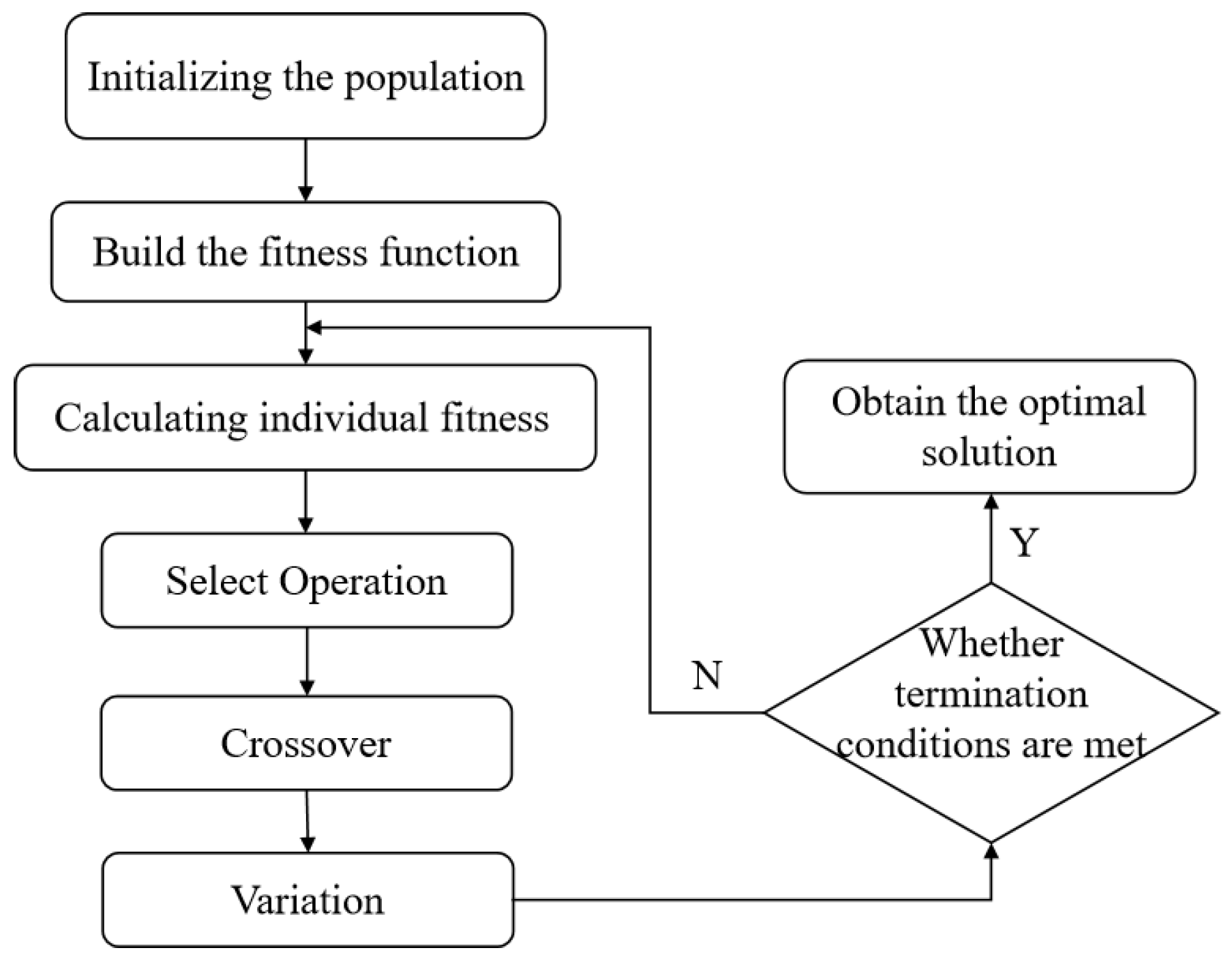It is difficult to set $k$ and $\alpha$ artificially make the VMD achieve the best decomposition, so the optimal combination $[k,\alpha ]$ is solved by using GA with the envelope entropy as the fitness function, the workflow of GA is shown in Figure 1.

3.2. GA Optimized Kernel Extreme Learning Machine

KELM is an improved algorithm of the extreme learning machine (ELM). KELM replaces the random mapping in the hidden layer of ELM with the stable mapping of the kernel function, and the model has stronger generalization and stability, the formula for KELM is as follows:

$$f\left(x\right)=\left[\begin{array}{c}K\left(x,x_1\right)\\ ⋮\\ K\left(x,x_n\right)\end{array}\right]{\left(\frac{I}{C}+{\mathsf{\Omega }}_{ELM}\right)}^{-1}T$$

(5)

where $K\left(x,x_n\right)$ is the kernel function, $C$ and $I$ are the regularization parameters and the diagonal matrix, respectively, ${\mathsf{\Omega }}_{ELM}$ is the kernel matrix, and $T$ is the target matrix.

Considering that the kernel parameters $\sigma$ and $C$, the model determines the generalization ability and the fitting effect of the model, respectively, and the GA is used to find the two parameters to ensure the prediction effect of KELM.

3.3. Light Gradient Boosting Machine

LightGBM divides continuous features by histogram partitioning based on GBDT, which is more efficient than GBDT. LightGBM works by integrating a certain number of weak regression trees to obtain a strong regression tree, which is used to fit the output of the model, and the specific formula is as follows:

$$F\left(x\right)={\displaystyle \sum _{i=1}^N{f}_i(x)}$$

(6)

where $N$ is the number of weak regression trees, and $f_i(x)$ is the output of the $i$ weak regression trees. Its leaf-wise splitting strategy is to build the tree model by finding the splitting gain of all leaves and choosing the direction with the largest gain to split, thus ensuring the high efficiency of the model computation, reducing the computer memory usage, and making the model still have high performance when dealing with large samples.

3.4. LSTM-Attention Model

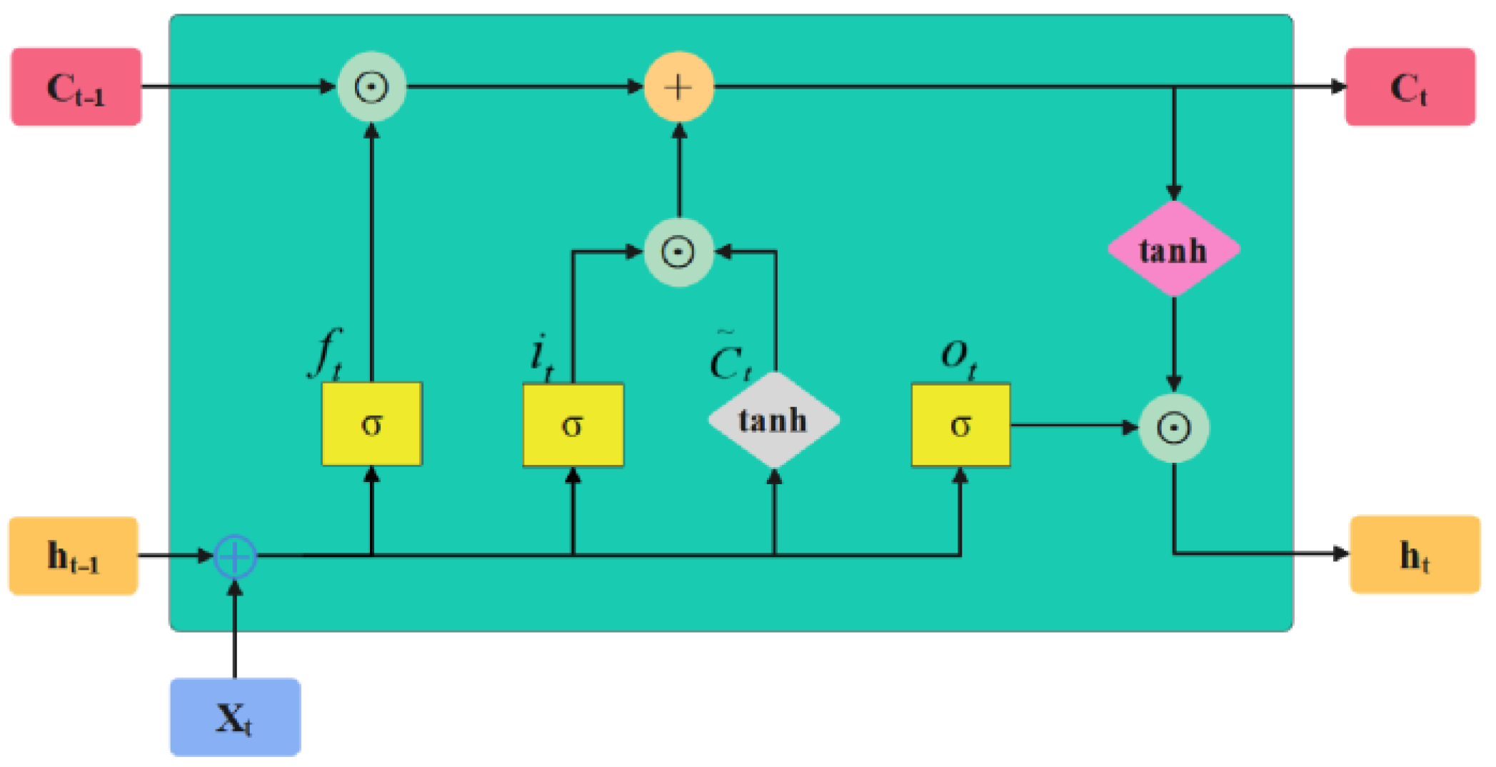
RNN saves all the information when training with data, and the nodes of each hidden layer are linked to each other, thus creating the gradient disappearance and gradient explosion problems [44], while a variant of RNN, LSTM, introduces “gates” to control the path of information propagation, which can effectively suppress such problems; its structure is shown in Figure 2.

The equations for their corresponding doors are as follows:

$$\{\begin{array}{c}{i}_t=\sigma \left(W_i[x_t,h_{t-1}]+b_i\right)\\ f_t=\sigma \left(W_f[x_t,h_{t-1}]+b_f\right)\\ o_t=\sigma \left(W_o[x_t,h_{t-1}]+b_o\right)\end{array}$$

(7)

where $i_t$, $f_t$, and $o_t$ are forgetting gates, input gates, and output gates, which serve to control the forgetting of internal information, the preservation of candidate state information, and the output of internal state information, respectively; $\sigma$ is the activation function; $W$ is the weight of each gate; $x_t$ and $h_{t-1}$ are the input samples of the layer $t$ structure and the memory information of the layer $t-1$ structure, respectively; and $b$ is the bias. In this paper, the attention mechanism is added after the LSTM model to dynamically adjust the weights of the LSTM output data, the LA model, to further extract the nonlinear features in the traffic flow data and reduce the weights of irrelevant information to improve the model prediction effect.

3.5. Q-Learning

Unlike traditional supervised learning, reinforcement learning (RL) is based on interaction with the environment and adjusts the strategy to obtain the maximum reward. In recent years, RL has been continuously applied to solve combinatorial optimization problems [45]; in this paper, we use the Q-learning algorithm in RL to effectively integrate the advantages of three models, and thus improve the predictive performance of the combinatorial model.

The Q-learning algorithm is a deter strategic time-series difference method; it reduces the gap between reality and expectation by iteratively optimizing the Q-function. The optimization idea of Q-learning is applied to the optimization of the weights of the combinatorial model, whose combinatorial prediction model is as follows:

$$X={\omega }_1{x}_1+{\omega }_2{x}_2+{\omega }_3{x}_3$$

(8)

where $X$ is the combined predicted value; ${\omega }_1$, ${\omega }_2$, and ${\omega }_3$ are the weights of GA-KELM, LightGBM, and LA, respectively; and $x_1$, $x_2$, and $x_3$ are the predicted values of the corresponding models, respectively. The specific steps of optimization are as follows.

Step 1: Build the Q-table. Let its state be $S\left(t\right)$ and the action of the intelligent body in optimizing the weight be $A\left(t\right)$. Build the initialized Q-table. The specific formulas are as follows:

$$S\left(t\right)=\left[{\omega }_1,{\omega }_2,{\omega }_3\right]$$

(9)

$$A\left(t\right)=\left[\mathsf{\Delta }\omega ,-\mathsf{\Delta }\omega \right]$$

(10)

where $\mathsf{\Delta }\omega$ is the amount of weight change.

Step 2: Set the reward mechanism. The mean square error $E$ is the objective function, and the reward and punishment function is $R\left(t\right)$. The specific formulas are as follows:

$$E=\left({\displaystyle \sum _{t=1}^N{\left[\widehat{X}\left(t\right)-X\left(t\right)\right]}^2}\right)/N$$

(11)

$$R\left(t\right)=\{\begin{array}{c}+1+E\left(t-1\right)-E\left(t\right)\left(E\left(t-1\right)\ge E\left(t\right)\right)\\ -1+E\left(t-1\right)-E\left(t\right)\left(E\left(t-1\right)<E\left(t\right)\right)\end{array}$$

(12)

where $\widehat{X}$ is the actual value of traffic flow and $N$ is the sample size.

Step 3: Action selection. To minimize the error, the greedy strategy is used for action selection, where the intelligence has the opportunity to explore externally in addition to selecting actions based on past tests, allowing it to discover more valuable situations. Setting a threshold of 0.9 indicates that the intelligence has a 90% probability of selecting the next action from the maximum state value in the Q-table, and for the remaining cases, the action is selected randomly.

Step 4: Q-table update. Its updated formula is as follows:

$$Q_{new}\left(s,a\right)=Q\left(s,a\right)+\alpha \left[r+\gamma \max Q\left(s^{\prime },a^{\prime }\right)-Q\left(s,a\right)\right]$$

(13)

where $Q_{new}\left(s,a\right)$ is the updated Q-value, $\alpha$ is the learning efficiency set to 0.001, $r$ is the reward received after the action, $\gamma$ is the discount factor set to 0.9, and the maximum number of iterations is 1000.

3.6. Model Building

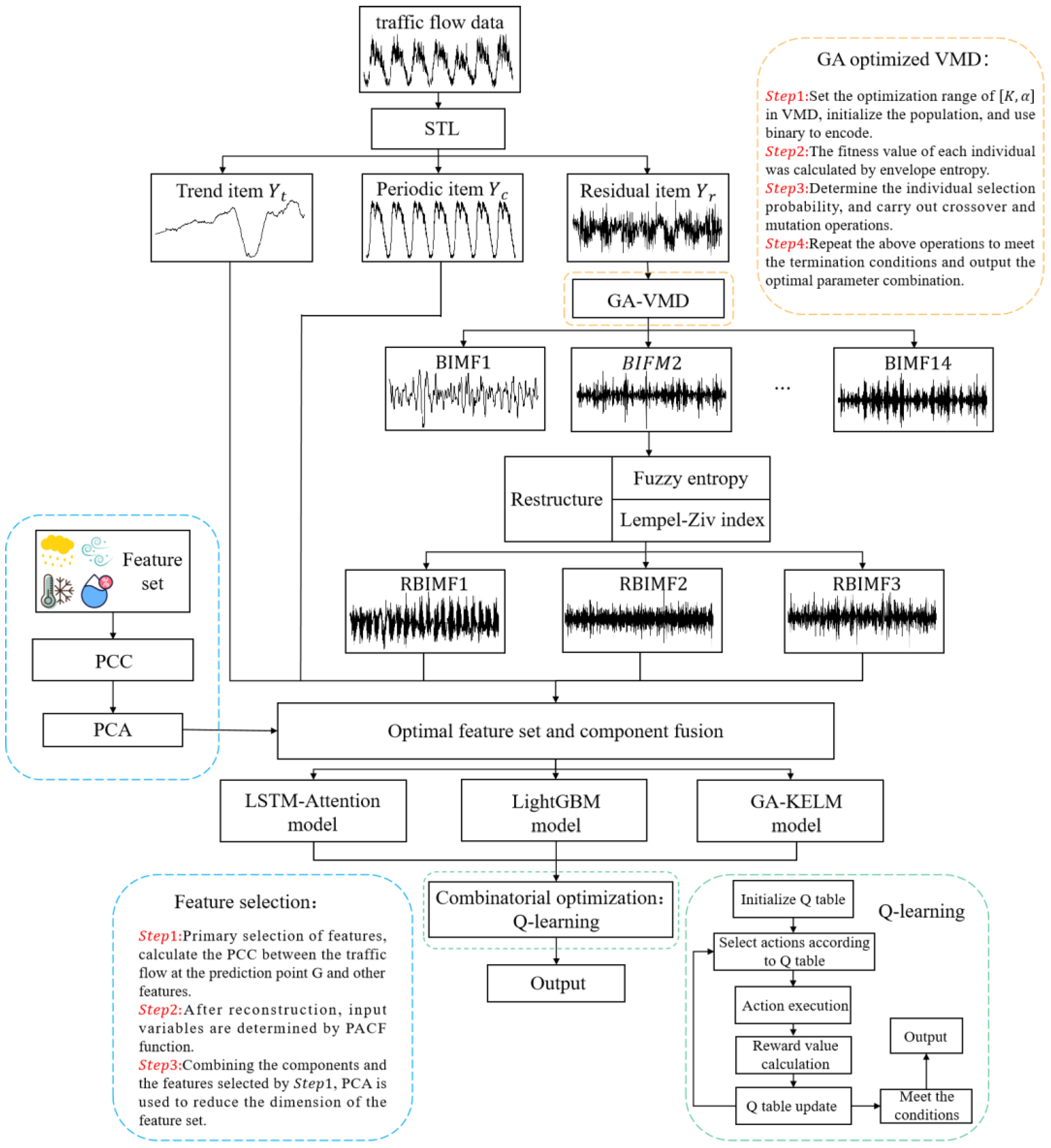
Based on the above discussion, a two-stage decomposition-reinforcement learning optimized short-time traffic flow combination prediction model considering multiple features is proposed, and the process is shown in Figure 3. The unsteadiness of traffic flow is fully reduced by two-stage decomposition, which is beneficial for the model to capture the intrinsic features of traffic flow, and the Q-learning algorithm can effectively integrate the model to improve the prediction accuracy; the specific steps are as follows.

Step1: The data are pre-processed to remove the outliers, and then the missing values are filled.

Step2: The processed data are decomposed by STL to get the trend component, the periodic component, and the residual component, and then the optimized VMD is used to decompose the residual component to get multiple BIMFs.

Step3: The multiple BIMFs are scientifically and reasonably reconstructed by fuzzy entropy and the Lempel-Ziv complexity index.

Step4: The features with greater correlation with traffic flow are selected by using the Pearson coefficient, and the selected features are dimensionalized by the principal component analysis algorithm.

Step5: GA-KELM, LightGBM, and LA are established to predict each component obtained, and Q-learning in reinforcement learning is used to determine the optimal weights of the three models to find the final prediction results.

4. Experiments and Discussion

4.1. Experimental Data

In this paper, the traffic flow data of several road sections in Changsha City from 17 September to 6 October 2019 are used as experimental data, as shown in Figure 4, including the flow data of 13 observation points, denoted by A to M, where G is the road section to be predicted, and the data collection period is 5 min. Then, 288 data are collected daily by a single detector, for a total of 5760 data, and 115,200 data for all detectors. Considering that the data collected by a single detector will have a certain probability of missing values due to its defects and the influence of external environmental factors, the average value of the traffic flow data before and after the missing data is taken to fill it and remove the abnormal values; the traffic flow data of observation points E and F are analyzed to know that there is a large gap with the actual data, so the data of observation points E and F are eliminated, the traffic flow data of 5 and 6 October are used as the test set, and the remaining data are used as the training set.

The required external environmental data were obtained from the Changsha weather detection station, whose latitude and longitude were (112.7833, 28.1166); the collected environmental data were wind speed, temperature, relative humidity, rainfall, and visibility, with a collection interval of 1 h. Their total number was 2400, and some of the data are shown in

Table 1. The data in the external environment section indicates.

Time	Wind Speed (m/s)	Temperature (℃)	Relative Humidity (%)	Rainfall (mm)	Visibility (km)
9/17/0:0:0	2.7	25	84	0	8
9/17/1:0:0	2.7	24.3	85	0	2
9/17/2:0:0	2.7	23.2	86	0	10
9/17/3:0:0	2.7	22.7	86	0	3

.

The time interval of the collected road traffic flow is 5 min, while the interval of the external environmental features collected is 1 h. To match with the traffic flow data, we consider the continuity of environmental changes, so we perform a linear interpolation operation on the environmental data and adjust the time interval to 5 min. To prevent the influence of the magnitude between different features in the prediction, the data are normalized and mapped to the range of [0, 1] uniformly. The formula is as follows.

$$x_i^g=\frac{x_i-x_{\min }}{x_{\max }-x_{\min }}$$

(14)

where $x_i^g$ is the normalized data, $x_i$ is the original traffic flow data, and $x_{\max }$ and $x_{\min }$ are the maximum and minimum values in the traffic flow, respectively.

4.2. Feature Selection

The selection of traffic flow features determines the prediction accuracy to a large extent. The specific traffic features are screened in

Table 2. Set of traffic flow characteristics.

Features	Symbolic Representation	Symbol Meaning	Type
Sequence Features	$\mathrm{G}:\left\{{\mathrm{g}}_1{,\mathrm{g}}_2,\cdots {,\mathrm{g}}_{\mathrm{n}}\right\}$	Predicted traffic flow sequence at point G	Digital
Spatial Features	$\mathrm{A}:\left\{a_1,a_2,\cdots a_n\right\}$ $⋮$ $\mathrm{M}:\left\{m_1,m_2,\cdots m_n\right\}$	The detection points in the road network, except point G Traffic flow sequence	Digital
External Features	$\left\{{\mathsf{\omega }}_{\mathrm{T}}{,\mathsf{\omega }}_{\mathrm{H}}{,\mathsf{\omega }}_{\mathrm{R}}{,\mathsf{\omega }}_{\mathrm{V}}{,\mathsf{\omega }}_{\mathrm{W}}\right\}$	Temperature, relative humidity, rainfall, visibility, and wind speed	Digital
Periodic Features	$\left\{{\mathrm{d}}_1{,\mathrm{d}}_2{,\mathrm{d}}_3\right\}$	Traffic flow at the same moment of the previous day, the average of the first 15 min and 30 min traffic flow	Digital
	$\left\{{\mathrm{S}}_{\mathrm{w}}{,\mathrm{S}}_{\mathrm{h}}{,\mathrm{S}}_{\mathrm{p}}\right\}$	Whether it is a weekday, holiday, or morning and evening peak	Tags

, where the sequence features are the traffic flow of the prediction point, the spatial features are the traffic flow of other detection points in a certain area that influence the prediction point, and the external features are the influence of weather factors on the traffic flow; the periodic features mainly consider the periodicity of days and morning and evening peaks, and whether they are working days and holidays, with the label set to 1 for morning and evening peaks and 0 for the rest of the time. The working day label is set to 1, and the holiday label is set to 1. The time of the morning peak is selected as 8:00–10:00 and the evening peak period is 17:00–20:00.

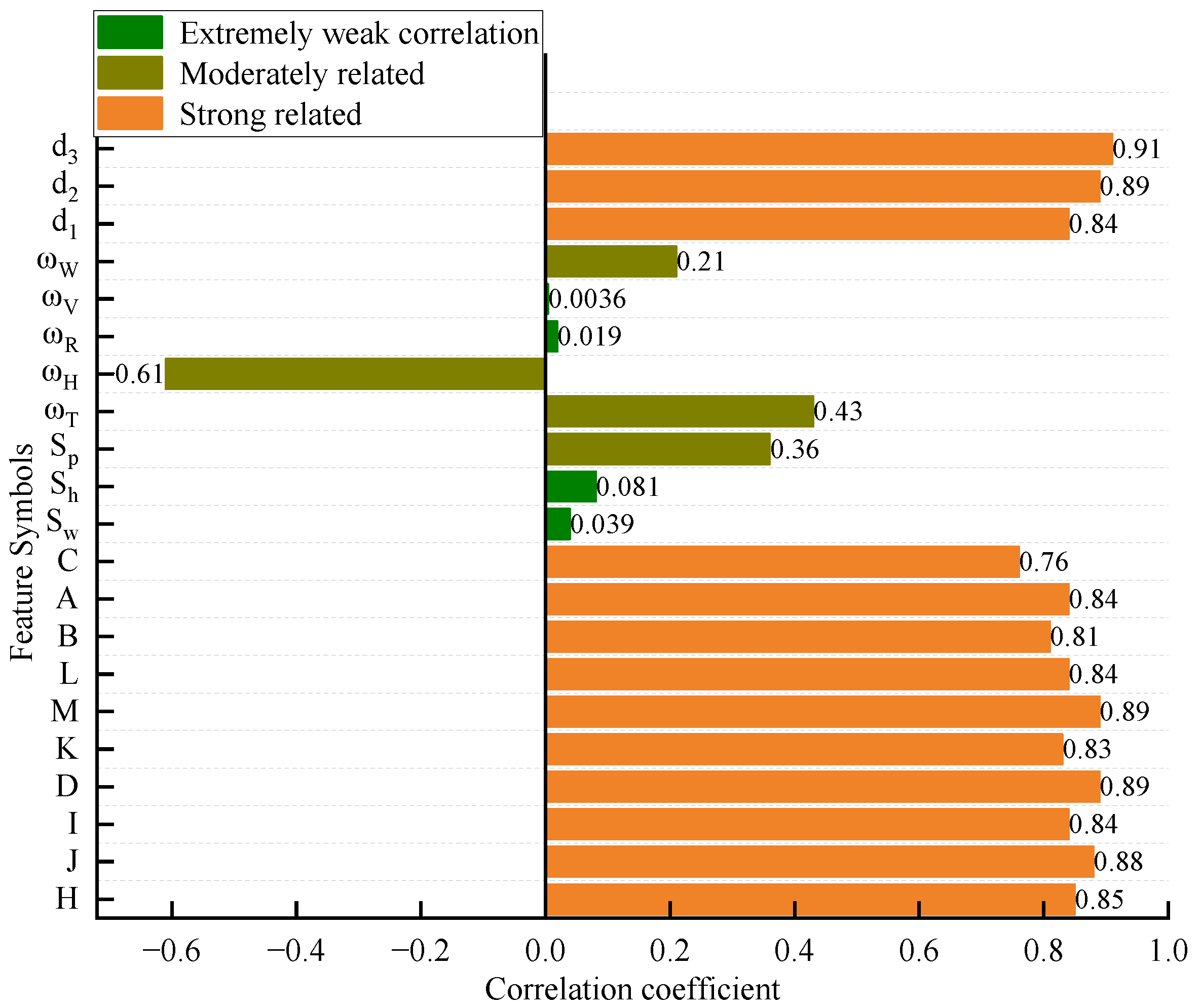
There are many factors affecting traffic flow, but when analyzing traffic flow in a specific environment, each factor has a different degree of influence on traffic flow, and feature selection is required to prevent the introduction of redundant features. Pearson correlation coefficients are used to filter features, and the correlation analysis is shown in Figure 5.

The correlation between the prediction point G and the rest of the road observation points was obtained by analyzing the spatial features, in which the correlation coefficients of E, F and G were 0.18 and 0.087, which are less than 0.2, indicating that the correlation between E, F and G was extremely weak, and by analyzing the traffic flow data of points E and F, it was found that they could not reflect the real traffic conditions, which might be the fault of the detector, and the remaining detection points and G. The correlation coefficients of the remaining detection points with G are all greater than 0.7, and the correlation between them and G is strong; for the external features, the correlation coefficients of ${\mathsf{\omega }}_{\mathrm{T}}$, ${\mathsf{\omega }}_{\mathrm{H}}$, ${\mathsf{\omega }}_{\mathrm{R}}$, ${\mathsf{\omega }}_{\mathrm{V}}$, and ${\mathsf{\omega }}_{\mathrm{W}}$ are 0.43, −0.61, 0.019, 0.0036, and 0.21, respectively, among which the correlation coefficients of ${\mathsf{\omega }}_{\mathrm{R}}$, ${\mathsf{\omega }}_{\mathrm{V}}$, and G are less than 0.2, which is a very weak correlation, ${\mathsf{\omega }}_{\mathrm{W}}$ is a weak correlation, and ${\mathsf{\omega }}_{\mathrm{T}}$ and ${\mathsf{\omega }}_{\mathrm{H}}$ are a medium correlation; the correlation coefficients of ${\mathrm{S}}_{\mathrm{w}}$, ${\mathrm{S}}_{\mathrm{h}}$, ${\mathrm{S}}_{\mathrm{p}}$, ${\mathrm{d}}_1$, ${\mathrm{d}}_2$, ${\mathrm{d}}_3$, and G correlation coefficients can be seen; ${\mathrm{S}}_{\mathrm{w}}$ and ${\mathrm{S}}_{\mathrm{h}}$ are very weakly correlated; ${\mathrm{S}}_{\mathrm{p}}$ is moderately correlated; ${\mathrm{d}}_1$, ${\mathrm{d}}_2$, and ${\mathrm{d}}_3$ are strongly correlated. Thus, ${\mathsf{\omega }}_{\mathrm{R}}$, ${\mathsf{\omega }}_{\mathrm{V}}$, ${\mathrm{S}}_{\mathrm{w}}$, and ${\mathrm{S}}_{\mathrm{h}}$ are removed from the feature set for the accuracy of prediction.

4.3. Traffic Flow Decomposition and Reconfiguration

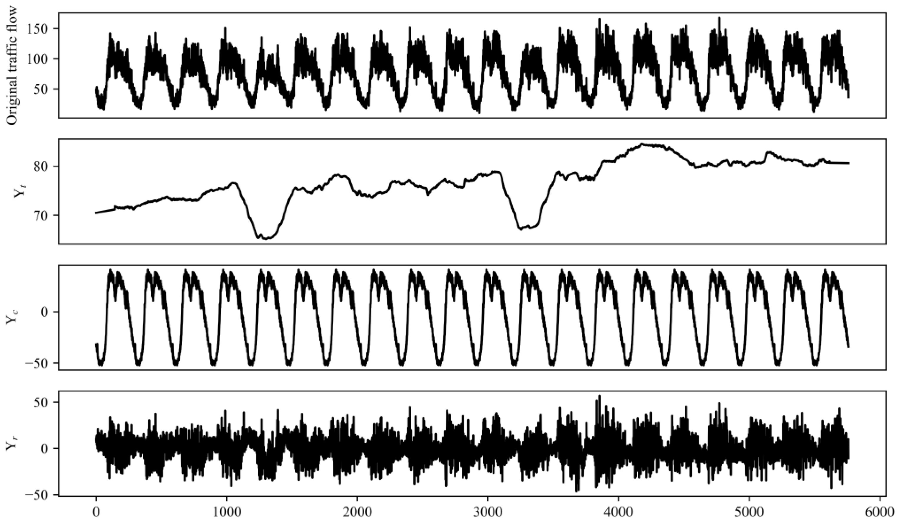
Firstly, the processed traffic flow data are decomposed by STL, and the decomposition results are shown in Figure 6; from the trend term $Y_t$ in the figure, we can see that the overall traffic flow shows an upward trend, and the two depressions correspond to the traffic flow of the weekend, which has a significant decrease. The tail of $Y_t$ is the National Day period, and the demand for going out increases, which leads to a higher traffic flow than the usual period. From the period term $Y_c$, we can see the periodicity of the traffic flow, similar traffic flow changes on a day-to-day basis, and that the traffic flow in the morning and evening peak is higher than the flat period. 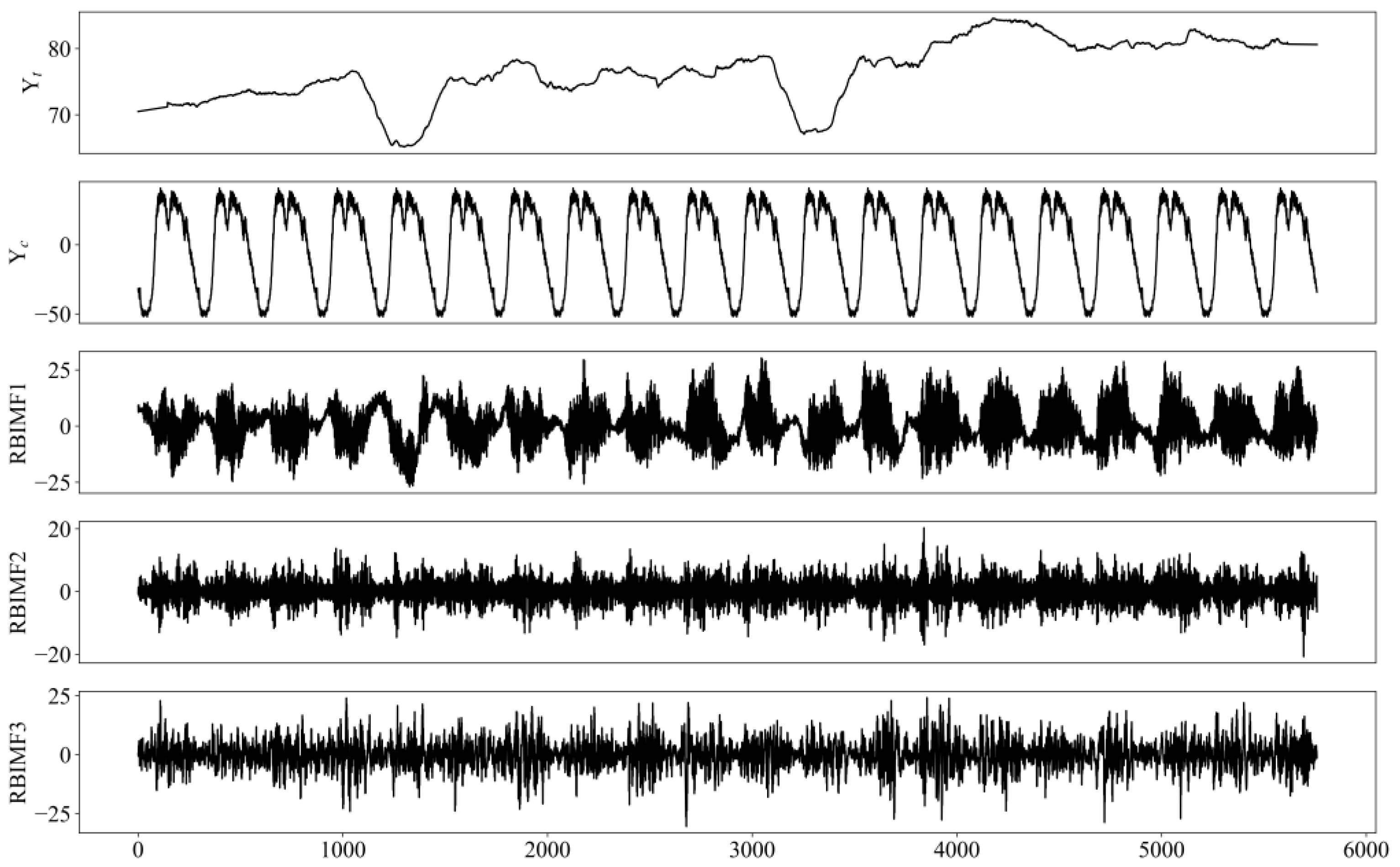The residual term $Y_r$ obtained disorderly changes, but there are still potential features in it, so the optimized VMD is used to decompose $Y_r$ in the second level, and the optimal choice is achieved by the GA of VMD, where =14 and =1880 are obtained, and the decomposition results are shown in Figure 7.

After the secondary decomposition of the traffic flow sequence by STL and VMD, multiple sequence components are obtained. To reduce the complexity of calculation and improve the efficiency of prediction, fuzzy entropy [46] and the Lempel-Ziv [47] complexity index are used to reconstruct the components scientifically and reasonably. Where entropy is a covariate to describe the state of the object to analyze the complexity of the sequence; researchers proposed to use entropy to measure the complexity and fuzzy entropy is to use fuzzy affiliation function instead of Heaviside function in sample entropy so that it can better evaluate the complexity of the sequence more robustly. Unlike the statistical significance of entropy, the Lempel-Ziv complexity index reflects the probability of increasing nonlinear features in the traffic flow, and a larger value indicates that the traffic flow is more complex and contains more nonlinear features.

The components obtained after the second-level decomposition show more obvious and smoother characteristics compared with the original residual terms. To improve the computational efficiency and reduce the interference of subjective factors such as human selection on the prediction effect, the fuzzy entropy (FE) and Lempel-Ziv complexity index (LZ) of each component are calculated for reconstruction, and the calculation results are shown in

Table 3. Fuzzy entropy and Lempel-Ziv complexity index calculation results for BIMFs.

	BIMF1	BIMF2	BIMF3	BIMF4	BIMF5	BIMF6	BIMF7
FE	0.31	0.54	0.57	0.52	0.44	0.35	0.28
LZ	0.10	0.37	0.35	0.37	0.33	0.34	0.25
	BIMF8	BIMF9	BIMF10	BIMF11	BIMF12	BIMF13	BIMF14
FE	0.26	0.30	0.35	0.44	0.52	0.57	0.52
LZ	0.23	0.30	0.35	0.35	0.37	0.38	0.31

.

Referring to FZ first, BIMF (1,7,8,9) is reconstructed to get RBIMF1, BIMF (5,6,10,11) is reconstructed to get RBIMF2, and BIMF (2,3,4,12,13,14) is reconstructed to get RBIMF3. LZ reflects the periodicity of the sequence, and a larger LZ indicates the fewer periodic components inside the sequence; it can be seen from the LZ of each sequence that the LZ of BIMF (1,7,8,9) is smaller, and the periodicity feature is more obvious; the LZ of BIMF (2,3,4,12,13,14) is larger, which indicates that the regularity of sequence change is weaker, which fully proves the rationality of component reconstruction. The results of the trend and period components obtained from the joint STL decomposition of the reconstructed components are shown in Figure 8.

After multiple experiments to determine the time step of the model input, see

Table 4. Inputs and feature combinations for each component.

Portion Size	Input Combinations
$Y_t$	$\left(x_{t-1},x_{t-2},x_{t-3},x_{t-4},x_{t-5},x_{t-6},x_{t-7}\right)$
$Y_c$	$\left(x_{t-1},x_{t-2},x_{t-3},x_{t-4},x_{t-5},x_{t-6},x_{t-7},x_{t-8}\right)$
$\mathrm{RBIMF}1$	$\left(x_{t-1},x_{t-2},x_{t-3},x_{t-4},x_{t-5},x_{t-6},x_{t-7},x_{t-8},T_1\right)$
$\mathrm{RBIMF}2$	$\left(x_{t-1},x_{t-2},x_{t-3},x_{t-4},x_{t-5},x_{t-6},x_{t-7},x_{t-8},x_{t-9},T_2\right)$
$\mathrm{RBIMF}3$	$\left(x_{t-1},x_{t-2},x_{t-3},x_{t-4},x_{t-5},x_{t-6},x_{t-7},x_{t-8},T_3\right)$

, the reconstructed components are combined with the feature set $T$ and input into the model for prediction. The selection of feature sets $T$ is related to the input dimension of each component; RBIMF1 has the feature set $\left[{\mathrm{H}}_{(t-1)~(t-8)}{,\mathrm{J}}_{(t-1)~(t-8)},\cdots {,\mathrm{d}}_{2,(t-1)~(t-8)}{,\mathrm{d}}_{3,(t-1)~(t-8)}\right]$ with 136 features, RBIMF1 has 153 features, and RBIMF1 has 136 features.

To improve the training efficiency of the model, principal component analysis (PCA) is used to extract the main components in the feature set, and as shown in

Table 5. PCA dimensionality reduction analysis.

Feature Set	Ingredient Selection	Cumulative Contribution Rate
$T_1$	1~10	93.05%
$T_2$	1~11	93.12%
$T_3$	1~10	93.05%

, the first 10 components are selected for $T_1$ and $T_3$, and the first 11 components are selected for $T_2$, which can ensure the prediction effect of the model and also save computational resources significantly.

4.4. Evaluation Criteria

To evaluate the prediction effect of the model, the root mean square error ($E_{RMSE}$) and the mean absolute error ($E_{MAE}$) are selected as evaluation indicators, and the smaller the value, the higher the prediction accuracy of the model.

$$E_{RMSE}=\sqrt{\frac{1}{n}{{\displaystyle \sum _{i=1}^n\left(x_i-x_i\right)}}^2}$$

(15)

$$E_{MAE}=\frac{1}{n}\sum _{i=1}^n\left|\left(x_i-x_i\right)\right|$$

(16)

where $n$ is the sample size, $x_i$ is the actual value, and $x_i$ is the predicted value.

4.5. Model Parameter Setting

The parameter settings have a significant impact on the prediction effect of the model. For the KELM model, GA is used to optimize the regularization parameter $c$ and the kernel parameter $\sigma$ in it, and the Gaussian kernel function with better generalization ability is selected for the kernel function. For the LightGBM model, the Bayesian Optimization method is used to optimize the maximum depth of the tree in the model ($max\_depth$), the leaf tree of each tree ($num\_leaves$), and the learning rate ($learning\_rate$). The parameters of LSTM that affect its prediction effect are mainly the number of hidden layer neurons $n$. The parameters are determined by experimental comparison.

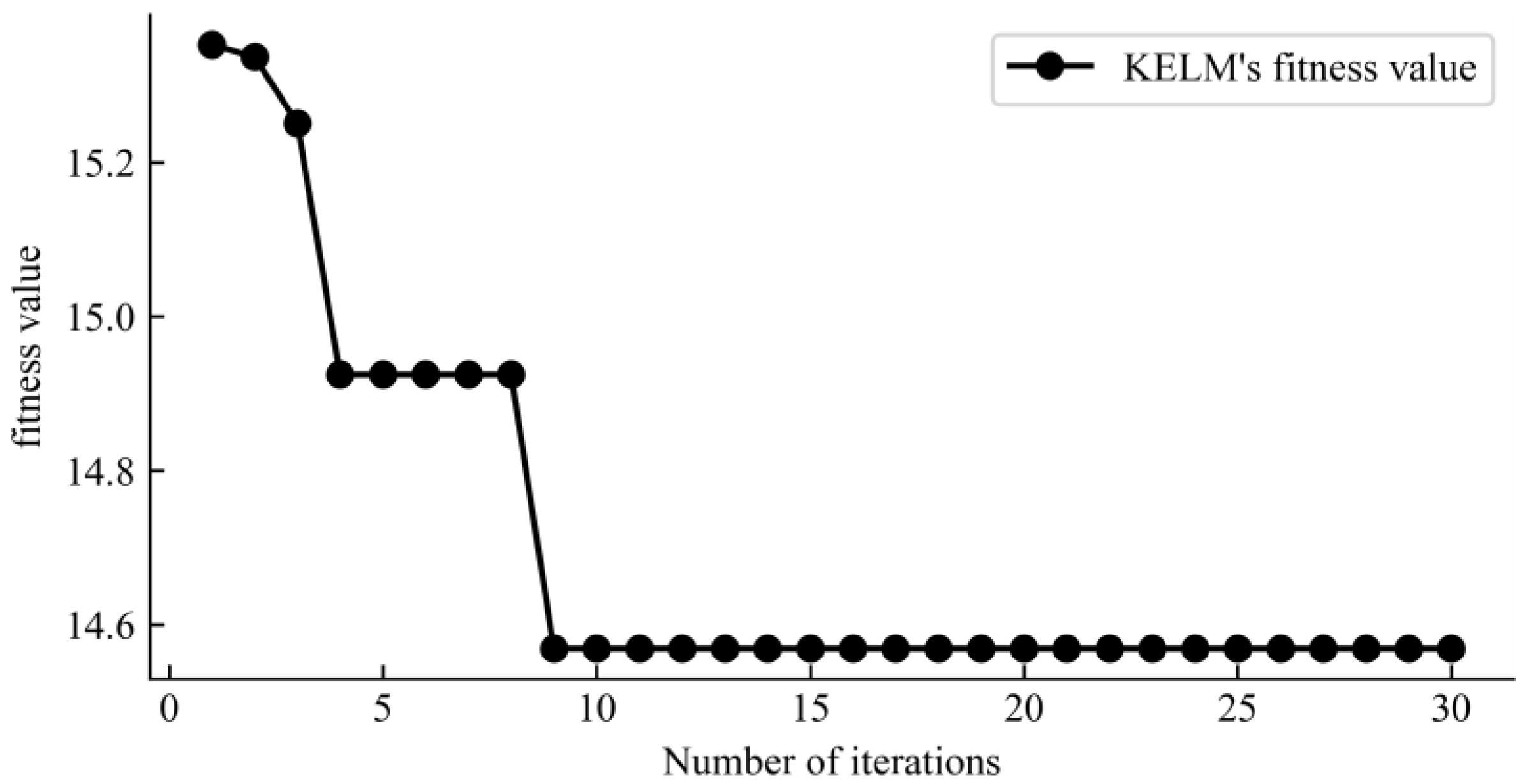
The component RBIMF1 is used as an example for parameter setting, where GA-KELM uses the error as the fitness function to obtain the optimal $\left[c,\sigma \right]$ combination, and the fitness curve is shown in Figure 9, which reaches the optimum at the 9th iteration when $c$ = 74.238 and $\sigma$ = 1.961. 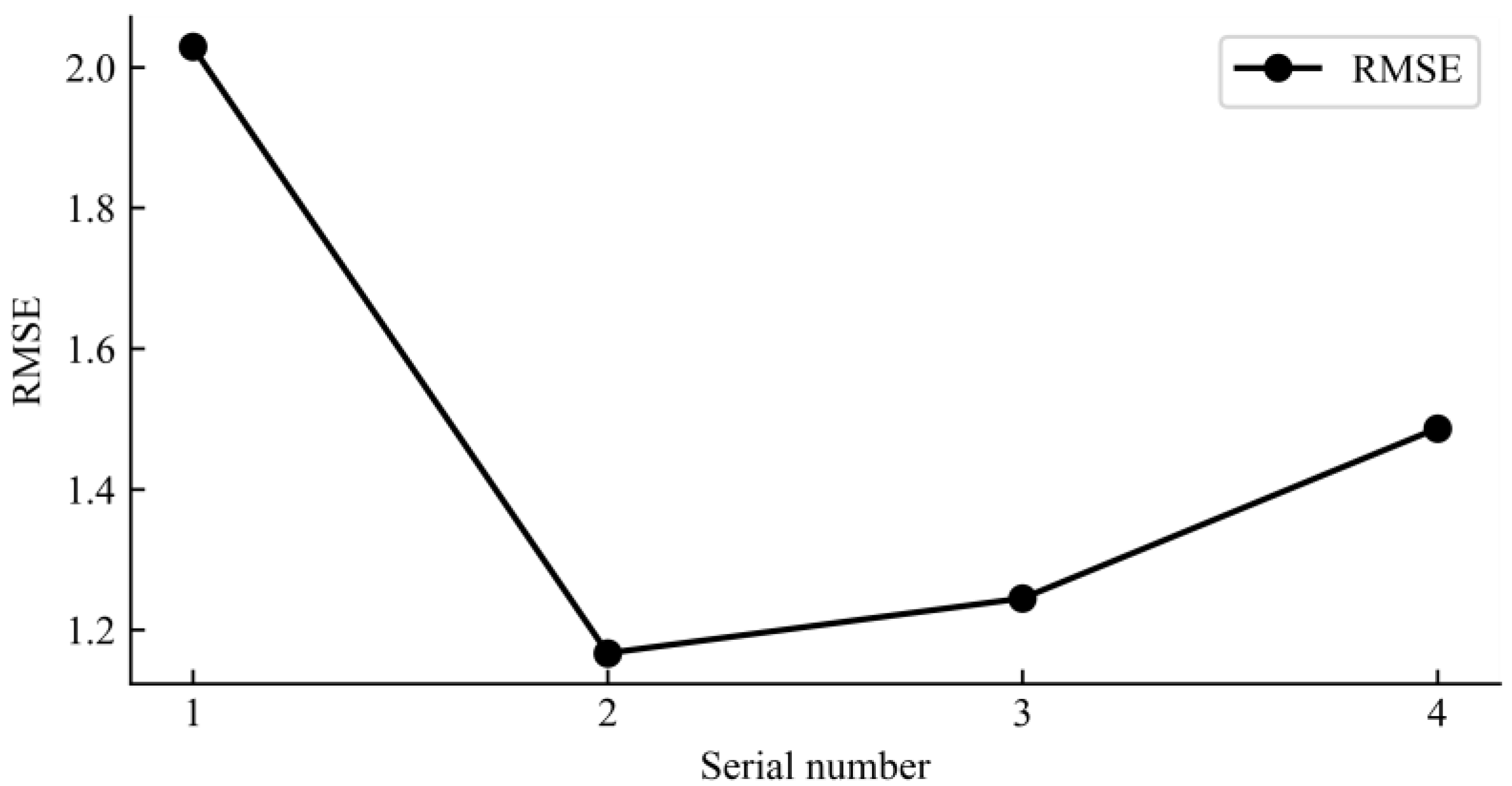LightGBM uses $R^2$ fitting goodness as the search criterion to obtain the optimal combination of parameters, $max\_depth$ = 2, $num\_leaves$ = 165, and $learning\_rate$ = 0.136; LA’s parameters $n$ are taken as 16, 32, 64, and 128, a total of four combinations, and the learning rate $lr$ = 0.01. The prediction error of different parameters of LA is shown in Figure 10, and the prediction error is minimized when $n$ = 32.

4.6. Discussion

4.6.1. Ablation Experiments and Analysis

To verify the effectiveness of each module, the following models are established: a reinforcement learning combined prediction model considering multiple factors (T-Q (E_L_LA)), a reinforcement learning combined prediction model with second-level decomposition (D-Q (E_L_LA)), a combined prediction model with second-level decomposition considering multiple factors with equal weights (D-T-E (E_L_LA)), and the prediction effects of the above models are compared with the model in this paper (D-T-Q (E_L_LA)).

From the error analysis in Figure 11, it can be seen that the decomposition module in the model plays an important role in the prediction of complex traffic flow, which can effectively reduce the unsteadiness of traffic flow. Before and after decomposition, $E_{RMSE}$ is reduced by 71.39% and $E_{MAE}$ is reduced by 71.67%; when the interference of external factors on traffic flow is considered, $E_{RMSE}$ is reduced by 10.61% and $E_{MAE}$ is reduced by 9.56%, indicating that fully considering external factors can improve. For the model weight assignment, compared with the equal weight assignment, the Q-learning assignment reduces the model error $E_{RMSE}$ by 3.74% and $E_{MAE}$ by 3.35%, which improves the prediction accuracy.

4.6.2. Comparison and Analysis of Prediction Results of Different Models

To verify the prediction effectiveness of the models, the following models were built for comparative analysis: LSTM, a combined model of convolutional neural network and gated recurrent unit (CNN-GRU), prediction of the components obtained from the two-stage decomposition using the GA-optimized BP (D-GA-BP), and prediction of the components obtained from the two-stage decomposition using LightGBM (D-LightGBM).

In Figure 12a–e, it can be seen that the prediction curve of the D-T-Q (E-L-LA) model proposed in this paper matches the actual traffic flow curve the best, while the prediction curve of the LSTM model without using the second-level decomposition only roughly predicts the trend of the actual traffic flow curve without capturing the features at the inflection point; the CNN-GRU uses spatio-temporal data for prediction, and its prediction effect is better than the prediction effect of CNN-GRU using spatio-temporal data, which is better than that of LSTM. After introducing spatio-temporal features, the model can extract more information, which is more beneficial to the model prediction.

From

Table 6. Prediction errors across models.

Model	${\mathit{E}}_{\mathit{M}\mathit{A}\mathit{E}}$	${\mathit{E}}_{\mathit{R}\mathit{M}\mathit{S}\mathit{E}}$
LSTM	9.561	12.459
CNN-GRU	7.923	10.242
D-GA-BP	5.232	6.705
D-LightGBM	2.883	3.913
D-T-Q (E-L-LA)	2.622	3.479

, it can be seen that D-T-Q (E_L_LA) reduces $E_{MAE}$ by 72.58% and $E_{RMSE}$ by 72.08% compared with LSTM, $E_{MAE}$ by 66.91% and $E_{RMSE}$ by 66.03% compared with CNN-GRU, $E_{MAE}$ by 49.89%, and $E_{RMSE}$ by 48.11% compared with D-GA-BP, and $E_{MAE}$ by D-LightGBM $E_{MAE}$ reduced by 9.05% and $E_{RMSE}$ reduced by 11.09%. From the comparison of the prediction effect and error of each model, it can be seen that D-T-Q (E_L_LA) has the smallest prediction error and can effectively reduce the unsteadiness of traffic flow and fully consider the external factors to fully extract the features in the traffic flow by combining models to improve the prediction accuracy of the model. However, the current study only verified the effectiveness of the model on single-step prediction, but for path planning and congestion formation analysis, multi-step prediction of traffic flow is more necessary.

5. Conclusions

This paper takes road traffic flow in Changsha city as the research object, effectively reduces the nonlinearity of complex traffic flow by the two-stage decomposition method, fuses the external characteristics of traffic flow for prediction, and finally optimizes the weights of the three prediction models established by Q-learning algorithm to obtain the optimal prediction results. Through the comparison and analysis of ablation experiments and other models, the conclusions are as follows:

• Using STL and VMD, two-level decomposition can effectively reduce the unsteadiness of traffic flow data and decompose it into multiple smooth components, i.e., it can fully explore the intrinsic features of traffic flow and also allow the model to better extract the features in it. The impact of each module on the prediction accuracy was analyzed by ablation experiments, in which the decomposition module improved the prediction effect the most.
• It is important to improve the prediction accuracy by fully considering the spatial and temporal correlation of traffic flow and the influence of the external environment on traffic flow.
• Three phase-divergent models, GA-KELM, LightGBM, and LSTM-Attention, are constructed, and the Q-learning method is used to integrate the three single models, which can fully extract the potential features in the traffic flow and fuse the advantages of each model. Compared with other models, the evaluation index of the model D-T-Q (E_L_LA) in this paper is lower and more suitable for the prediction of short-time traffic flow.

In conclusion, the short-time traffic flow prediction method proposed in this paper is feasible and has a good prediction effect for short-time traffic flow.

The current study can be further delved into by the following aspects: First, traffic accidents are also an important factor affecting the traffic status, and when a traffic accident occurs, it will lead to abnormal traffic flow, so using it as an influencing factor can improve the accuracy of the prediction. Second, the performance of the model is only verified in the current single-step prediction, and it is noteworthy that multi-step prediction is also important for ITS. Third, the method in the paper can still be applied to highway scenarios and tasks, such as traffic speed prediction and travel time prediction, which will help improve road access efficiency and safety through the high accuracy prediction results obtained.