Seven-Phase PMSM Drives Operation Post Two Types of Faults

Abstract

This research presents a seven-phase PMSM drive with a high degree of reliability. This enhancement in reliability is achieved by applying two new Fault Tolerant Control techniques (FTC) at the same time. The first FTC will maintain the operation of the seven-phase PMSM drive after the failure in one based on the minimum inverter current optimization technique. The implementation of this FTC technique is achieved through developing a novel Space Vector Pulse Width Modulation (SVPWM) to assure proper distribution of the currents in the remaining phases post failure. The second FTC technique keeps the operation of the faulty seven-phase PMSM drive post the failure in the speed sensor. This is created by developing a new algorithm to obtain the rotor position and speed of the faulty seven-phase PMSM drive based on the voltage excitation method. Simulation results are presented to demonstrate the enhancement in the reliability achieved by the FTCs developed in this paper for the seven-phase motor drive running post the failures in phase ‘A’ and the speed sensor at the same time.

1. Introduction

Multi-phase machines are witnessing an increasing concern in many industrial applications, especially for medium- and high-power applications such as in the marine, aerospace, and railway industries. This interest is related to the fact that the multi-phase machines offer some advantages over the three-phase drives. Firstly, it possible to obtain a higher power rating motor without the need to increase the phase current or the voltage (same IGBT rating). Secondly, it helps to suppress the harmonics in the torque [1,2,3]. Finally, it offers a high degree of reliability as it is inherently fault-tolerant.

The research on multi-phase motor drives has been devoted in three directions: the first one dedicated on the study of the fault-tolerant design of the multi-phase drive [4,5,6,7,8]; the second one concentrated on the modelling of these drives [9,10], and the last one was studying the control of the multi-phase drive [11,12,13].

Among the above areas of research of the multi-phase motor drives, the fault-tolerant feature has received most of the interest in the research. The fault-tolerant control techniques (FTC) can be classified into active and passive. The active technique uses the data obtained by the fault-detection and diagnosis unit to reconfigure the controller post the failure in one of the system components such as (sensors, actuators) [14,15]. The passive FTC depends only on the redundancies of the system and uses only one controller which is robust against the predefined set of failures [16,17]. As a result, the passive FTC is considered much simpler but on the other hand, its robustness is much lower than the active FTC.

The accomplishment of post-fault drive operation requires the suitable choice of references to be applied. The optimal values of reference currents are determined based upon the particular drive arrangement and the type of winding connection. Most of the introduced reference currents calculation procedures were applied offline utilizing the mathematical model of the machine and the required torque production. These techniques can be classified as follows: maximum torque, minimum losses, and minimum torque ripple [18,19,20].

However, to control healthy currents of the multi-phase drive post the fault according to the above techniques, many controller types were used. One of these controllers was the hysteresis current controller [21,22,23]. Although this technique is very easy to implement, it has a variable switching frequency that makes it undesirable in the motor drives. Another control technique was the using Vector Control technique based on using a modified SVPWM technique post the fault [24,25].The Vector Control technique is based on using new transformation matrices can be used to control the new multi-phase currents post the fault [26,27,28,29,30]. In addition to hysteresis and vector control, other control techniques were also used to control the multi-phase motor currents post the fault such as: Direct-Torque Control (DTC) [31], Sliding Mode Control [32], Model predictive control [33].

Another type of fault that has been research in the last couple of years in the multi-phase motor drive was the fault in the speed sensor (i.e., sensorless operation). Many techniques have been suggested to obtain the speed and the position of the multi-phase motor post the fault in the speed sensor including model-based technique, DTC, and voltage and current excitation techniques [34,35,36,37,38]. In the last two years, some papers have proposed a fault-tolerant five-phase motor drive that able to work post the failure in one phase and the failure in the speed sensor [39,40].

This is the first paper that is introducing a fault-tolerant seven-phase drive that has the ability to run post the failures in speed sensor and phase ‘A’ happened at the same time. Firstly, the paper introduces a new SVPWM technique of the seven-phase PMSM drive post the failure in phase ‘A’ to assure proper distribution of the remaining healthy currents according to the maximum torque FTC technique (minimum inverter current technique). Secondly, the paper proposes a new algorithm to obtain the rotor position and speed of the faulty seven-phase PMSM drive to keep its operation post the fault in the speed sensor and in post the failure in phase ‘A’.

2. Operation of the Seven-Phase Drive Post the Speed Sensor Failure

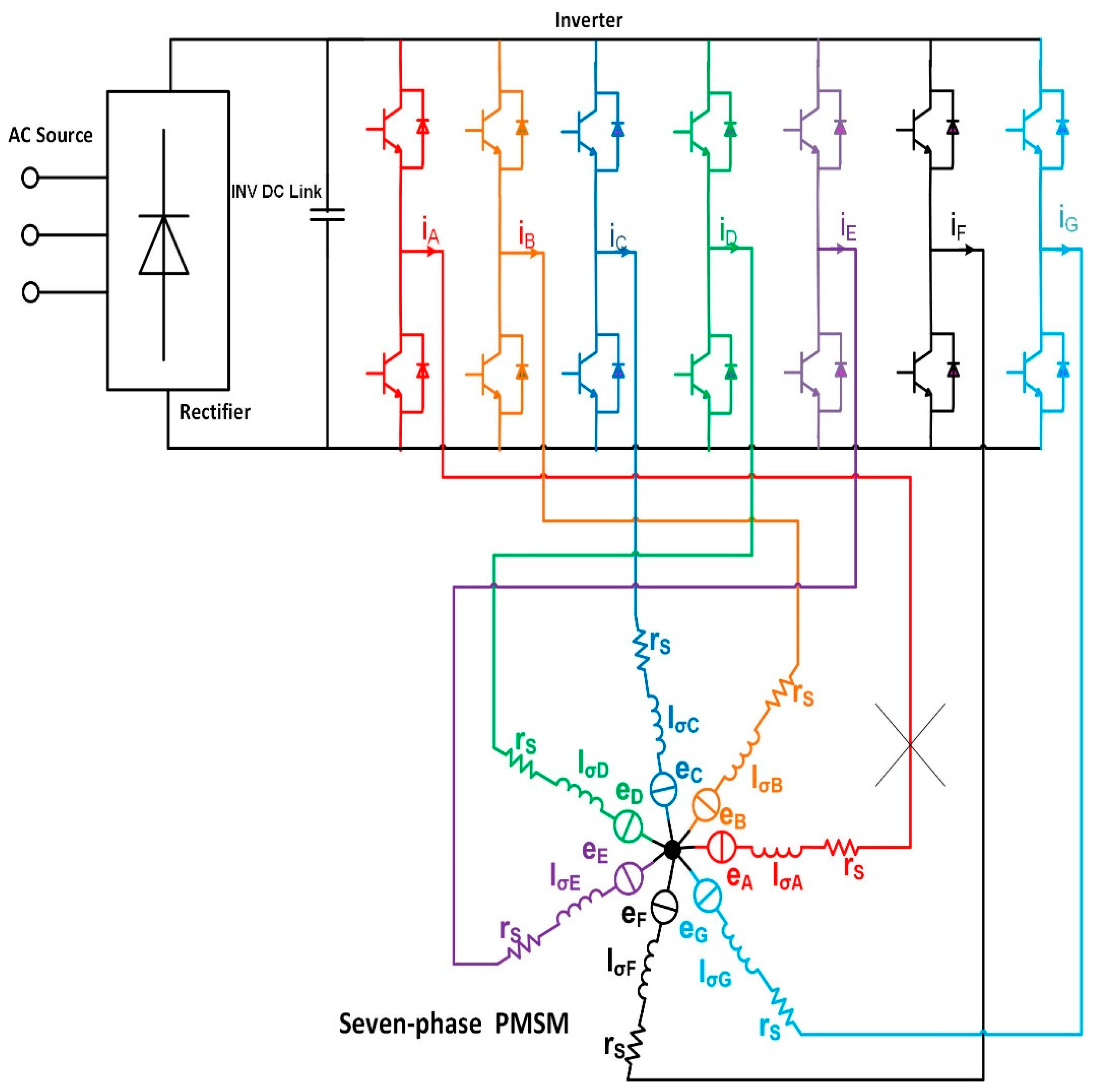
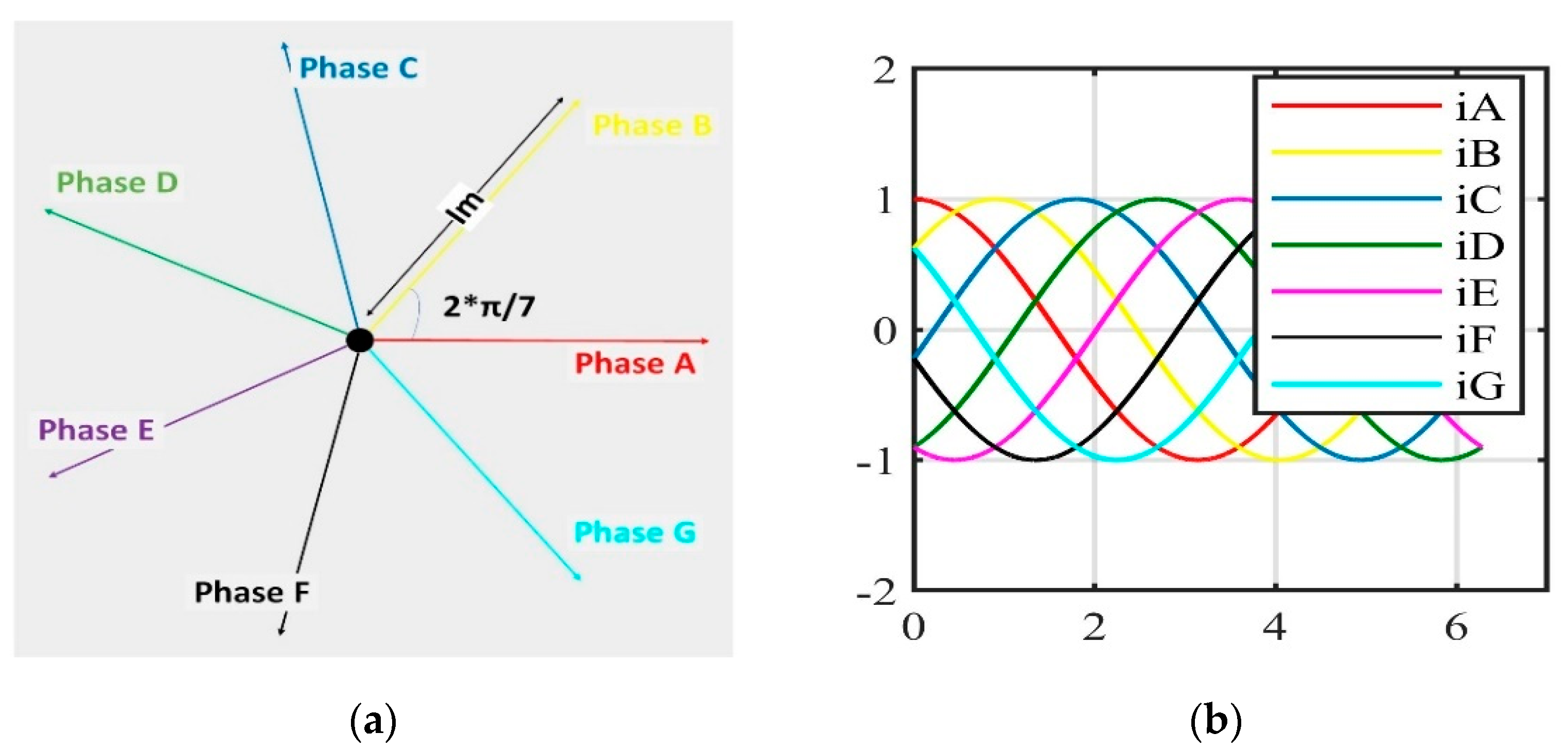
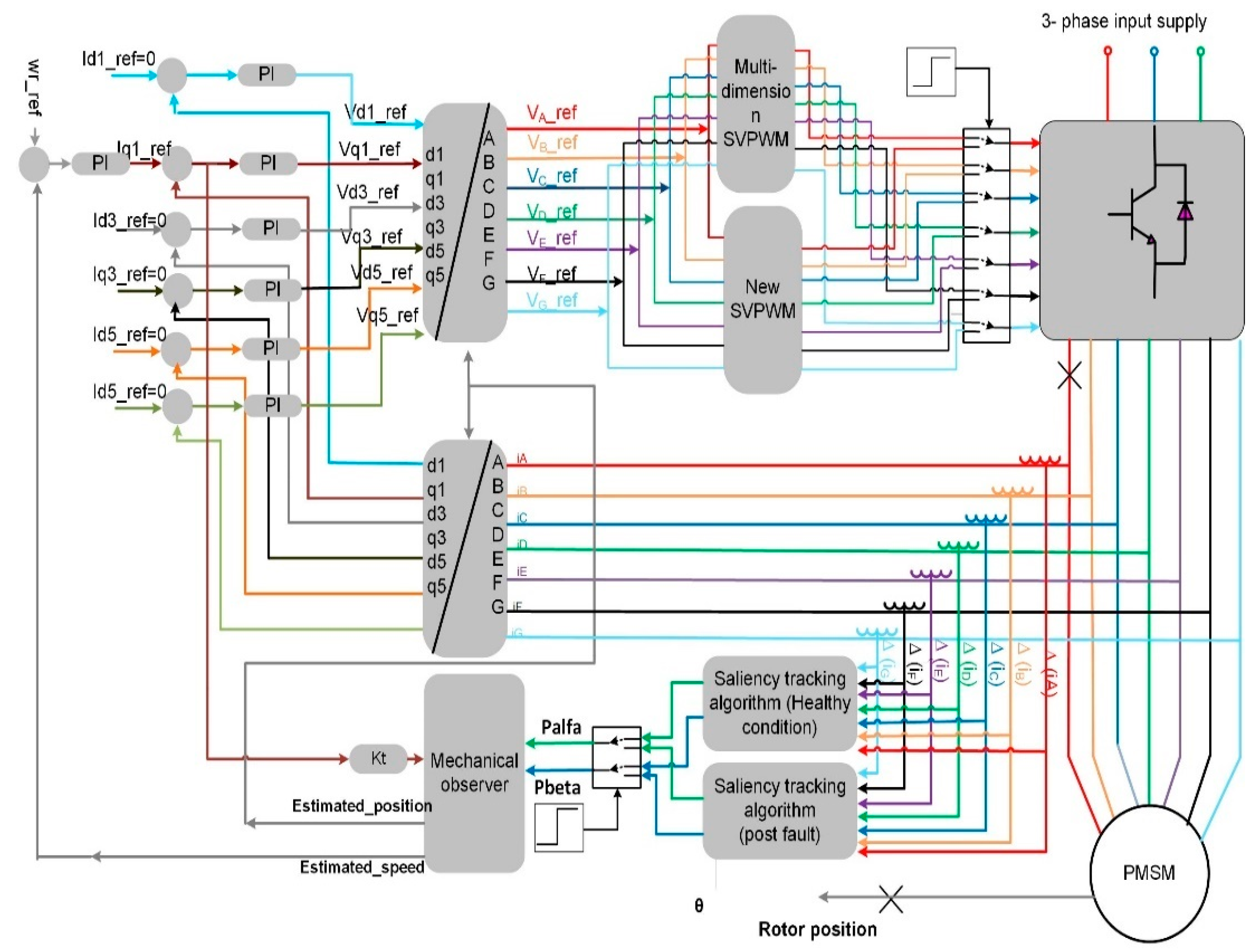
2.1. Seven-Phase PMSM Model

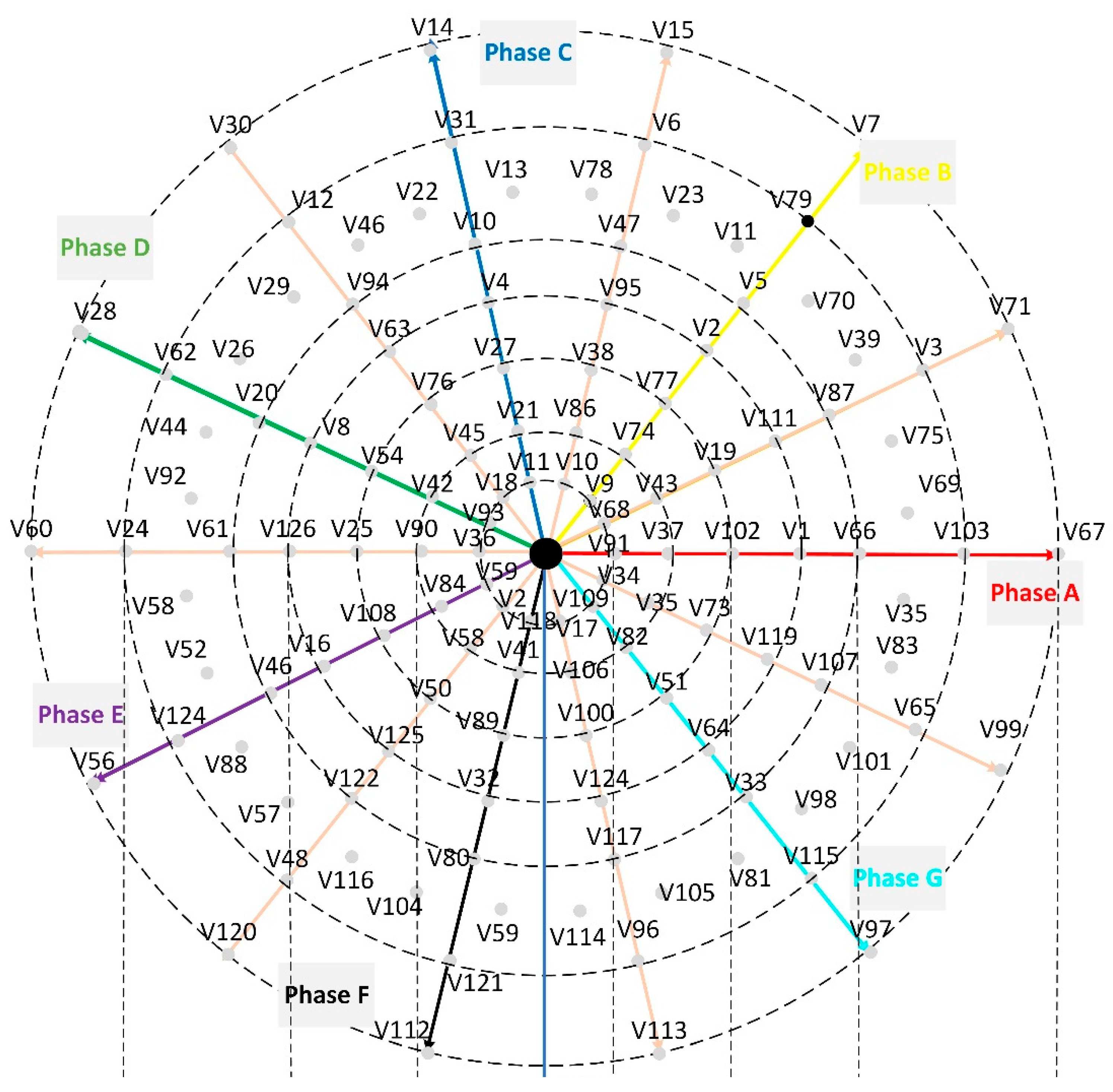
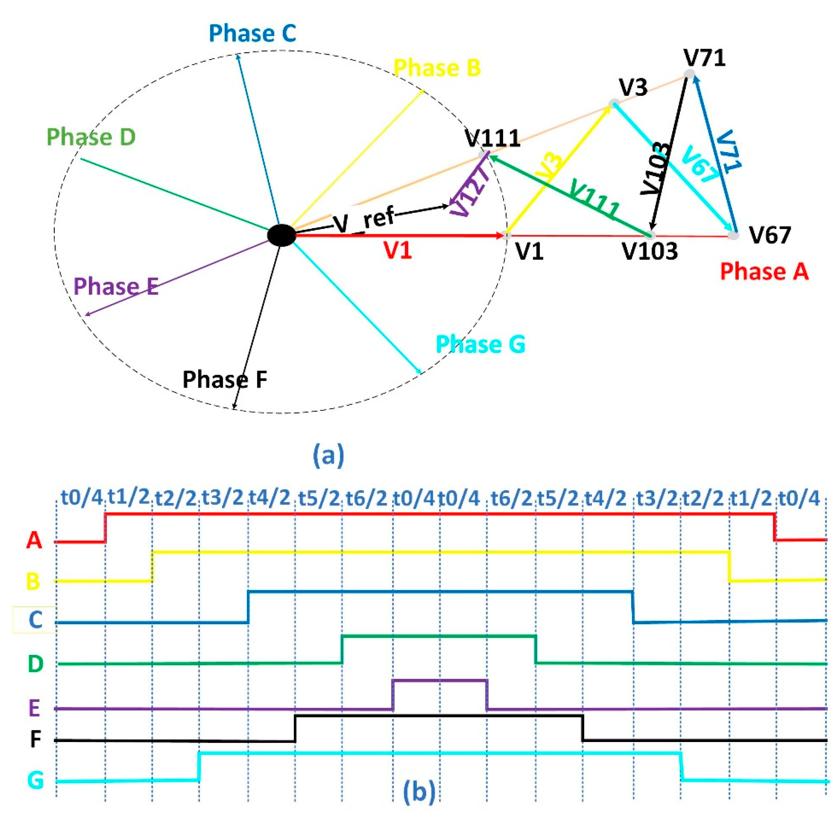
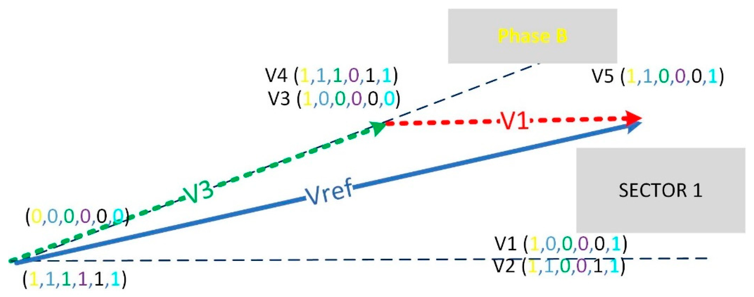
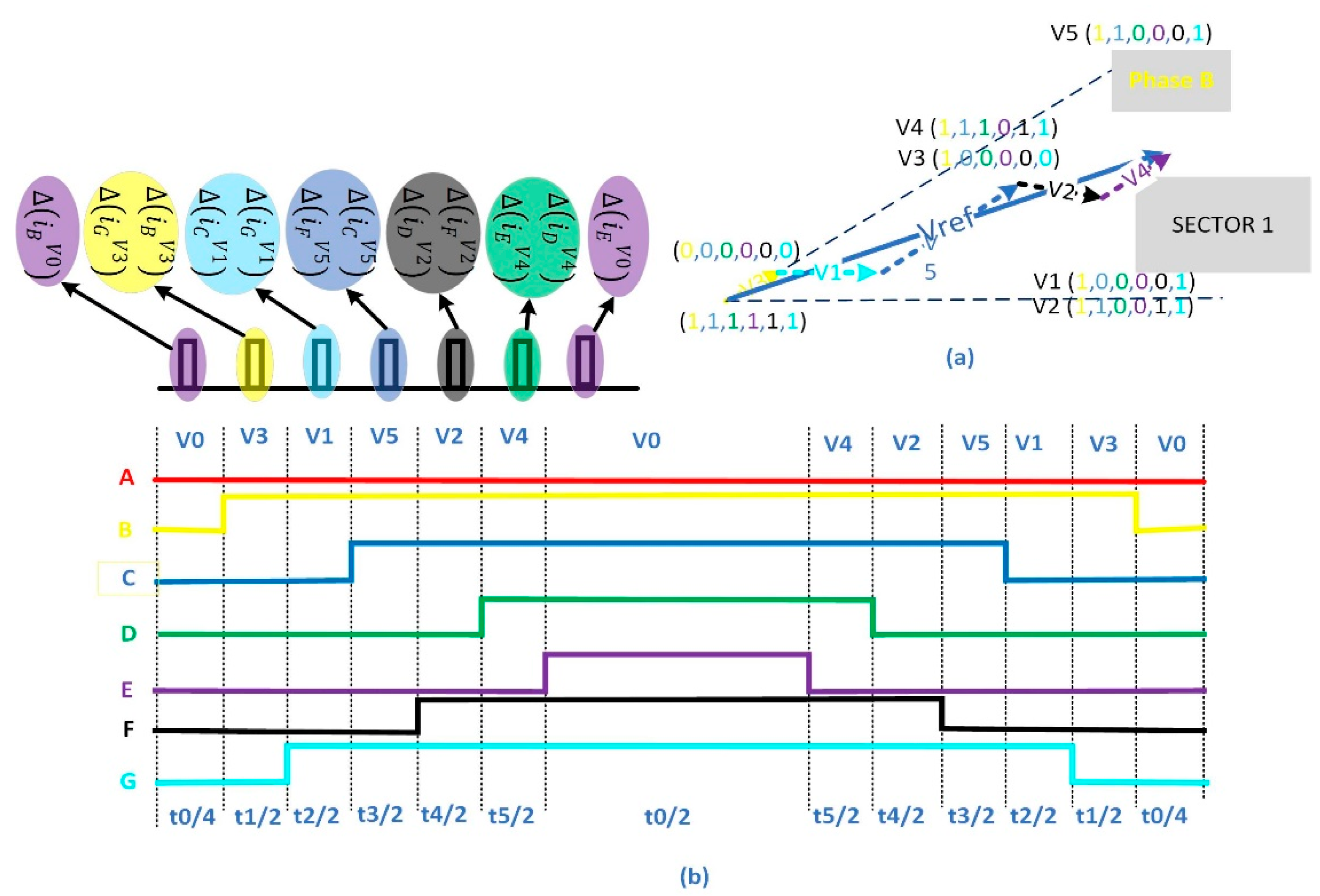
The topology of the seven-phase PMSM drive is depicted in Figure 1. The exact model of the seven-phase PMSM is expressed on the Equations (1)–(3).

$$\left[V_s\right]=r_s\ast \left[I_s\right]+\Delta \left[{\mathsf{\phi }}_s\right]$$

(1)

where $\left[V_s\right]=\left[V_{sA},V_{ sB},V_{sC},V_{sD},V_{sE},V_{sF},V_{sG}\right]{ }^T$ are the inverter output voltages, $\left[I_s\right]=\left[i_{sA},i_{sB},i_{sC},i_{sD},i_{sE},i_{sF},i_{sG}\right]{ }^T$ are the stator currents, $\left[ {\phi }_s\right]=\left[{\phi }_{sA},{\phi }_{ sB},{\phi }_{sC},{\phi }_{sD},{\phi }_{sE},{\phi }_{sF},{\phi }_{sG}\right]{ }^T$ are the stator linkage fluxes, $r_{s }$is the stator resistance, and $\Delta =\frac{d}{dt}$.

The stator linkage fluxes can be expressed as:

$$\left[{\mathsf{\phi }}_s\right]=L_{ms}\ast \left[I_s\right]+{\mathsf{\phi }}_M$$

(2)

$${\mathsf{\phi }}_M={ʎ}_m\ast \left[\begin{array}{c}\begin{array}{c}\cos \left({\theta }_R\right)\\ \cos \left({\theta }_R-2\pi /7\right)\\ \cos \left({\theta }_R-4\pi /7\right)\end{array}\\ \cos \left({\theta }_R-6\pi /7\right)\\ \cos \left({\theta }_R-8\pi /7\right)\\ \cos \left({\theta }_R-10\pi /7\right)\\ \cos \left({\theta }_R-12\pi /7\right)\end{array}\right]$$

(3)

where $L_{ms}$ is the stator inductances matrix, ${ʎ}_m$ is the peak permanent magnet flux linkage, and ${\theta }_R$ is the rotor position. The parameters of the PMSM motor that is used in this paper is given in the Appendix A.

2.2. NSV-SVPWM

The SVPWM that is used in seven-phase drive is called Near Six Vector Space Vector Pulse Width Modulation (NSV-SVPWM) through which the 3rd and 5th harmonics can be suppressed from the output of the inverter. This because these harmonics will generate a huge current in the seven-phase motor as they are limited by the stator impedance only due to the absence of the rotating back EMF [41,42,43]. The space vector distribution that can be generated by switching the even-phase inverter is shown in Figure 2. These vectors can be obtained using the equation:

$$Vs=\frac{2}{7}VDC\left(S_A+S_B{\mathrm{e}}^{j2\pi /7}+S_C{\mathrm{e}}^{j4\pi /7}+S_D{\mathrm{e}}^{j6\pi /7}+S_E{\mathrm{e}}^{j8\pi /7}+S_F{\mathrm{e}}^{j10\pi /7}{}^{}+S_G{\mathrm{e}}^{j12\pi /7}\right)$$

(4)

where $S_A, S_B, S_C, S_D, S_E, S_F$ and $S_G$ are the gating signals of upper switches of the phases ‘A’, ‘B’, ‘C’, ‘D’, ‘E’, ’F’ and ‘G’ respectively in the seven phase inverter.

In each sector, the 6 adjacent active vectors with the length of L4, L5, L6, L7 in addition to the two inactive vectors V0 and V127 are used to synthesize the reference voltages in x1-y1 plane as illustrated in Figure 3a and the associated PWM waveform will be as shown in Figure 3b. The algorithm to implement the NSV-SVPWM can be found in [41,42,43].

2.3. Algorithms to Extract the Rotor Position in Seven-Phase PMSMs

The inductances of the stator winding of the seven-phase PMSM are modulated by the saturation saliency of the main flux. This modulation appears in the derivative of the stator currents of the seven-phase PMSM when any of the IGBTs in the inverter are switched on or off. Hence, the speed and position of the rotor can be extracted by measuring the current derivative due to the IGBTs switching action in one PWM waveform. The technique to extract the rotor position and speed of the seven- phase inverter can be found in [38].

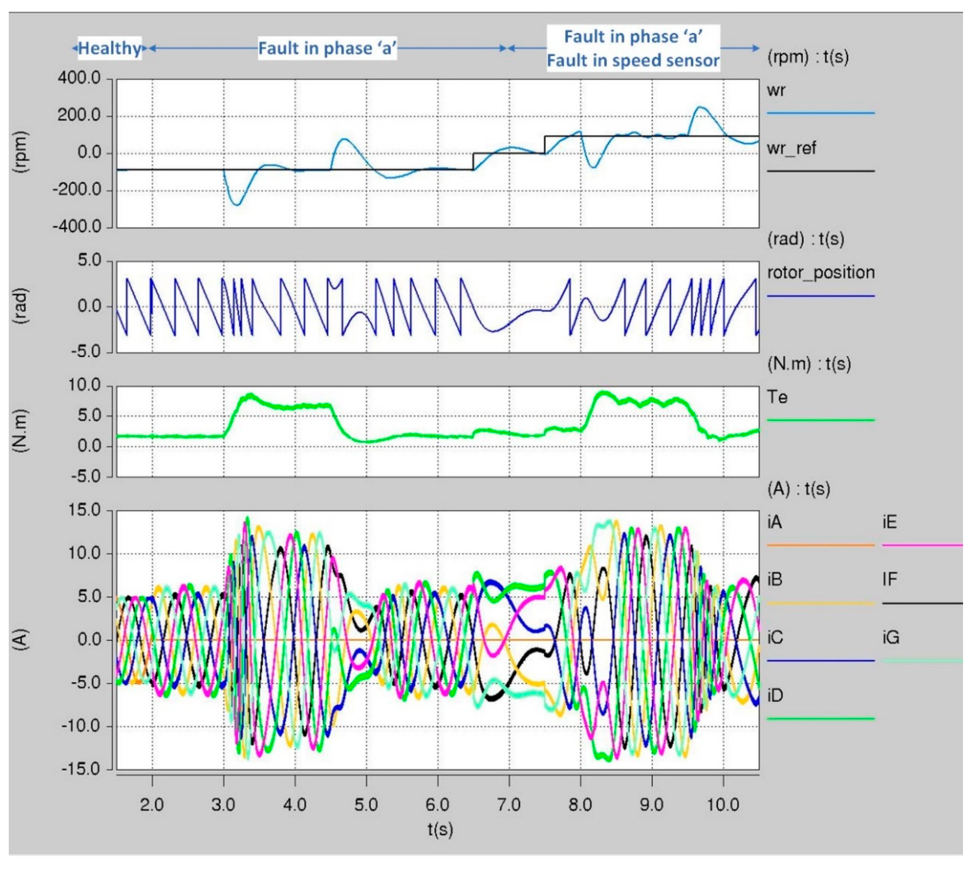
3. Operation of the Seven-Phase Drive after Losing Phase ‘A’

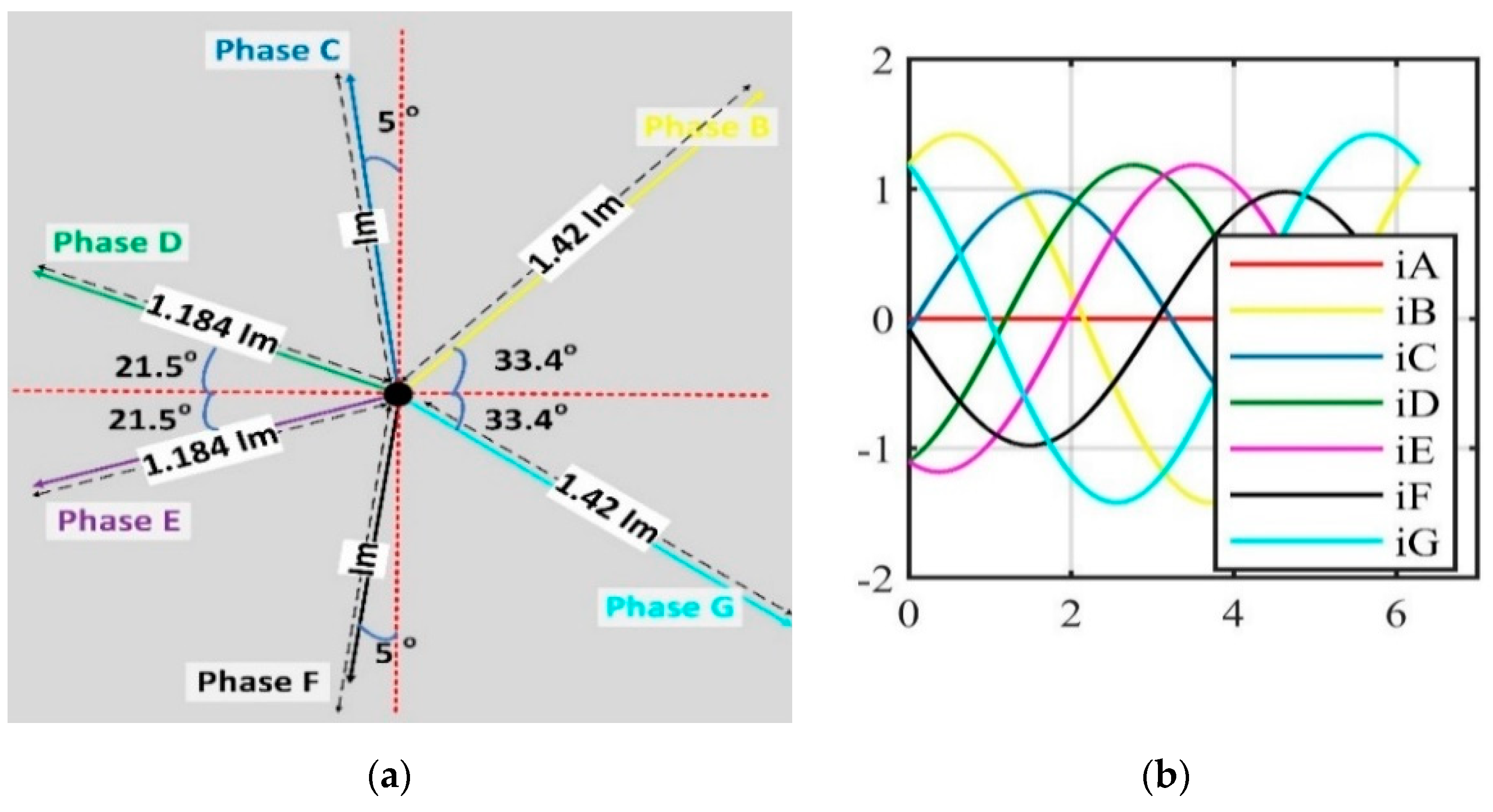
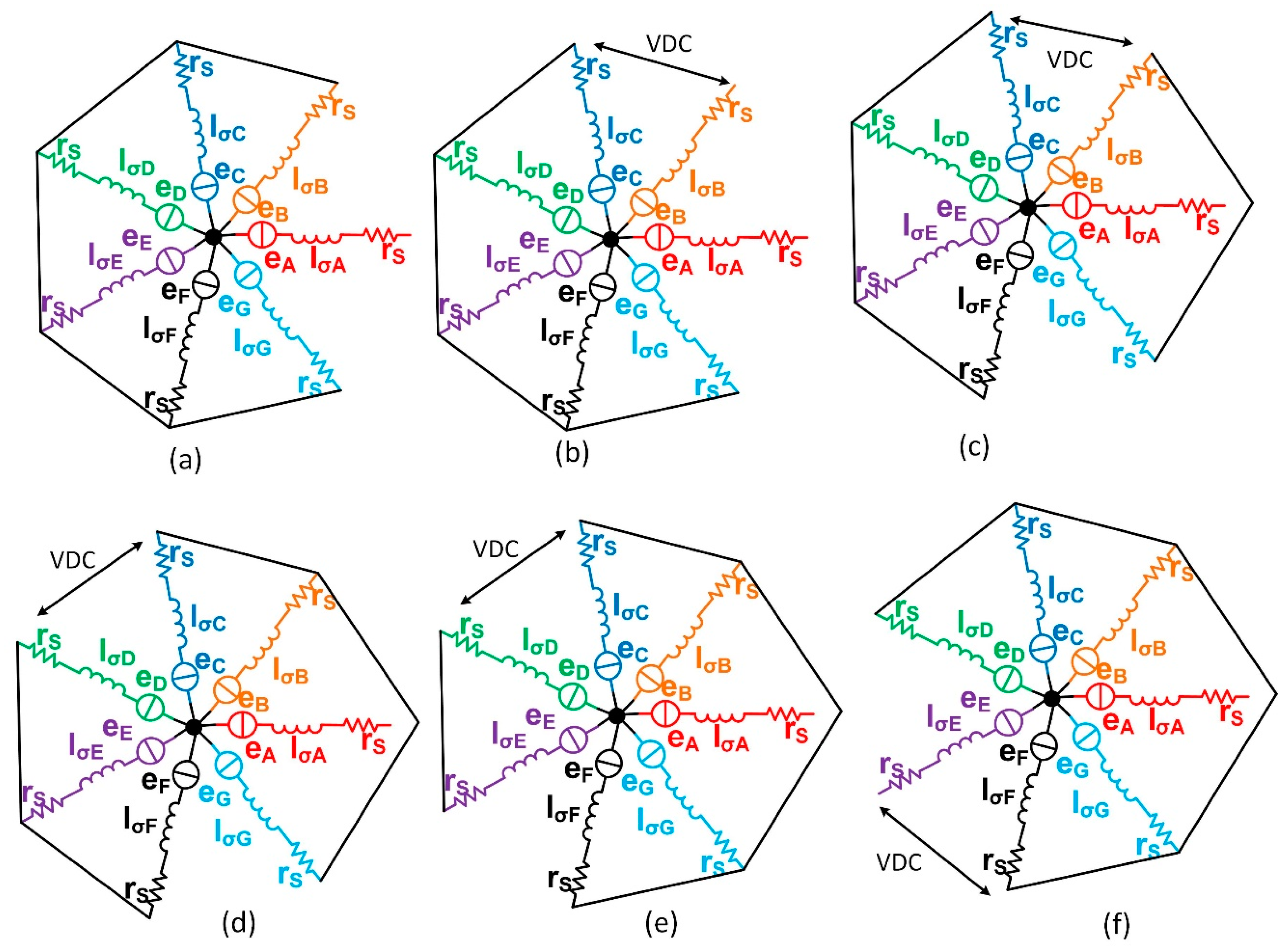
3.1. The Stator Current Distribution in the Seven-Phase PMSMs after Losing Phase ‘A’

When the seven-phase PMSM is running without faults, the currents will be equal in magnitudes and phase shifted by an angle equals $2\pi /7$ as shown in Equation (5) and Figure 4a,b [16,17,18,19,20,44]:

$$\left[\begin{array}{c}\begin{array}{c}{i}_A\\ i_B\\ i_C\end{array}\\ i_D\\ i_E\\ i_F\\ i_G\end{array}\right]=\left[\begin{array}{c}\begin{array}{c}{I}_m\ast \cos \left(wt\right)\\ I_m\ast \cos \left(wt-2\pi /7\right)\\ I_m\ast \cos \left(wt-4\pi /7\right)\end{array}\\ I_m\ast \cos \left(wt-6\pi /7\right)\\ I_m\ast \cos \left(wt-8\pi /7\right)\\ I_m\ast \cos \left(wt-10\pi /7\right)\\ I_m\ast \cos \left(wt-12\pi /7\right)\end{array}\right]$$

(5)

where I_m is the peak value of the phase current.

As mentioned in the introduction, one major advantage of the seven-phase motor drive is that it is inherently fault-tolerant. This means that if one phase is lost due to the open-circuit fault in the seven-phase motor, the motor will be capable to keep on its operation with good dynamic and steady-state performance using a proper FTC technique. The FTC target is to maintain the MMF post the fault pure sinusoidal without harmonics. This can be completed by controlling the healthy currents of the seven-phase motor post the fault according to new predefined reference currents. These new predefined reference currents can be optimized to achieve other goals besides maintaining the MMF. Such as: equalizing current amplitudes after fault, minimizing copper losses, and maximizing torque/power under a given current limit [16,17,18,19,20,44].

According to that, if phase ‘A’ is lost due to the open-circuit fault, the stator reference currents should be modified according to Equation (6) and Figure 5a,b to maintain the MMF and at the same time minimizing the torque ripple [16,17,18,19,20,44].

$$\left[\begin{array}{c}\begin{array}{c}{i}_A\\ i_B\\ i_C\end{array}\\ i_D\\ i_E\\ i_F\\ i_G\end{array}\right]=\left[\begin{array}{c}\begin{array}{c}0\\ 1.585 I_m\ast \cos \left(wt-41.6 °\right)\\ 1.152 I_m\ast \cos \left(wt-94.4 °\right)\end{array}\\ 1.188 I_m\ast cos\left(wt-202°\right)\\ 1.188 I_m\ast \cos \left(wt-158 °\right)\\ 1.152 I_m\ast \cos \left(wt-265.8 °\right)\\ 1.585 I_m\ast \cos \left(wt-318.4 °\right)\end{array}\right]$$

(6)

To maintain the MMF and at the same time minimize the copper losses in the seven-phase motor drive when phase ‘A’ is lost, the stator reference currents should be modified according to Equation (7) and Figure 6a,b [16,17,18,19,20,44].

$$\left[\begin{array}{c}\begin{array}{c}{i}_A\\ i_B\\ i_C\end{array}\\ i_D\\ i_E\\ i_F\\ i_G\end{array}\right]=\left[\begin{array}{c}\begin{array}{c}0\\ 1.42 I_m\ast \cos \left(wt-33.4°\right)\\ I_m\ast \cos \left(wt-95°\right)\end{array}\\ 1.184 I_m\ast \cos \left(wt-158.5°\right)\\ 1.184 I_m\ast \cos \left(wt-201.5°\right)\\ I_m\ast \cos \left(wt-265°\right)\\ 1.42 I_m\ast \cos \left(wt-326.6°\right)\end{array}\right]$$

(7)

Finally, if phase ‘A’ is lost due to an open-circuit fault, the stator reference currents should be modified according to Equation (8) and Figure 7a,b to maintain the MMF and at the same time minimize the inverter current [16,17,18,19,20,44].

$$\left[\begin{array}{c}\begin{array}{c}{i}_A\\ i_B\\ i_C\end{array}\\ i_D\\ i_E\\ i_F\\ i_G\end{array}\right]=\left[\begin{array}{c}\begin{array}{c}0\\ 1.23 I_m\ast \cos \left(wt-21.4 °\right)\\ 1.23 I_m\ast \cos \left(wt-90 °\right)\end{array}\\ 1.23 I_m\ast \cos \left(wt-158.6°\right)\\ 1.23 I_m\ast \cos \left(wt-201.4 °\right)\\ 1.23 I_m\ast \cos \left(wt-270 °\right)\\ 1.23 I_m\ast \cos \left(wt-338.6 °\right)\end{array}\right]$$

(8)

It can be noticed from the results in Figure 7 that the current in the remaining phases after losing phase ’A’ are equal in magnitude based on the minimizing of the inverter current optimization technique. In this paper, the minimizing inverter current optimization technique will be considered only.

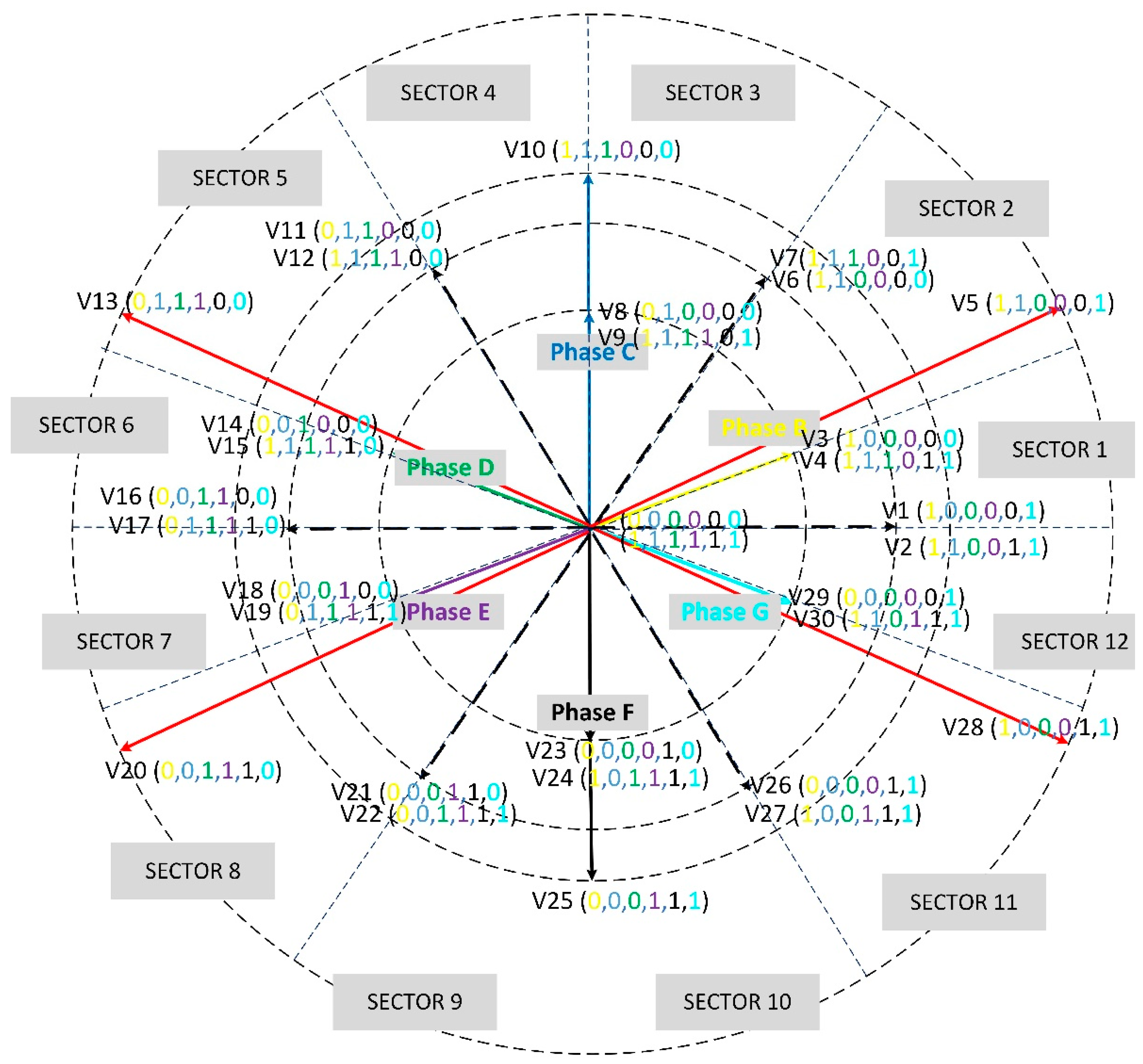
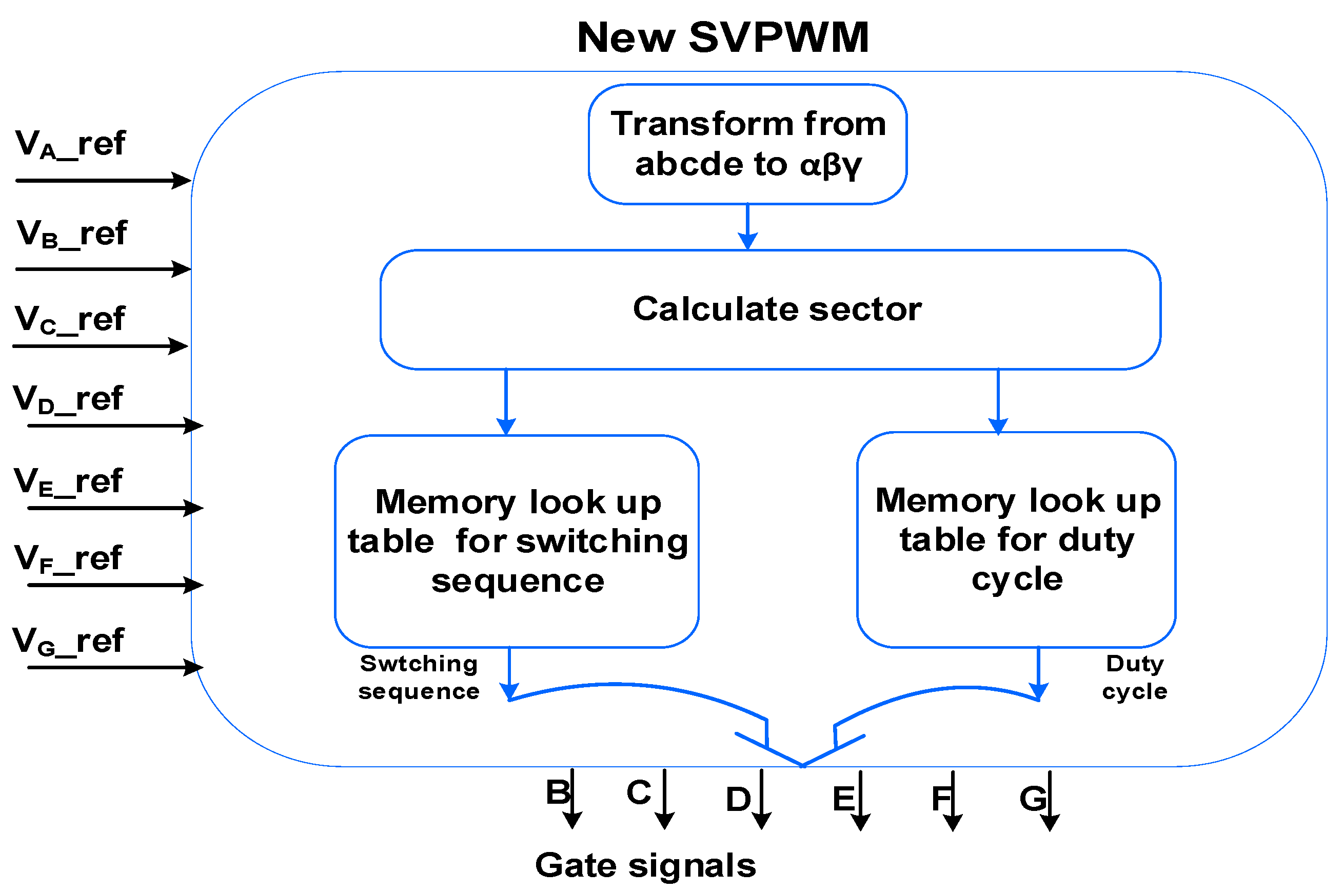
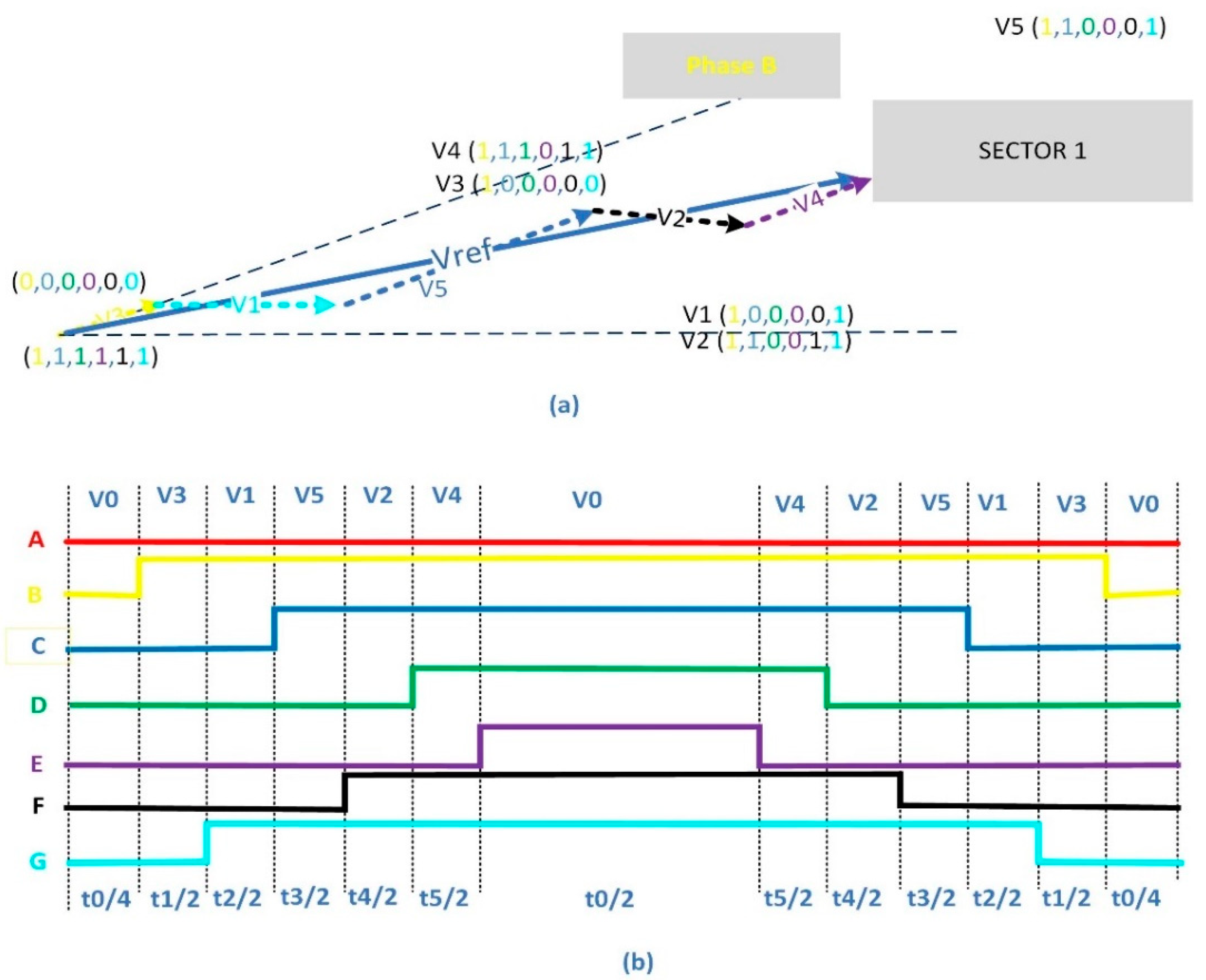
3.2. SVPWM Techniques after Losing Phase ‘A’

The NSV-SVPWM technique that is used in the seven-phase inverter under healthy conditions cannot be applied post the failure, because, the reference currents post the failure will not be uniformly distributed according to the minimizing the inverter current optimization technique as shown in Figure 7. This paper is introducing a new SVPWM technique that will be utilized after the loss of phase ‘A’ to obtain the stator current based on the minimum inverter current optimization technique as illustrated in Equation (8) and Figure 7. The new SVPWM is considering the changes that are introduced to the healthy currents of the seven-phase drive when phase ‘A’ is lost. Hence a new vector diagram is considered as depicted in Figure 8. The new vectors are calculated by putting $S_A=0$ in Equation (4). It should be mentioned here that the new space vector diagram contains 64 vectors, but only the vector that is used to synthesize the reference voltage is considered in Figure 8.

The amplitude of the vectors whose arrows lies on the inner circle will be 0.2857* VDC, the amplitude of the vectors whose arrows lies on the next circle will be 0.4721*VDC, the amplitude of the vectors whose arrows lies on the third circle will be 0.4942*VDC. Finally, the vectors whose arrows lies one the outer circle will be 0.6039*VDC. It should be mentioned here that the vectors V5, V13, V20, and V28 (outer circle) are very close in direction to phase ‘B’, ’D’, ’E’, and ‘G’ respectively as the difference in angles between them is just 6.8⁰ and hence, they will be approximated to be in the same direction in this paper (i.e., the direction of the phases ‘B’, ‘D’, ’E’, and ‘G’).

The flowchart to implement the new SVPWM after losing phase ‘A’ in the seven-phase drive is depicted in Figure 9. The illustration of each part of the flow chart is given below.

Firstly, outputs of the controllers (V_ref) are used to determine the sector no based on

Table 1. Identifying the sector.

Angle of Reference Voltage (θ)	Sector	Angle of Reference Voltage (θ)	Sector
$0°\le \theta <21.4$°	1	$180°\le \theta <201.4°$	7
$21.4°\le \theta <55.7$°	2	$201.4°\le \theta <235.7°$	8
$55.7°\le \theta <90$°	3	$235.7°\le \theta <270°$	9
$90°\le \theta <124.3°$	4	$270°\le \theta <304.3$°	10
$124.3°\le \theta <158.6°$	5	$304.3°\le \theta <338.6$°	11
$158.6°\le \theta <180$°	6	$338.6°\le \theta <360°$	12

.

Secondly, the time duration of each active vector is calculated. Figure 10a illustrates how the adjacent active vectors (V1, V2, V3, V4, V5) besides the null vectors are used to synthesize the V_ref when it exists in the first sector. While Figure 10b shows the PWM waveform associated with applying these vectors.

The application time of the active vectors V1, V2, V3, V4, V5 and V0 i.e., (t0, t1, t3, t3, t4, and t5) can be deduced based on the assumption that the vectors V3, V5, and V4 are in the same direction while the vectors V1, V2 are in the same direction too. Hence, only, two vectors V3 and V1 can be used to calculate the total time duration in the direction of V3,V4, and V5 (i.e., tx), and the total time duration of the vectors V1, and V2 (i.e., ty) as shown in Figure 11. So, after calculating tx and ty, the vector duration times t0, t1, t3, t3, t4, and t5 are obtained considering the length of the vectors as shown in the equations below:

$$\left[\begin{array}{c}V{\alpha }_{ref}\\ V{\beta }_{ref}\end{array}\right]\ast \frac{T}{VDC}=\left[\begin{array}{cc}0.2857\ast \cos \left(21.4°\right)& 0.4721\ast \cos \left(0\right)\\ 0.2857\ast \sin \left(21.4°\right)& 0.4721\ast \sin \left(0\right)\end{array}\right]\ast \left[\begin{array}{c}tx\\ ty\end{array}\right]$$

(9)

where $V{\alpha }_{ref}, V{\beta }_{ref}$ are the component of V_ref in the $\alpha \beta$ T is the PWM period.

Solving the above equation yields to:

$$\left[\begin{array}{c}tx\\ ty\end{array}\right]=\frac{T}{VDC}\left[\begin{array}{cc}0& 7.41\\ 2.13& -3.954\end{array}\right]\ast \left[\begin{array}{c}V{\alpha }_{ref}\\ V{\beta }_{ref}\end{array}\right]$$

(10)

$$to=T-tx-ty$$

(11)

Then vector duration times t1, t2, t3, t4, and t5 can be calculated according to the length of the vectors V1, V2, V3, V4, and V5 as follows:

$$\left[\begin{array}{c}t1\\ \begin{array}{c}t2\\ \begin{array}{c}t3\\ \begin{array}{c}t4\\ t5\end{array}\end{array}\end{array}\end{array}\right]=\left[\begin{array}{c}0.25\ast tx\\ \begin{array}{c}0.5\ast ty\\ \begin{array}{c}0.5\ast tx\\ \begin{array}{c}0.5\ast ty\\ 0.25\ast tx\end{array}\end{array}\end{array}\end{array}\right]$$

(12)

The dwell time and the switching sequence in each sector associated with applying the new SVPWM can be found in

Table 2. Dwell time calculation and switching sequence of the active vectors in the new SVPWM.

Sector	Switching Time	Switching Sequence
1	$\left[\begin{array}{c}tx\\ ty\end{array}\right]=\frac{T}{VDC}\left[\begin{array}{cc}0& 9.6\\ 2.13& -5.42\end{array}\right]\ast \left[\begin{array}{c}V{\alpha }_{ref}\\ V{\beta }_{ref}\end{array}\right]$	V3, V1, V5, V2, V4
2	$\left[\begin{array}{c}tx\\ ty\end{array}\right]=\frac{T}{VDC}\left[\begin{array}{cc}5.13& -3.5\\ -1.37& 3.5\end{array}\right]\ast \left[\begin{array}{c}V{\alpha }_{ref}\\ V{\beta }_{ref}\end{array}\right]$	V3, V6, V5, V7, V4
3	$\left[\begin{array}{c}tx\\ ty\end{array}\right]=\frac{T}{VDC}\left[\begin{array}{cc}-5.13& 3.5\\ 3.7& -0.0011\end{array}\right]\ast \left[\begin{array}{c}V{\alpha }_{ref}\\ V{\beta }_{ref}\end{array}\right]$	V8, V6, V10, V7, V9
4	$\left[\begin{array}{c}tx\\ ty\end{array}\right]=\frac{T}{VDC}\left[\begin{array}{cc}5.13& 3.5\\ -3.76& 0.0011\end{array}\right]\ast \left[\begin{array}{c}V{\alpha }_{ref}\\ V{\beta }_{ref}\end{array}\right]$	V8, V11, V10, V12, V9
5	$\left[\begin{array}{c}tx\\ ty\end{array}\right]=\frac{T}{VDC}\left[\begin{array}{cc}-5.13& -3.5\\ 1.38& 3.5\end{array}\right]\ast \left[\begin{array}{c}V{\alpha }_{ref}\\ V{\beta }_{ref}\end{array}\right]$	V14, V11, V13, V12, V15
6	$\left[\begin{array}{c}tx\\ ty\end{array}\right]=\frac{T}{VDC}\left[\begin{array}{cc}0.0057& 9.6\\ -2.12& -5.42\end{array}\right]\ast \left[\begin{array}{c}V{\alpha }_{ref}\\ V{\beta }_{ref}\end{array}\right]$	V14, V16, V13, V17, V15
7	$\left[\begin{array}{c}tx\\ ty\end{array}\right]=\frac{T}{VDC}\left[\begin{array}{cc}-0.0057& -9.5\\ -2.12& 5.4\end{array}\right]\ast \left[\begin{array}{c}V{\alpha }_{ref}\\ V{\beta }_{ref}\end{array}\right]$	V18, V16, V20, V17, V19
8	$\left[\begin{array}{c}tx\\ ty\end{array}\right]=\frac{T}{VDC}\left[\begin{array}{cc}-5.13& 3.5\\ 1.38& -3.5\end{array}\right]\ast \left[\begin{array}{c}V{\alpha }_{ref}\\ V{\beta }_{ref}\end{array}\right]$	V18, V21, V20, V22, V19
9	$\left[\begin{array}{c}tx\\ ty\end{array}\right]=\frac{T}{VDC}\left[\begin{array}{cc}5.13& -3.5\\ -3.76& -0.0011\end{array}\right]\ast \left[\begin{array}{c}V{\alpha }_{ref}\\ V{\beta }_{ref}\end{array}\right]$	V23, V21, V25, V22, V24
10	$\left[\begin{array}{c}tx\\ ty\end{array}\right]=\frac{T}{VDC}\left[\begin{array}{cc}-5.13& -3.5\\ 3.76& 0.0011\end{array}\right]\ast \left[\begin{array}{c}V{\alpha }_{ref}\\ V{\beta }_{ref}\end{array}\right]$	V23, V26, V25, V27, V24
11	$\left[\begin{array}{c}tx\\ ty\end{array}\right]=\frac{T}{VDC}\left[\begin{array}{cc}5.13& 3.5\\ -1.37& -3.5\end{array}\right]\ast \left[\begin{array}{c}V{\alpha }_{ref}\\ V{\beta }_{ref}\end{array}\right]$	V29, V26, V28, V27, V30
12	$\left[\begin{array}{c}tx\\ ty\end{array}\right]=\frac{T}{VDC}\left[\begin{array}{cc}0& -9.5\\ 2.12& 5.42\end{array}\right]\ast \left[\begin{array}{c}V{\alpha }_{ref}\\ V{\beta }_{ref}\end{array}\right]$	V29, V1, V28, V2, V30

.

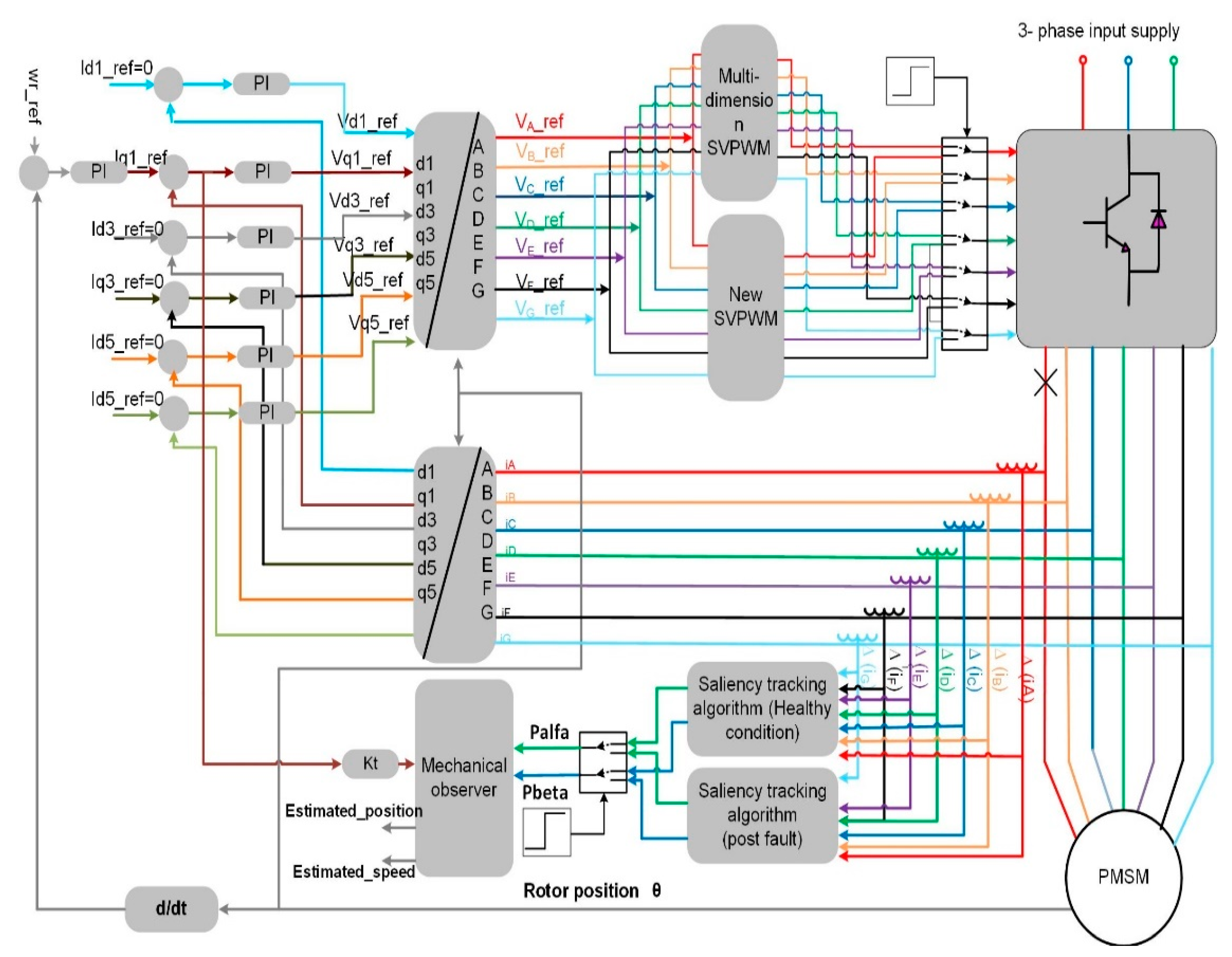
3.3. Simulation Results of the Speed Control of the Seven-Phase Drive after Losing Phase ‘A’

The new SVPWM algorithm that is proposed in the above section has been implemented using SABER simulator as shown in Figure 12. When the motor is running under healthy operating conditions, the multi-dimension space vector modulation will be used. If phase ‘A’ is disconnected due to the open-circuit fault, then the new space vector modulation is implemented as a part of the fault-tolerant technique. It should be mentioned here that the switching frequency for both the multi-dimension space vector modulation and the new space vector modulation was 5 kHz. The result of implementing the control structure depicted in Figure 12 is shown in Figure 13. The speed of the seven-phase motor was controlled to 120 rpm while the load was half without faults. And the NSV-SVPWM was used to generate the gate signals to the seven-phase inverter switches. Then at t = 1.5 s, an open-circuit fault was introduced to phase ‘A’ without changing the SVPWM technique. Although the motor continued operation, the stator currents in this period were unbalanced and some of them increased by 50% compared to the currents under healthy operating condition. Moreover, the ripples in speed and torque were increased too. At t = 2.5 s, the new SVPWM technique proposed in this paper was used. It can be seen that the remaining currents became equal in magnitudes and the new amplitude of the remaining currents has increased by 23% compared to the currents under healthy operating conditions. Also, the phase shifts between the currents were changed too and became similar to those obtained in Figure 7 (i.e., under minimum inverter current limitation optimization technique). Finally, the ripple in speed and torque was improved using the new SVPWM technique.

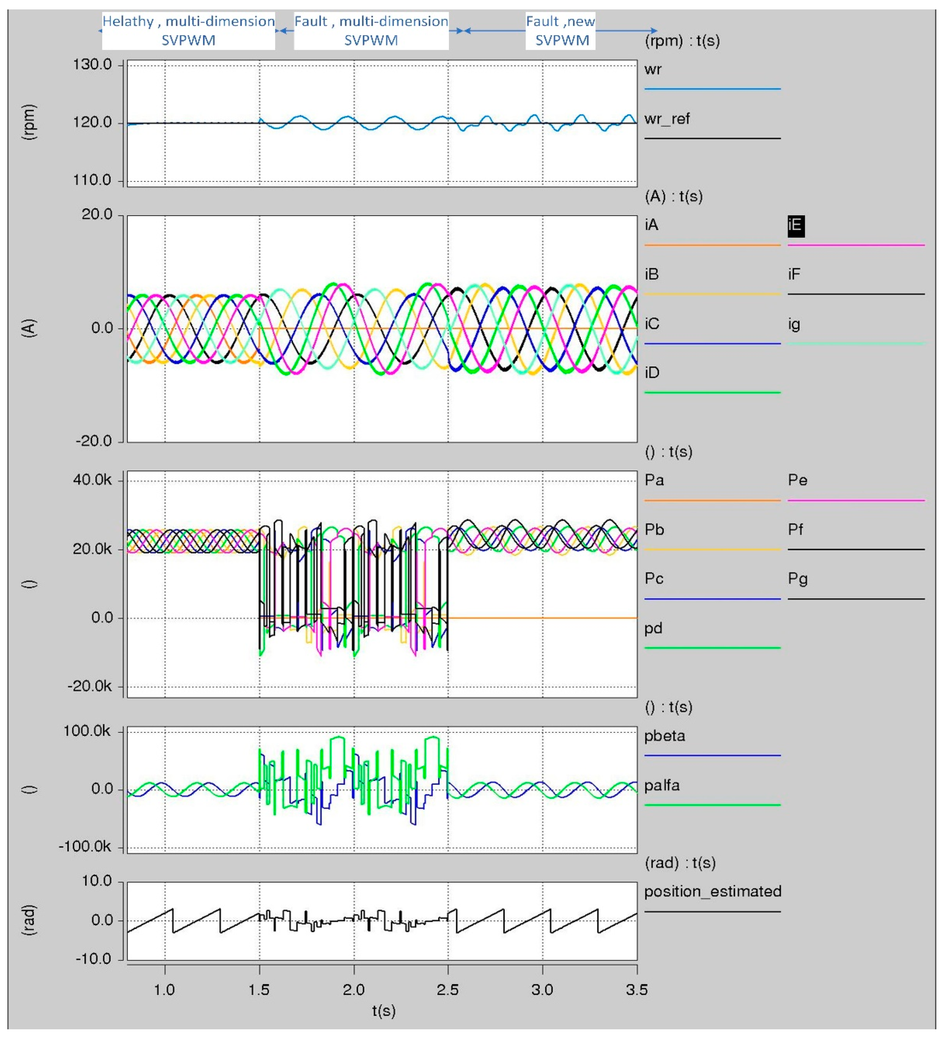
4. Saliency Position Tracking in the Seven-Phase Motor Post the Fault

4.1. Saliecy-Tracking Algorithm Post the Failure

The algorithm that has been developed in [38] to obtain the rotor speed and position in the seven-phase motor running without faults will not be applicable after losing phase ‘A’. This is related to the fact that it depends on measuring the derivative of the stator currents due to the inverter switching actions to track the saliency position. While the derivative of the current in phase ‘A’ will be zero due to the open circuit. Moreover, the use of the new SVPWM post the fault as a part of the FTC technique will change the inverter switching actions, so it affects the algorithm to track the saliency. To solve these problems, a new algorithm to track the saliency in the seven-phase motor after losing phase ’A’ is presented. The new algorithm is based on the new SVPWM technique introduced in this paper.

Figure 14a shows how the adjacent active vectors in addition to the null vectors are used to synthesize V_ref in the first sector. While Figure 10b shows the PWM waveform associated with applying these vectors and it shows the sampling instant of the derivative of the stator currents.

The dynamic circuits of the stator windings of the seven-phase motor after losing phase ‘A’ during the application of the vector V0, V3, V1, V5, V2, and V4 are shown in the Figure 15a, Figure 15b, Figure 15c, Figure 15d, Figure 15e, and Figure 15f respectively. Using the circuits in these figures, the equations below hold true:

$$\left[0\right]=r_s\ast \left[\begin{array}{c}{i}_B{}^{\left(V0\right)}\end{array}\right]+\left[\begin{array}{c}{l}_{\sigma B}\ast \Delta \left(i_B{}^{\left(V0\right)}\right)\end{array}\right]+\left[\begin{array}{c}{e}_B{}^{\left(V0\right)}\end{array}\right]$$

(13)

$$\left[\begin{array}{c}VDC\\ 0\end{array}\right]=r_s\ast \left[\begin{array}{c}{i}_B{}^{\left(V3\right)}\\ i_G{}^{\left(V3\right)}\end{array}\right]+\left[\begin{array}{c}{l}_{\sigma B}\ast \Delta \left(i_B{}^{\left(V3\right)}\right)\\ l_{\sigma G}\ast \Delta \left(i_G{}^{\left(V3\right)}\right)\end{array}\right]+\left[\begin{array}{c}{e}_B{}^{\left(V3\right)}\\ e_G{}^{\left(V3\right)}\end{array}\right]$$

(14)

$$\left[\begin{array}{c}VDC\\ 0\end{array}\right]=r_s\ast \left[\begin{array}{c}{i}_G{}^{\left(V1\right)}\\ i_C{}^{\left(V1\right)}\end{array}\right]+\left[\begin{array}{c}{l}_{\sigma G}\ast \Delta \left(i_G{}^{\left(V1\right)}\right)\\ l_{\sigma C}\ast \Delta \left(i_C{}^{\left(V1\right)}\right)\end{array}\right]+\left[\begin{array}{c}{e}_G{}^{\left(V1\right)}\\ e_C{}^{\left(V1\right)}\end{array}\right]$$

(15)

$$\left[\begin{array}{c}VDC\\ 0\end{array}\right]=r_s\ast \left[\begin{array}{c}{i}_C{}^{\left(V5\right)}\\ i_F{}^{\left(V5\right)}\end{array}\right]+\left[\begin{array}{c}{l}_{\sigma C}\ast \Delta \left(i_C{}^{\left(V5\right)}\right)\\ l_{\sigma F}\ast \Delta \left(i_F{}^{\left(V5\right)}\right)\end{array}\right]+\left[\begin{array}{c}{e}_C{}^{\left(V5\right)}\\ e_F{}^{\left(V5\right)}\end{array}\right]$$

(16)

$$\left[\begin{array}{c}VDC\\ 0\end{array}\right]=r_s\ast \left[\begin{array}{c}{i}_F{}^{\left(V2\right)}\\ i_D{}^{\left(V2\right)}\end{array}\right]+\left[\begin{array}{c}{l}_{\sigma F}\ast \Delta \left(i_F{}^{\left(V2\right)}\right)\\ l_{\sigma D}\ast \Delta \left(i_D{}^{\left(V2\right)}\right)\end{array}\right]+\left[\begin{array}{c}{e}_F{}^{\left(V2\right)}\\ e_D{}^{\left(V2\right)}\end{array}\right]$$

(17)

$$\left[\begin{array}{c}VDC\\ 0\end{array}\right]=r_s\ast \left[\begin{array}{c}{i}_D{}^{\left(V4\right)}\\ i_E{}^{\left(V4\right)}\end{array}\right]+\left[\begin{array}{c}{l}_{\sigma D}\ast \Delta \left(i_D{}^{\left(V4\right)}\right)\\ l_{\sigma E}\ast \Delta \left(i_E{}^{\left(V4\right)}\right)\end{array}\right]+\left[\begin{array}{c}{e}_D{}^{\left(V4\right)}\\ e_E{}^{\left(V4\right)}\end{array}\right]$$

(18)

$$\left[VDC\right]=r_s\ast \left[\begin{array}{c}{i}_E{}^{\left(V0\right)}\end{array}\right]+\left[\begin{array}{c}{l}_{\sigma E}\ast \Delta \left(i_E{}^{\left(V0\right)}\right)\end{array}\right]+\left[\begin{array}{c}{e}_E{}^{\left(V0\right)}\end{array}\right]$$

(19)

where $l_{\sigma }$ and e is the stator leakage inductance and the back emf per phase.

By subtracting each two adjacent equations from each other, the following equations can be derived.

$$\left[\begin{array}{c}VDC\\ VDC\\ VDC\\ VDC\\ VDC\\ VDC\end{array}\right]=r_s\ast \left[\begin{array}{c}{i}_B{}^{\left(V3\right)}-i_B{}^{\left(V0\right)}\\ \begin{array}{c}{i}_C{}^{\left(V5\right)}-i_C{}^{\left(V1\right)}\end{array}\\ \begin{array}{c}{i}_D{}^{\left(V4\right)}-i_D{}^{\left(V2\right)}\end{array}\\ \begin{array}{c}{i}_E{}^{\left(V0\right)}-i_E{}^{\left(V4\right)}\\ i_F{}^{\left(V2\right)}-i_F{}^{\left(V5\right)}\\ i_G{}^{\left(V1\right)}-i_G{}^{\left(V3\right)}\end{array}\end{array}\right]+\left[\begin{array}{c}{l}_{\sigma B}\ast \Delta \left(i_B{}^{\left(V3\right)}-i_B{}^{\left(V0\right)}\right)\\ l_{\sigma C}\ast \Delta \left(i_C{}^{\left(V5\right)}-i_C{}^{\left(V1\right)}\right)\\ l_{\sigma D}\ast \Delta \left(i_D{}^{\left(V4\right)}-i_D{}^{\left(V2\right)}\right)\\ l_{\sigma E}\ast \Delta \left(i_E{}^{\left(V0\right)}-i_E{}^{\left(V4\right)}\right)\\ l_{\sigma F}\ast \Delta \left(i_F{}^{\left(V2\right)}-i_F{}^{\left(V5\right)}\right)\\ l_{\sigma G}\ast \Delta \left(i_G{}^{\left(V1\right)}-i_G{}^{\left(V3\right)}\right)\end{array}\right]+\left[\begin{array}{c}\begin{array}{c}{e}_B{}^{\left(V3\right)}-e_B{}^{\left(V0\right)}\end{array}\\ \begin{array}{c}{e}_C{}^{\left(V5\right)}-e_C{}^{\left(V1\right)}\end{array}\\ e_D{}^{\left(V4\right)}-e_D{}^{\left(V2\right)}\\ e_E{}^{\left(V0\right)}-e_E{}^{\left(V4\right)}\\ e_F{}^{\left(V2\right)}-e_F{}^{\left(V5\right)}\\ e_G{}^{\left(V1\right)}-e_G{}^{\left(V3\right)}\end{array}\right]$$

(20)

If the drop voltage across the $r_s$ is neglected as it will be very small in addition to neglecting the terms related to the back emf as there will be little change in the back emf between the vectors, Equation (20) can be written as:

$$\left[\begin{array}{c}VDC\\ VDC\\ VDC\\ VDC\\ VDC\\ VDC\\ VDC\end{array}\right]=\left[\begin{array}{c}{l}_{\sigma B}\ast \Delta \left(i_B{}^{\left(V3\right)}-i_B{}^{\left(V0\right)}\right)\\ l_{\sigma C}\ast \Delta \left(i_C{}^{\left(V5\right)}-i_C{}^{\left(V1\right)}\right)\\ l_{\sigma D}\ast \Delta \left(i_D{}^{\left(V4\right)}-i_D{}^{\left(V2\right)}\right)\\ l_{\sigma E}\ast \Delta \left(i_E{}^{\left(V0\right)}-i_E{}^{\left(V4\right)}\right)\\ l_{\sigma F}\ast \Delta \left(i_F{}^{\left(V2\right)}-i_F{}^{\left(V5\right)}\right)\\ l_{\sigma G}\ast \Delta \left(i_G{}^{\left(V1\right)}-i_G{}^{\left(V3\right)}\right)\end{array}\right]$$

(21)

The position scalars $P_B$, $P_C$, $P_D$, $P_E$, $P_F$, and $P_G$ can be constructed as follows:

$$\left[\begin{array}{c}{P}_B\\ P_C\\ P_D\\ P_E\\ P_F\\ P_G\end{array}\right]=C\ast \left[\begin{array}{c}\Delta \left(i_B{}^{\left(V3\right)}-i_B{}^{\left(V0\right)}\right)\\ \Delta \left(i_C{}^{\left(V5\right)}-i_C{}^{\left(V1\right)}\right)\\ \Delta \left(i_D{}^{\left(V4\right)}-i_D{}^{\left(V2\right)}\right)\\ \Delta \left(i_E{}^{\left(V0\right)}-i_E{}^{\left(V4\right)}\right)\\ \Delta \left(i_F{}^{\left(V2\right)}-i_F{}^{\left(V5\right)}\right)\\ \Delta \left(i_G{}^{\left(V1\right)}-i_G{}^{\left(V3\right)}\right)\end{array}\right]$$

(22)

where

$$C=\frac{VDC-L_{so}+L_{sl}}{L_x}$$

(23)

These position scalars can be used to obtain $\alpha ,$ $\beta$ components of the saliency position as follows:

$$\left[\begin{array}{c}{P}_{\alpha }\\ P_{\beta }\end{array}\right]=\left[V\right]\left[\begin{array}{c}{P}_B\\ P_C\\ P_D\\ P_E\\ P_F\\ P_G\end{array}\right]$$

(24)

where

$$V=\left[\begin{array}{c}\begin{array}{cc}\cos \left(4\pi /7\right)& \cos \left(8\pi /7\right)\end{array}\begin{array}{cc}\cos \left(12\pi /7\right)& \cos \left(2\pi /7\right)\end{array}\cos \left(6\pi /7\right)\cos \left(10/7\right)\\ \begin{array}{cc}\sin \left(4\pi /7\right)& \sin \left(8\pi /7\right)\end{array}\begin{array}{cc}\sin \left(12\pi /7\right)& \sin \left(2\pi /7\right)\end{array}\sin \left(6\pi /7\right)\sin \left(10\pi /7\right)\end{array}\right]$$

(25)

The algorithm to obtain the position signals in all sectors are given in

Table 3. Selection of the saliency position scalars after losing phase ‘A’ at different sectors.

Sector	${\mathit{P}}_{\mathit{B}}$	${\mathit{P}}_{\mathit{C}}$	${\mathit{P}}_{\mathit{D}}$	${\mathit{P}}_{\mathit{E}}$	${\mathit{P}}_{\mathit{F}}$	${\mathit{P}}_{\mathit{G}}$
1	$\Delta \left(i_B{}^{\left(V3\right)}-i_B{}^{\left(V0\right)}\right)$	$\Delta \left(i_C{}^{\left(V5\right)}-i_C{}^{\left(V1\right)}\right)$	$\Delta \left(i_D{}^{\left(V4\right)}-i_D{}^{\left(V2\right)}\right)$	$\Delta \left(i_E{}^{\left(V0\right)}-i_E{}^{\left(V4\right)}\right)$	$\Delta \left(i_F{}^{\left(V2\right)}-i_F{}^{\left(V5\right)}\right)$	$\Delta \left(i_G{}^{\left(V1\right)}-i_G{}^{\left(V3\right)}\right)$
2	$\Delta \left(i_B{}^{\left(V3\right)}-i_B{}^{\left(V0\right)}\right)$	$\Delta \left(i_C{}^{\left(V6\right)}-i_C{}^{\left(V3\right)}\right)$	$\Delta \left(i_D{}^{\left(V7\right)}-i_D{}^{\left(V5\right)}\right)$	$\Delta \left(i_E{}^{\left(V0\right)}-i_E{}^{\left(V4\right)}\right)$	$\Delta \left(i_F{}^{\left(V4\right)}-i_F{}^{\left(V7\right)}\right)$	$\Delta \left(i_G{}^{\left(V5\right)}-i_G{}^{\left(V6\right)}\right)$
3	$\Delta \left(i_B{}^{\left(V6\right)}-i_B{}^{\left(V8\right)}\right)$	$\Delta \left(i_C{}^{\left(V8\right)}-i_C{}^{\left(V0\right)}\right)$	$\Delta \left(i_D{}^{\left(V10\right)}-i_D{}^{\left(V6\right)}\right)$	$\Delta \left(i_E{}^{\left(V9\right)}-i_E{}^{\left(V7\right)}\right)$	$\Delta \left(i_F{}^{\left(V0\right)}-i_F{}^{\left(V9\right)}\right)$	$\Delta \left(i_G{}^{\left(V7\right)}-i_G{}^{\left(V10\right)}\right)$
4	$\Delta \left(i_B{}^{\left(V10\right)}-i_B{}^{\left(V11\right)}\right)$	$\Delta \left(i_C{}^{\left(V8\right)}-i_C{}^{\left(V0\right)}\right)$	$\Delta \left(i_D{}^{\left(V11\right)}-i_D{}^{\left(V8\right)}\right)$	$\Delta \left(i_E{}^{\left(V12\right)}-i_E{}^{\left(V10\right)}\right)$	$\Delta \left(i_F{}^{\left(V0\right)}-i_F{}^{\left(V9\right)}\right)$	$\Delta \left(i_G{}^{\left(V9\right)}-i_G{}^{\left(V12\right)}\right)$
5	$\Delta \left(i_B{}^{\left(V12\right)}-i_B{}^{\left(V13\right)}\right)$	$\Delta \left(i_C{}^{\left(V11\right)}-i_C{}^{\left(V14\right)}\right)$	$\Delta \left(i_D{}^{\left(V14\right)}-i_D{}^{\left(V0\right)}\right)$	$\Delta \left(i_E{}^{\left(V13\right)}-i_E{}^{\left(V11\right)}\right)$	$\Delta \left(i_F{}^{\left(V15\right)}-i_F{}^{\left(V12\right)}\right)$	$\Delta \left(i_G{}^{\left(V0\right)}-i_G{}^{\left(V15\right)}\right)$
6	$\Delta \left(i_B{}^{\left(V15\right)}-i_B{}^{\left(V17\right)}\right)$	$\Delta \left(i_C{}^{\left(V13\right)}-i_C{}^{\left(V16\right)}\right)$	$\Delta \left(i_D{}^{\left(V14\right)}-i_D{}^{\left(V0\right)}\right)$	$\Delta \left(i_E{}^{\left(V16\right)}-i_E{}^{\left(V14\right)}\right)$	$\Delta \left(i_F{}^{\left(V17\right)}-i_F{}^{\left(V13\right)}\right)$	$\Delta \left(i_G{}^{\left(V0\right)}-i_G{}^{\left(V15\right)}\right)$
7	$\Delta \left(i_B{}^{\left(V0\right)}-i_B{}^{\left(V19\right)}\right)$	$\Delta \left(i_C{}^{\left(V17\right)}-i_C{}^{\left(V20\right)}\right)$	$\Delta \left(i_D{}^{\left(V16\right)}-i_D{}^{\left(V18\right)}\right)$	$\Delta \left(i_E{}^{\left(V18\right)}-i_E{}^{\left(V0\right)}\right)$	$\Delta \left(i_F{}^{\left(V20\right)}-i_F{}^{\left(V16\right)}\right)$	$\Delta \left(i_G{}^{\left(V19\right)}-i_G{}^{\left(V17\right)}\right)$
8	$\Delta \left(\left(i_B{}^{\left(V0\right)}-i_B{}^{\left(V19\right)}\right)\right)$	$\Delta \left(i_C{}^{\left(V19\right)}-i_C{}^{\left(V22\right)}\right)$	$\Delta \left(i_D{}^{\left(V20\right)}-i_D{}^{\left(V21\right)}\right)$	$\Delta \left(i_E{}^{\left(V18\right)}-i_E{}^{\left(V0\right)}\right)$	$\Delta \left(i_F{}^{\left(V21\right)}-i_F{}^{\left(V18\right)}\right)$	$\Delta \left(i_G{}^{\left(V22\right)}-i_G{}^{\left(V20\right)}\right)$
9	$\left(i_B{}^{\left(V24\right)}-i_B{}^{\left(V22\right)}\right)$	$\Delta \left(i_C{}^{\left(V0\right)}-i_C{}^{\left(V24\right)}\right)$	$\Delta \left(i_D{}^{\left(V22\right)}-i_D{}^{\left(V25\right)}\right)$	$\Delta \left(i_E{}^{\left(V21\right)}-i_E{}^{\left(V23\right)}\right)$	$\Delta \left(i_F{}^{\left(V23\right)}-i_F{}^{\left(V0\right)}\right)$	$\Delta \left(i_G{}^{\left(V25\right)}-i_G{}^{\left(V21\right)}\right)$
10	$\Delta \left(i_B{}^{\left(V27\right)}-i_B{}^{\left(V25\right)}\right)$	$\Delta \left(i_C{}^{\left(V0\right)}-i_C{}^{\left(V27\right)}\right)$	$\Delta \left(i_D{}^{\left(V24\right)}-i_D{}^{\left(V27\right)}\right)$	$\Delta \left(i_E{}^{\left(V25\right)}-i_E{}^{\left(V23\right)}\right)$	$\Delta \left(i_F{}^{\left(V23\right)}-i_F{}^{\left(V0\right)}\right)$	$\Delta \left(i_G{}^{\left(V26\right)}-i_G{}^{\left(V23\right)}\right)$
11	$\Delta \left(i_B{}^{\left(V28\right)}-i_B{}^{\left(V26\right)}\right)$	$\Delta \left(i_C{}^{\left(V30\right)}-i_C{}^{\left(V27\right)}\right)$	$\Delta \left(i_D{}^{\left(V0\right)}-i_D{}^{\left(V30\right)}\right)$	$\Delta \left(i_E{}^{\left(V27\right)}-i_E{}^{\left(V28\right)}\right)$	$\Delta \left(i_F{}^{\left(V26\right)}-i_F{}^{\left(V29\right)}\right)$	$\Delta \left(i_G{}^{\left(V29\right)}-i_G{}^{\left(V0\right)}\right)$
12	$\Delta \left(i_B{}^{\left(V1\right)}-i_B{}^{\left(V29\right)}\right)$	$\Delta \left(i_C{}^{\left(V2\right)}-i_C{}^{\left(V28\right)}\right)$	$\Delta \left(i_D{}^{\left(V0\right)}-i_D{}^{\left(V30\right)}\right)$	$\Delta \left(i_E{}^{\left(V30\right)}-i_E{}^{\left(V2\right)}\right)$	$\Delta \left(i_F{}^{\left(V28\right)}-i_F{}^{\left(V1\right)}\right)$	$\Delta \left(i_G{}^{\left(V29\right)}-i_G{}^{\left(V0\right)}\right)$

.

4.2. Simulation Results of the Saliecy-Tracking Algorithm after Losing Phase ‘A’

The proposed algorithm given in Table 3 to track the saliency in the seven-phase motor drive after losing phase ‘A’ and using the new SVPWM technique has been simulated in Saber according to the control structure shown in Figure 16. The transient current responses (∆($i_A$, $i_B$, $i_C$, $i_D$, $i_E$, $i_F$, and $i_G$) of the PMSM were measured. Then according to the operating condition of the seven-phase motor drive (i.e., healthy or after losing phase ‘A’) the algorithm to track the saliency is chosen. Moreover, a mechanical observer [45] was used to suppress any noise encountered in the estimated position signals. Note the simulation includes a minimum pulse width of 10 us when the derivative of the motors currents were sampled.

The simulation results obtained from this control structure are depicted in Figure 17. Firstly, the motor was running without faults (i.e., the NSV-SVPWM and the algorithm presented in [36] were used to track the saliency). At t = 1.5 s, phase ‘A’ of the seven-phase motor drive was lost without using new SVPWM and the new algorithm to track the saliency. Finally, at t = 2.5 s, both the new SVPWM technique and the new algorithm to track the saliency were implemented. It is obvious from the results that the saliency was not be able to track after losing phase ‘A’ without using the new algorithm presented in this paper. Moreover, the quality of the position signals after losing phase ‘A’ obtained by the new algorithm was as good as those obtained when the motor was running without faults.

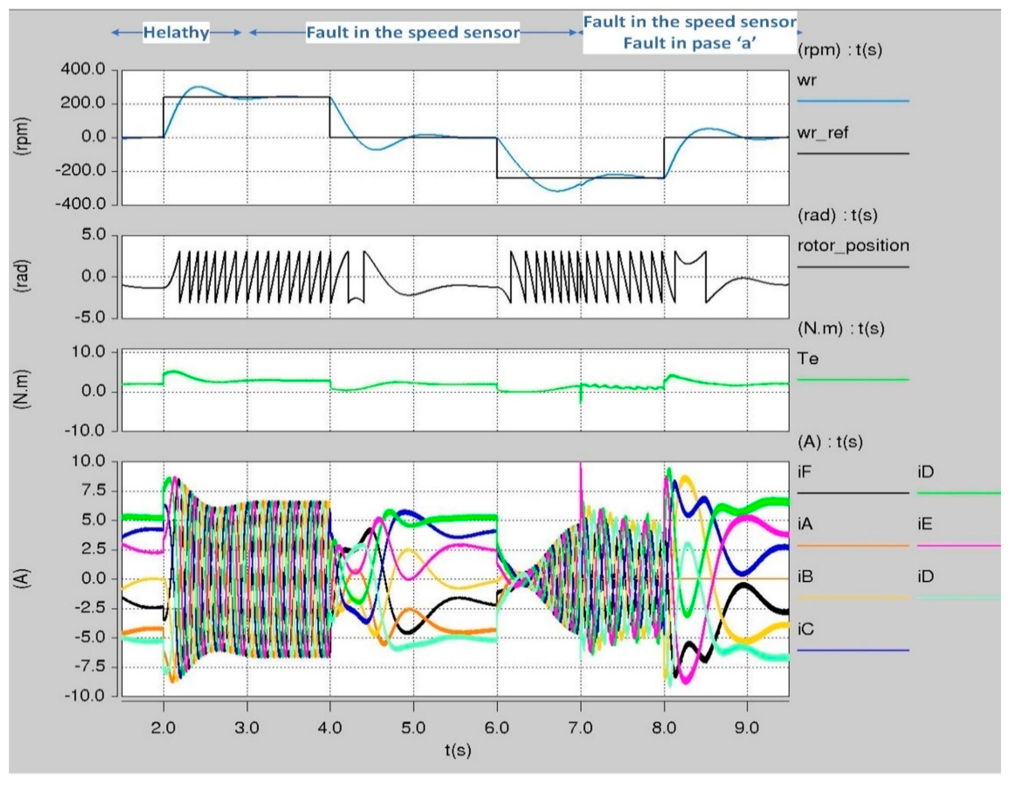
5. Simulation Results of the Seven-Phase Drive after Losing Phase ‘A’ and the Speed Sensor

The closed-loop speed control of the seven-phase drive post the failures in phase ‘A’ and the speed sensor has been simulated using SABER simulator based on the control structure shown in Figure 18. The NSV-SVPWM in addition to the saliency tracking algorithm proposed in [38] will be used if the motor is operated without faults. When the failure in phase ‘A’ is introduced, then the new SVPWM technique proposed in Section 3 and the new algorithm to track the saliency proposed in Section 4 will be used.

The figures below demonstrate the performance of the seven-phase drive after losing phase ‘A’ and losing the speed sensor due to the faults at different load and speed conditions. Figure 19 shows the response of the seven-phase drive post the faults at low speeds. From the beginning until t = 3 s, the motor was operating at speed = −30 rpm without faults. At t = 3 s, the speed of the drive was reversed while the motor still running without faults. Then at t = 4.5 s, phase ‘A’ was lost due to the fault while the new SVPWM was used to assure the minimum inverter current optimization. After that, at t = 6 s and while phase ‘A’ was still lost, the speed of the drive was reversed again. At t = 7 s, an additional fault was introduced to the operation of the motor drive which is the failure in the speed sensor (i.e., the motor became running under the failures in phase ‘A’ and the speed sensor). Finally, at t = 9 s, and while the motor was running post the two failures, the speed of the motor drive was reversed for the third time. The results show the dynamic response in addition to the steady-state response of the whole drive post the two failures were as good as that obtained without failures. Moreover, the result proves the significant increase in the robustness of the drive by using the new SVPWM and the new technique to track the saliency.

Figure 20 shows a similar result to those obtained in Figure 19 but at higher speed steps. The drive was operating without faults at zero speed. At t = 2 s, the speed of the motor drive was changed to 240 rpm. Then, at t = 3 s, a fault in the speed sensor was introduced to the drive. Hence, the motor speed and position were obtained using the algorithm proposed in [36]. After that, two-speed steps from 240 rpm to 0 and from 0 to −240 rpm were applied to the motor drive while the speed sensor is still a failure. At t = 7 s, an additional failure in phase ‘A’ was introduced to the motor and the motor became running under the failures in the speed sensor in phase ‘A’. It should be mentioned here that after phase ‘A’ was disconnected, the new SVPWM proposed in this paper was used to assure the minimum inverter current optimization and at the same time, the algorithm proposed in this paper was used to obtain the rotor position and rotor speed. Finally, at t = 8 s, the reference speed of the motor drive was changed to 0. The dynamic and the steady-state responses of the whole drive system illustrated in Figure 20 post the failures were at the same quality of the response of the drive system when running without faults.

Figure 21 illustrates the robustness of the seven-phase drive when a load disturbance is applied post the failures. The motor was running at −90 rpm without faults. At t = 2 s, phase ‘A’ was disconnected due to an open-circuit fault. After that and while the phase ‘a’ was disconnected, a load disturbance was applied to the seven-phase drive and then removed between t = 3 s and t = 4.5 s. Then the motor speed was controlled to 0 rpm at t = 6.5 s. While the motor was running at zero speed and phase ‘A’ was disconnected, an additional fault was introduced to the seven-phase drive at t = 7 s which was the fault in the speed sensor. At t = 7.5 s the speed of the motor was controlled to 90 rpm. Finally, while the motor was running post the failures in the speed sensor in phase ‘A’, a load disturbance was applied to the seven-phase drive and then removed between t = 8 s and t = 9.5 s. the results in Figure 21 show that during the whole test the motor drive speed was maintained during the application of the load disturbance even though the motor drive was running post the failure in the speed sensor and post the failure in phase ‘A’.

6. Conclusions

This paper has proposed a new FTC strategy for the seven-phase PMSM motor drive to keep it operational in the event of two types of faults happening at the same time. This FTC strategy is divided into two parts. The first part is to maintain the operation of the seven-phase motor drive after losing phase ‘A’ based on minimum inverter current optimization technique. This part has been achieved through the new SVPMW technique that has been proposed in this paper. The second part of the FTC strategy was to maintain the operation of the whole drive after the failure in the speed sensor. This has been achieved by developing an algorithm to track the saliency after losing phase ’A’. The results have shown that the ripple in speed after the fault was reduced from ±4 rpm to ±2 rpm when the new FTC was used. Additionally, the frequency of the torque ripple has been increased and the magnitude is decreased from ±0.2 N.m to ±0.1 N.m. In addition, the amplitude of the currents has been limited to 1.23 times the amplitude of the current before the fault. Finally, it worth mentioning that the implementation of this technique is quite easy and can be implemented to the induction motor too.

References

1. Villani, M.; Tursini, M.; Fabri, G.; Castellini, L. Multi-phase fault tolerant drives for aircraft applications. In Proceedings of the Electrical Systems for Aircraft, Railway and Ship Propulsion conference, Bologna, Italy, 19–21 October 2010; pp. 1–6. [Google Scholar]
2. Levi, E.; Bojoi, R.; Profumo, F.; Toliyat, H.A.; Williamson, S. Multiphase induction motor drives—A technology status review. IET Electr. Power Appl. 2007, 1, 489–516. [Google Scholar] [CrossRef] [Green Version]
3. Subotic, I.; Bodo, N.; Levi, E.; Jones, M. Onboard Integrated Battery Charger for EVs Using an Asymmetrical Nine-Phase Machine. IEEE Trans. Ind. Electron. 2015, 62, 3285–3295. [Google Scholar] [CrossRef]
4. Yepes, A.G.; Lopez, O.; Gonzalez-Prieto, I.; Duran, M.J.; Doval-Gandoy, J. A Comprehensive Survey on Fault Tolerance in Multiphase AC Drives, Part 1: General Overview Considering Multiple Fault Types. Machines 2022, 10, 208. [Google Scholar] [CrossRef]
5. Abdel-Khalik, A.S.; Elgenedy, M.A.; Ahmed, S.; Massoud, A.M. An Improved Fault Tolerant Five-Phase Induction Machine Using A Combined Star/Pentagon Single Layer Stator Winding Connection. IEEE Trans. Ind. Electron. 2015, 63, 618–628. [Google Scholar] [CrossRef]
6. Yepes, A.G.; Gonzalez-Prieto, I.; Lopez, O.; Duran, M.J.; Doval-Gandoy, J. A Comprehensive Survey on Fault Tolerance in Multiphase AC Drives, Part 2: Phase and Switch Open-Circuit Faults. Machines 2022, 10, 221. [Google Scholar] [CrossRef]
7. Iftikhar, M.H.; Park, B.-G.; Kim, J.-W. Design and Analysis of a Five-Phase Permanent-Magnet Synchronous Motor for Fault-Tolerant Drive. Energies 2021, 14, 514. [Google Scholar] [CrossRef]
8. Huang, X.; Goodman, A.; Gerada, C.; Fang, Y.; Lu, Q. Design of a Five-Phase Brushless DC Motor for a Safety Critical Aerospace Application. IEEE Trans. Ind. Electron. 2012, 59, 3532–3541. [Google Scholar] [CrossRef]
9. Shao, L.; Hua, W.; Dai, N.; Shao, L. Mathematical Modeling of a 12-Phase Machine for Wind Power Generation. IEEE Trans. Ind. Electron. 2016, 63, 504–516. [Google Scholar] [CrossRef]
10. Pantea, A.; Yazidi, A.; Betin, F.; Taherzadeh, M.; Carrière, S.; Henao, H.; Capolino, G.A. Six-Phase Induction Machine Model for Electrical Fault Simulation Using the Circuit-Oriented Method. IEEE Trans. Ind. Electron. 2016, 63, 494–503. [Google Scholar] [CrossRef]
11. Che, H.S.; Duran, M.J.; Levi, E.; Jones, M.; Hew, W.; Rahim, N.A. Postfault Operation of an Asymmetrical Six-Phase Induction Machine With Single and Two Isolated Neutral Points. IEEE Trans. Power Electron. 2014, 29, 5406–5416. [Google Scholar] [CrossRef] [Green Version]
12. Che, H.S.; Levi, E.; Jones, M.; Hew, W.; Rahim, N.A. Current Control Methods for an Asymmetrical Six-Phase Induction Motor Drive. IEEE Trans. Power Electron. Trans. Power Electron. 2014, 29, 407–417. [Google Scholar] [CrossRef] [Green Version]
13. Gonzalez-Prieto, I.; Duran, M.J.; Che, H.S.; Levi, E.; Bermúdez, M.; Barrero, F. Fault-Tolerant Operation of Six-Phase Energy Conversion Systems With Parallel Machine-Side Converters. IEEE Trans. Power Electron. 2016, 31, 3068–3079. [Google Scholar] [CrossRef] [Green Version]
14. Liu, Z.; Houari, A.; Machmoum, M.; Benkhoris, M.F.; Tang, T. An active FTC strategy using generalized proportional integral observers applied to five-phase PMSG based tidal current energy conversion systems. Energies 2020, 13, 6645. [Google Scholar] [CrossRef]
15. Jinquan, X.; Boyi, Z.; Hao, F.; Hong, G. Guaranteeing the fault transient performance of aerospace multiphase permanent magnet motor system: An adaptive robust speed control approach. CES Trans. Electr. Mach. Syst. 2020, 4, 114–122. [Google Scholar]
16. Mossa, M.A.; Echeikh, H.; Diab, A.A.Z.; Haes Alhelou, H.; Siano, P. Comparative Study of Hysteresis Controller, Resonant Controller and Direct Torque Control of Five-Phase IM under Open-Phase Fault Operation. Energies 2021, 14, 1317. [Google Scholar] [CrossRef]
17. Baudart, F.; Dehez, B.; Matagne, E.; Telteu-nedelcu, D.; Alexandre, P.; Labrique, F. Torque Control Strategy of Polyphase Permanent-Magnet Synchronous Machines With Minimal Controller Reconfiguration Under Open-Circuit Fault of One Phase. IEEE Trans. Ind. Electron. 2012, 59, 2632–2644. [Google Scholar] [CrossRef]
18. Jia, H.; Yang, J.; Deng, R.; Wang, Y. Loss Investigation for Multiphase Induction Machine under Open-Circuit Fault Using Field–Circuit Coupling Finite Element Method. Energies 2021, 14, 5686. [Google Scholar] [CrossRef]
19. Fu, J.R.; Lipo, T.A. Disturbance-Free Operation of a Multiphase Current-Regulated Motor Drive with an Opened Phase. IEEE Trans. Ind. Appl. 1994, 30, 1267–1274. [Google Scholar]
20. Zheng, L.; Fletcher, J.E.; Williams, B.W. Current Optimization for a Multi-Phase Machine under an Open Circuit Phase Fault Condition. In Proceedings of the 3rd IET International Conference on Power Electronics, Machines and Drives (PEMD 2006), Dublin, Ireland, 4–6 April 2006; pp. 414–419. [Google Scholar]
21. Mohammadpour, A.; Sadeghi, S.; Parsa, L. A Generalized Fault-Tolerant Control Strategy for Five-Phase PM Motor Drives Considering Star, Pentagon, and Pentacle Connections of Stator Windings. IEEE Trans. Ind. Electron. 2014, 61, 63–75. [Google Scholar] [CrossRef]
22. Abdel-Khalik, A.; Ahmed, S.; Elserougi, A.; Massoud, A. Effect of Stator Winding Connection of Five-Phase Induction Machines on Torque Ripples Under Open Line Condition. IEEE/ASME Trans. Mechatron. 2015, 20, 580–593. [Google Scholar] [CrossRef]
23. Sedrine, E.; Ojeda, J.; Gabsi, M.; Slama-Belkhodja, I. Fault-Tolerant Control Using the GA Optimization Considering the Reluctance Torque of a Five-Phase Flux Switching Machine. IEEE Trans. Energy Convers. 2015, 30, 927–938. [Google Scholar] [CrossRef]
24. Tian, B.; Hu, J.; Huang, X.; Zhou, B.; An, Q. Performance comparison of three types of PWM techniques for a Five-phase PMSM with a single-phase open circuited. In Proceedings of the 2021 13th International Symposium on Linear Drives for Industry Applications (LDIA), Wuhan, China, 1–3 July 2021; pp. 1–5. [Google Scholar] [CrossRef]
25. Chen, Q.; Liu, G.; Zhao, W.; Qu, L.; Xu, G. Asymmetrical SVPWM Fault-Tolerant Control of Five-Phase PM Brushless Motors. IEEE Trans. Energy Convers. 2017, 32, 12–22. [Google Scholar] [CrossRef]
26. Guzman, H.; Duran, M.; Barrero, F.; Zarri, L.; Bogado, B.; Prieto, I.; Arahal, M. Comparative study of predictive and resonant controllers in fault-tolerant five-phase induction motor drives. IEEE Trans. Ind. Electron. 2016, 63, 606–617. [Google Scholar] [CrossRef]
27. Cheng, L.; Sui, Y.; Zheng, P.; Wang, P.; Wu, F. Implementation of postfault decoupling vector control and mitigation of current ripple for five-phase fault-tolerant PM machine under single-phase open-circuit fault. IEEE Trans. Power Electron. 2018, 33, 8623–8636. [Google Scholar] [CrossRef]
28. Zhou, H.; Zhao, W.; Liu, G.; Cheng, R.; Xie, Y. Remedial field-oriented control of five-phase fault-tolerant permanent-magnet motor by using reduced-order transformation matrices. IEEE Trans. Ind. Electron. 2017, 64, 169–178. [Google Scholar] [CrossRef]
29. Chen, Q.; Zhao, W.; Liu, G.; Lin, Z. Extension of virtual-signal injection-based MTPA control for five-phase IPMSM into fault-tolerant operation. IEEE Trans. Ind. Electron. 2019, 66, 944–955. [Google Scholar] [CrossRef]
30. Chen, Q.; Gu, L.; Lin, Z.; Liu, G. Extension of space-vector signal-injection-based MTPA control into SVPWM fault-tolerant operation for five-phase IPMSM. IEEE Trans. Ind. Electron. 2020, 67, 7321–7333. [Google Scholar] [CrossRef]
31. Bermudez, M.; Gonzalez-Prieto, I.; Barrero, F.; Guzman, H.; Kestelyn, X.; Duran, M.J. An Experimental Assessment of Open-Phase Fault-Tolerant Virtual-Vector-Based Direct Torque Control in Five-Phase Induction Motor Drives. IEEE Trans. Power Electron. 2018, 33, 2774–2784. [Google Scholar] [CrossRef] [Green Version]
32. Tian, B.; Mirzaeva, G.; An, Q.; Sun, L.; Semenov, D. Fault-Tolerant Control of a Five-Phase Permanent Magnet Synchronous Motor for Industry Applications. IEEE Trans. Ind. Appl. 2018, 54, 3943–3952. [Google Scholar] [CrossRef]
33. Huang, W.; Hua, W.; Chen, F.; Yin, F.; Qi, J. Model Predictive Current Control of Open-Circuit Fault-Tolerant Five-Phase Flux- Switching Permanent Magnet Motor Drives. IEEE J. Emerg. Sel. Top. Power Electron. 2018, 6, 1840–1849. [Google Scholar] [CrossRef]
34. Zheng, L.; Fletcher, J.E.; Williams, B.W.; He, X. A novel direct torque control scheme for a sensorless five-phase induction motor drive. IEEE Trans. Ind. Electron. 2011, 58, 503–513. [Google Scholar] [CrossRef]
35. Mini, Y.; Nguyen, N.K.; Semail, E.; Vu, D.T. Enhancement of Sensorless Control for Non-Sinusoidal Multiphase Drives-Part I: Operation in Medium and High-Speed Range. Energies 2022, 15, 607. [Google Scholar] [CrossRef]
36. Almarhoon, A.H.; Zhu, Z.Q.; Xu, P. Improved rotor position estimation accuracy by rotating carrier signal injection utilizing zero-sequence carrier voltage for dual three-phase PMSM. IEEE Trans. Ind. Electron. 2017, 64, 4454–4462. [Google Scholar] [CrossRef]
37. Liu, G.; Geng, C.; Chen, Q. Sensorless Control for Five-Phase IPMSM Drives by Injecting HF Square-Wave Voltage Signal into Third Harmonic-Space. IEEE Access 2020, 8, 69712–69721. [Google Scholar] [CrossRef]
38. Saleh, K.; Sumner, M. Sensorless Control of Seven-Phase PMSM Drives Using NSV-SVPWM with Minimum Current Distortion. Electronics 2022, 11, 792. [Google Scholar] [CrossRef]
39. Saleh, K.; Sumner, M. Sensorless Speed Control of Five-Phase PMSM Drives in Case of a Single-Phase Open-Circuit Fault. Iran. J. Sci. Technol. Trans. Electr. Eng. 2019, 43, 501–517. [Google Scholar] [CrossRef]
40. Saleh, K.; Sumner, M. Sensorless Speed Control of a Fault-Tolerant Five-Phase PMSM Drives. Electr. Power Compon. Syst. 2020, 48, 919–932. [Google Scholar] [CrossRef]
41. Chen, K.Y. Multiphase pulse-width modulation considering reference order for sinusoidal wave production. In Proceedings of the 2015 IEEE 10th Conference on Industrial Electronics and Applications (ICIEA), Auckland, New Zealand, 15–17 June 2015; pp. 1155–1160. [Google Scholar]
42. Xue, S.; Wen, X.; Feng, Z. A Novel Multi-Dimensional SVPWM Strategy of Multiphase Motor Drives. In Proceedings of the 2006 12th International Power Electronics and Motion Control Conference, Portoroz, Slovenia, 30 August–1 September 2006; pp. 931–935. [Google Scholar]
43. Wang, P.; Zheng, P.; Wu, F.; Zhang, J.; Li, T. Research on dual-plane vector control of fivephase fault-tolerant permanent magnet machine. In Proceedings of the 2014 IEEE Conference and Expo Transportation Electrification Asia-Pacific (ITEC Asia-Pacific), Beijing, Chian, 31 August–3 September 2014; pp. 1–5. [Google Scholar]
44. Munim, W.N.W.A.; Che, H.S.; Hew, W.P. Fault tolerant capability of symmetrical multiphase machines under one open-circuit fault. In Proceedings of the 4th IET Clean Energy and Technology Conference (CEAT 2016), Kuala Lumpur, Malaysia, 14–15 November 2016; pp. 1–6. [Google Scholar] [CrossRef]
45. Lorenz, R.D.; Van Patten, K.W. High-resolution velocity estimation for all-digital, AC servo drives. IEEE Trans. Ind. Appl. 1991, 27, 701–705. [Google Scholar] [CrossRef]
Figure 1. Seven-phase drive topology.
Applsci 12 07979 g001
Figure 2. Voltage vector space distribution in the x1-y1 plane [38].
Applsci 12 07979 g002
Figure 3. (a) NSV-SVPWM vector synthesis in x1-y1, (b) PWM waveform [38].
Applsci 12 07979 g003
Figure 4. Current distribution of seven-phase motor under normal operating condition (a) Phasor; (b) sinusoidal.
Applsci 12 07979 g004
Figure 5. Current distribution of seven-phase motor under minimizing torque ripple optimization. (a) Phasor; (b) sinusoidal.
Applsci 12 07979 g005
Figure 6. Current distribution of seven-phase motor under minimizing copper losses optimization. (a) Phasor; (b) sinusoidal.
Applsci 12 07979 g006
Figure 7. Current distribution of seven-phase motor under minimizing inverter current optimization. (a) Phasor; (b) sinusoidal.
Applsci 12 07979 g007
Figure 8. Space vector diagram of the seven-phase PMSM after losing phase ‘A’.
Applsci 12 07979 g008
Figure 9. Flowchart illustrates the implementing the new SPVPWM after losing phase ‘A’.
Applsci 12 07979 g009
Figure 10. Illustration of how the adjacent active vectors are used to synthesis V_ref in the first sector using the new SVPWM after losing phase ‘A’. (a) active switching sequence. (b) PWM waveform.
Applsci 12 07979 g010
Figure 11. Synthesizing V_ref in the first sector using V3 and V1 only.
Applsci 12 07979 g011
Figure 12. Seven-phase drive control structure after losing phase ‘A’.
Applsci 12 07979 g012
Figure 13. Simulation results of using the new SVPWM technique for the seven-phase motor drive after losing phase ‘A’.
Applsci 12 07979 g013
Figure 14. Active switching sequence and the associated PWM waveform of the seven-phase drive after losing phase ‘A’ when V_ref exists in the first sector. (a) active switching sequence. (b) sampling instants.
Applsci 12 07979 g014
Figure 15. Dynamic equivalent of the seven-phase PMSM after losing phase ‘A’ when active vectors: (a) V0 is implemented; (b) V3 is implemented; (c) V1 is implemented; (d) V5 is implemented; (e) V2 is implemented; (f) V4 is implemented.
Applsci 12 07979 g015
Figure 16. Control structure to obtain the saliency position in seven-phase drive after losing phase ‘A’.
Applsci 12 07979 g016
Figure 17. Tracking the saliency of the seven-phase drive pre and post the losing of phase ‘A’.
Applsci 12 07979 g017
Figure 18. Speed control structure of the seven-phase drive after the faults.
Applsci 12 07979 g018
Figure 19. Low speed steps of the seven-phase drive post the failures in speed sensor and in phase ‘A’.
Applsci 12 07979 g019
Figure 20. High speed steps of the seven-phase motor drive post the failures in speed sensor and in phase ‘A’.
Applsci 12 07979 g020
Figure 21. Load steps post the failures in speed sensor and in phase ‘A’ of the seven-phase motor drive.
Applsci 12 07979 g021