1. Introduction
Modeling and simulation have become a key tool in many sciences and engineering disciplines [
1]. A simulation study is usually characterized by iterative model refinements, intertwined with problem analysis, conceptual modeling, and various experimentation activities, as illustrated in modeling and simulation life cycles [
2,
3,
4] (see
Figure 1). Due to their complexity, there is a high demand for approaches that allow simulation studies to be conducted in a more effective and systematic manner. Especially, support for conducting simulation experiments is of increasing interest, as they drive important activities, such as the calibration, validation, and analysis of models, and are essential for the reproducibility of simulation results.
With new computational power, the new availability of data, and the thereby strengthened role of simulation experiments in advancing science within the different application domains, the requirements referring to simulation studies and experiments are becoming more rigorous. In particular, there are increasing requirements regarding the correct usage of sensitivity and uncertainty analysis [
5], but also for calibration and validation to build realistic models [
6], as well as increasing demand for open, replicable, and transparent methodologies [
7]. In light of these new requirements, modelers that wish to create reproducible simulation experiments in an efficient and effective manner face new challenges. Especially, modelers working on interdisciplinary projects, where a variety of diverse simulation approaches and methods need to be brought together, would benefit from an easy-to-use tool that supports them in specifying, executing, and managing simulation experiments. However, also engineers working on modeling and simulation software have to account for these new challenges and would gain from a more structured and systematic approach for dealing with the increasing variety and complexity of the available specification languages (e.g., “Simulation Experiment Specification via a Scala Layer” [
8] and “Simulation Experiment Description Markup Language” [
9]), reporting guidelines (e.g., for finite element analysis studies in biomechanics [
10]), frameworks (e.g., the Simulation Automation Framework for Experiments [
11]), types of analyses and methods (e.g., experiment designs [
12]), and the myriad of applications, which require (partly) domain-specific solutions.
Model-driven-engineering (MDE)-based approaches can provide additional support in the specification, execution, and management of simulation experiments and resolve issues of interoperability, reproducibility, reusability, etc. In an MDE approach, meta models require certain experiment inputs, guide users through the experiment specification, and finally, generate executable code [
13]. Current MDE approaches for simulation experiments realize and demonstrate this for the generation of experiment designs for parameter scans [
13] and hypothesis testing [
14]. However, they concentrate on specific fields of simulation, support only a specific experiment type, or are tightly coupled with specific tools. As a consequence, their applicability and, thus, their impact on the way simulation experiments are conducted are limited. Furthermore, some typical benefits of MDE [
15], such as improved knowledge sharing and further automation, are not yet available or not fully exploited for simulation experiments. Thus, a more general approach is desirable that can support simulation experiments more broadly, and thus, assist in conducting entire simulation studies more effectively and systematically.
In this paper, we present a novel MDE framework that enhances the state-of-the-art of conducting simulation experiments in the following ways:
Improved knowledge sharing across domains: Experiment Meta models make knowledge about the structure and ingredients of simulation experiments explicit. By building various kinds of meta models and storing them in repositories, we allow modelers and developers to share knowledge about simulation experiments between the different communities, e.g., finite element analysis (FEA) or virtual prototyping. These usually develop their simulation methodology and tooling independently, although the way simulation experiments are specified and conducted rarely differ and, thus, could be supported by the same pipeline.
Increasing productivity and quality for complex experiments: For novice modelers, MDE clearly facilitates the specification of simulation experiments via targeted graphical user interfaces (GUIs) and code generation. We provide additional support via an experiment validator and allow for the support of complex simulation experiments via meta model composition. Due to the focus on complex experiments, also experienced modelers can benefit.
Reusability: The meta models give meaning to the ingredients of simulation experiments. Together with an easy-to-use, tool-independent format and a variety of backend bindings, we support the flexible and automatic reuse of simulation experiments. This is of interest when the performance of different simulation tools needs to be compared or model alternatives implemented using different modeling and simulation approaches shall be evaluated.
Automation: Further automation of simulation experiments can be achieved if the knowledge about the various simulation experiments (given by meta models) is put into relation with context knowledge about the simulation study (e.g., given by conceptual models [
16], provenance [
17], or documentation [
18]), as in these cases, simulation experiment specifications may be automatically generated and executed [
19]. As our approach provides a means for integration with various other frameworks, it presents a valuable basis for further automation of simulation experiments.
We demonstrate the above features and benefits of the approach using five experiments from three actual simulation studies. The studies are part of the Collaborative Research Centre (CRC) 1270 ELAINE (
https://www.elaine.uni-rostock.de/en/, accessed on 26 July 2022), which aims to develop novel electrically active implants for bone and cartilage regeneration, as well as for deep brain stimulation. As the research project is of an interdisciplinary nature, in each of the three studies, a different modeling and simulation approach and application domain are in focus (i.e., stochastic discrete-event simulation (DES) of a cell signaling pathway, virtual prototyping of a neurostimulator, and FEA of electric fields).
The paper is organized as follows. In
Section 2, we provide an overview of the related work. In
Section 3, we present the design of our novel model-driven approach for conducting simulation experiments. Details of the open-source implementation are given in
Section 4. In
Section 5, we demonstrate the benefits of our approach using three real simulation studies. Finally, we end the paper with conclusions and future work in
Section 6.
2. Related Work
Model-driven approaches for modeling and simulation so far have mostly focused on the generation of (executable) simulation models [
20,
21,
22,
23], simulation on distributed architectures [
24], or multi-formalism modeling [
25].
With regard to simulation experiments, MDE has been applied in the context of experiment design and hypothesis testing. Teran-Somohano et al. [
13] support the specification and execution of simple simulation experiments based on factorial designs, e.g., parameter sweeps. The approach by Dayıbaş et al. [
26] is based on one’s own domain-specific language for experiment design and semi-automatic transformations to multiple execution platforms. Yilmaz et al. [
14] propose the generation of experiment designs from hypotheses and outline an overarching goal–hypothesis–experiment framework.
Simulation experiments are also generated without explicit meta models or MDE frameworks. These usually target specific problems within the modeling and simulation life cycle. Lorig [
27], for instance, generates efficient experiment designs for hypothesis testing based on formally specified hypotheses. Peng et al. [
28] support the successive composition of models by generating simulation experiments for composed models. More specifically, statistical model checking experiments of individual models are reused and adapted for the composed model based on explicit experiment specifications and explicit behavioral properties. Similarly, properties of extended or refined models can be checked [
29]. Cooper et al. [
30] focus on supporting the comparison of electrophysiology models using typical experiment types of that domain, i.e., time course analyses and steady-state analysis. Concrete experiment specifications (protocols) conducted with previous models are stored in an online database and can be repeated with new models. Ruscheinski et al. [
18] present a pipeline for generating a number of different experiment types including local sensitivity analysis, optimization, and statistical model checking. This pipeline was expanded by experiment schemas in Wilsdorf et al. [
31] to support multiple simulation tools and approaches.
In this paper, we further generalize the latter experiment generation approach using the MDE paradigm. The main novelties are (a) the separation into two types of meta models (domain meta models and experiment type meta models) and a corresponding composition mechanism, (b) a meta model repository, (c) bi-directional transformations and execution bindings for a variety of tools, and (d) a command-line interface (CLI) for easy integration with other frameworks. As a result, our framework flexibly supports the conducting of diverse, complex experiment types, and it enables the sharing and reusing of knowledge even across different modeling domains and tools. Furthermore, our framework provides the foundation for automatically generating and reusing simulation experiments during the various phases of a simulation study, and thus for conducting entire simulation studies in a more systematic and effective manner.
The development of meta models, as part of an MDE framework, is closely related to the development of ontologies as both represent knowledge in a structured manner. Ontologies for modeling and simulation have been developed to facilitate the data exchange, interoperability, and annotation of simulation resources [
32]. Most ontologies define the components and concepts of simulation models instead of simulation experiments, e.g., the Discrete Event Simulation Component Ontology (DESC) [
33] or the Discrete-event Modeling Ontology (DeMO) [
34]. However, some ontologies overlap with meta models for simulation experiments, e.g., the ontology for capturing physics-based models by Cheong and Butscher [
35] and our meta model for FEA simulation studies (see
Section 5) both include the boundary condition and material properties.
3. Model-Driven Approach for Conducting Simulation Experiments
We developed a novel model-driven approach for conducting simulation experiments. Its central features are the separation into two types of meta models (domain meta models and experiment type meta models) and a corresponding composition mechanism, a meta model repository, bi-directional transformations and execution bindings for a variety of tools, and a CLI for easy integration with other frameworks. The approach as a whole can improve knowledge sharing across domains and approaches, increase productivity and quality for complex experiments, make simulation experiments reusable, and automatically generate and execute simulation experiments in various settings.
3.1. Framework Overview
Our approach for supporting the conducting of simulation experiments is based on the MDE principle. The central idea of MDE is combining meta models (i.e., a structured representation of concepts) with a means for code generation [
36]. Typically, MDE is realized in an architecture with four levels of abstraction and translations between them [
37].
Figure 2 illustrates our four-level MDE approach for simulation experiments. Experiment
meta models of the various domains and approaches of modeling and simulation are represented by the level
. In addition to the definition of these so-called
base experiments, meta models for a variety of
experiment types (e.g., sensitivity analysis (SA) or simulation-based optimization) exist. These two types of meta models can be composed flexibly to create meta models of complex simulation experiments. How meta models can be constructed is defined at the level of the
meta meta model (
), for example one could use formalisms such as UML class diagrams [
38] or schema languages [
39,
40] to express the meta models. However, experiment meta models are not only developed from scratch; therefore, we store them in a repository from which parts can be reused by related areas of simulation or by other experiment types. The newly developed meta models are again stored in the repository and thereby complement the knowledge collection about simulation experiments. A composed meta model (consisting of a base experiment and the experiment type) can be loaded via an interface (GUI or CLI). The loaded meta model dictates which inputs have to be provided to specify a valid simulation experiment. An experiment validator provides guidance for the modeler. If all inputs required by the meta model have been collected, a concrete tool-independent experiment specification (
model ) is generated. This general representation of the simulation experiment can now be easily reused, and some tools might also be able to import this specification directly. To receive an executable experiment
instance (
), the
-specification is automatically transformed to the code of a target backend and subsequently executed using the respective tool binding. In the following, we will describe the distinct features of our framework further.
3.2. Meta Modeling Language
At the highest level of abstraction in our framework, the meta meta model is situated. The meta meta model is essentially the language in which the meta models are specified. Meta meta models are usually self-referential (i.e., they define themselves). As a result, no further layers above are required.
A meta modeling language needs to encompass a means for comfortably developing a new meta model for a particular simulation domain and/or approach (base experiment) or a particular type of simulation experiment (experiment type). We identified the following requirements:
Hierarchical structuring via components and nested input properties;
Unique names for components and input properties;
Standard data types such as Boolean, string, integer, real, as well as arrays;
Enumeration of admissible values and specification of default values;
Maps to associate a key property with one or more other properties;
Alternative specifications for input properties;
Constraints to define simple-type restrictions or the cardinality of an input property and, optionally, relations between multiple input properties.
UML [
38] is widely used for meta modeling software systems. UML class diagrams allow for a graphical notation that is intelligible to software developers, as well as domain experts. The expressiveness of UML class diagrams can be complemented with the Object Constraint Language (OCL) [
41]. Another way of meta modeling is schema languages such as XML Schema [
39] or JSON Schema [
40]. They describe the structure of text documents and, therefore, directly ship with a data exchange format (XML or JSON) for the layer
. They also encompass built-in means for defining simple constraints. For the detailed syntax and semantics of the constraint languages, we refer the reader to the OCL specification and the XML/JSON Schema specifications.
We found that both UML and JSON Schema are appropriate ways of specifying the experiment meta models. With the workings of our model-driven approach in mind, we decided to use JSON Schema in the following. However, if conversions between the different meta modeling languages exist, the actual choice of formalism becomes less important.
3.3. Composition of Modeling Domains and Experiment Types
The meta models describe the structure and ingredients of simulation experiment specifications. We distinguish base meta models and experiment type meta models. Base meta models describe simple experiments (i.e., runs with single-parameter configurations) in a specific domain or modeling approach. Meta models for experiment types, on the other hand, allow for supporting complex experiments where parameters are varied and specific analyses are conducted on the outputs.
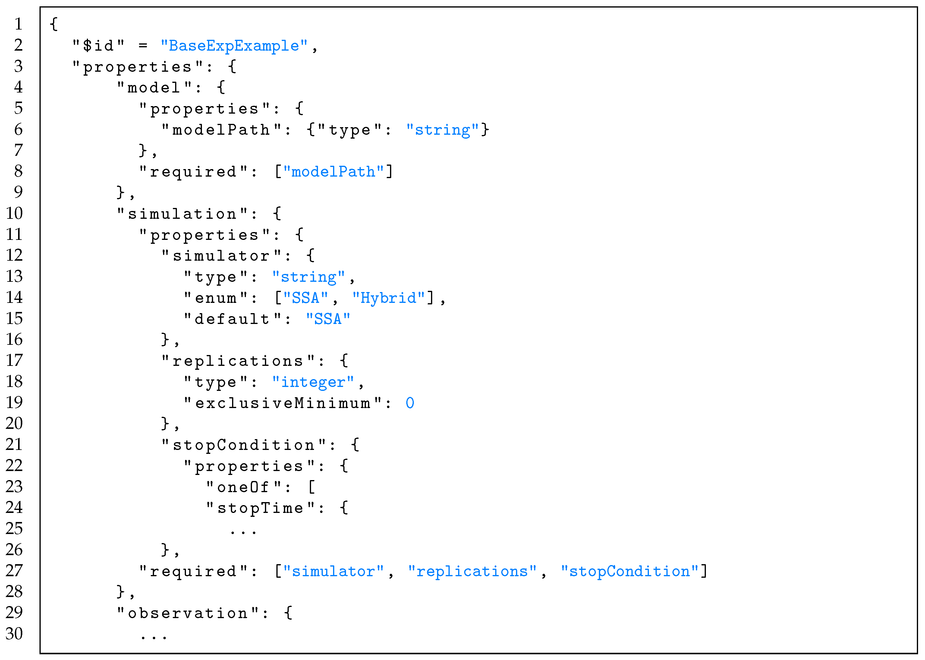
A base meta model for a fictive domain can be seen in
Listing 1 (meta models for experiment types can be created analogously). The meta model is defined using JSON Schema and contains all the necessary information in one, hierarchically structured file. It structures simulation experiments of the fictive domain into a model component, a simulation component, and an observation component. Each component encloses various other input properties, characterized by type, information, choices, default values, and constraints. For example, the constraint
exclusiveMinimum: 0 was added inside the property
replications. To express which inputs are required for specifying a valid simulation experiment, the keyword
required can be used. Furthermore, default values can be expressed explicitly, e.g., for setting the stochastic simulation algorithm (
SSA) as the standard simulator type of the domain. Moreover, to express alternatives, the keyword
oneOf is used, as in the case of
stopCondition, which can be given by (a) a specific stop time or (b) an expression on the model output. To build a valid simulation experiment that conforms to the meta model, exactly one of these alternatives needs to be applied. However, to keep the example short, we do not specify these options further and omit the details of the observation component.
For specifying a simulation experiment, at least a base meta model needs to be selected and filled with concrete input values by a user. However, the base meta models can also be flexibly composed with the various meta models for experiment types to create a meta model for the current experimentation task at hand. Using the composition mechanism, complex simulation experiments (such as statistical model checking, parameter estimation, steady state analysis, etc.) can be supported for any modeling approach or domain. This is possible due to the orthogonality of the base experiment specification and the experiment type specification. Note that in this paper, we focus on the main experiment types and their methods and do not discuss further analyses (i.e., post-processing or plotting of the results). However, this could be added as another component in the meta models. The language SED-ML [
9], for instance, allows the specification of various plot types including axis labels, etc.
3.4. Meta Model Repository
The meta models are developed based on external knowledge from domain experts and potential users and are stored in a meta model repository. This gives users (modelers) access to a variety of meta models that they can flexibly compose, as discussed earlier. The meta models may be developed by users on-demand to fit their use cases; however, we currently recommend that meta models be built by developers, i.e., persons with software engineering experience. For developers, the existing meta models contained in the repository can be the starting point for developing new ones. Often, depending on the needs of the new domain or approach, not everything has to be developed from scratch, but meta model components can be exchanged, added, or modified. Here, the reuse of knowledge about simulation experiments is not limited by specific domains and approaches. For example, research in the context of DES [
8,
42] and computational biology [
43] has identified a few common constituents of basic simulation experiment specifications: model configuration, simulation initialization, and observation. With respect to experiment types, meta models can be extended to include more elaborate methods, e.g., new sampling strategies or distance measures.
3.5. Interfaces
Our pipeline can be used in two ways. The first option is a dynamic GUI, which we provide with our framework. Depending on the selected base meta model and the experiment meta model, a tailored GUI is generated to support modelers in specifying their simulation experiments.
Figure 3 shows a screenshot of a GUI generated from the meta model example shown in
Listing 1 and a meta model for SA. In the GUI, the meta model components are displayed as individual tabs (“Model”, “Simulation”, “Observation”), input properties are displayed as rows, and alternative definitions are selected via drop-down menus, where, depending on the selection, other input properties become available as in the case of “Stop Condition”. The selection of the domain or approach and the experiment type takes place in the tab “Meta Model”. Thereby, an additional tab for the experiment type “Sensitivity Analysis” was created (
Figure 3). The tab “Backends” is used to select the code generation target.
As the second option, we provide a CLI. It allows flexible integration of our model-driven framework with other software. Via the CLI, the meta models can be selected and composed, the experiment inputs can be passed and validated, the GUI can be opened, the target backend can be chosen, and the experiment code can be generated or parsed. Consequently, one could integrate our framework with a procedure that automatically extracts certain experiment inputs from the model documentation (parameter tables or conceptual model) [
17,
18] or automatically generates simulation experiments from inside a workflow system (see
Section 5). If not all input fields dictated by the meta model can be filled automatically, the simulation experiment can be completed manually through the user interface.
3.6. Experiment Validation
Before inputs are passed on to the next layer (
) to produce a concrete tool-independent experiment specification, the entered values have to be validated. The validator checks conformance with the chosen meta models, and thus, both structural checks and type checks are carried out. After each validation cycle, the validator gives immediate feedback to the user (see
Figure 3) or the application, depending on which interface is used for the interaction. This step-by-step guidance supports inexperienced users, but also experienced users can benefit, as they do not have to concern themselves with the intricate details of simulation experiment specifications and, instead, can concentrate on important tasks such as output analysis and result interpretation.
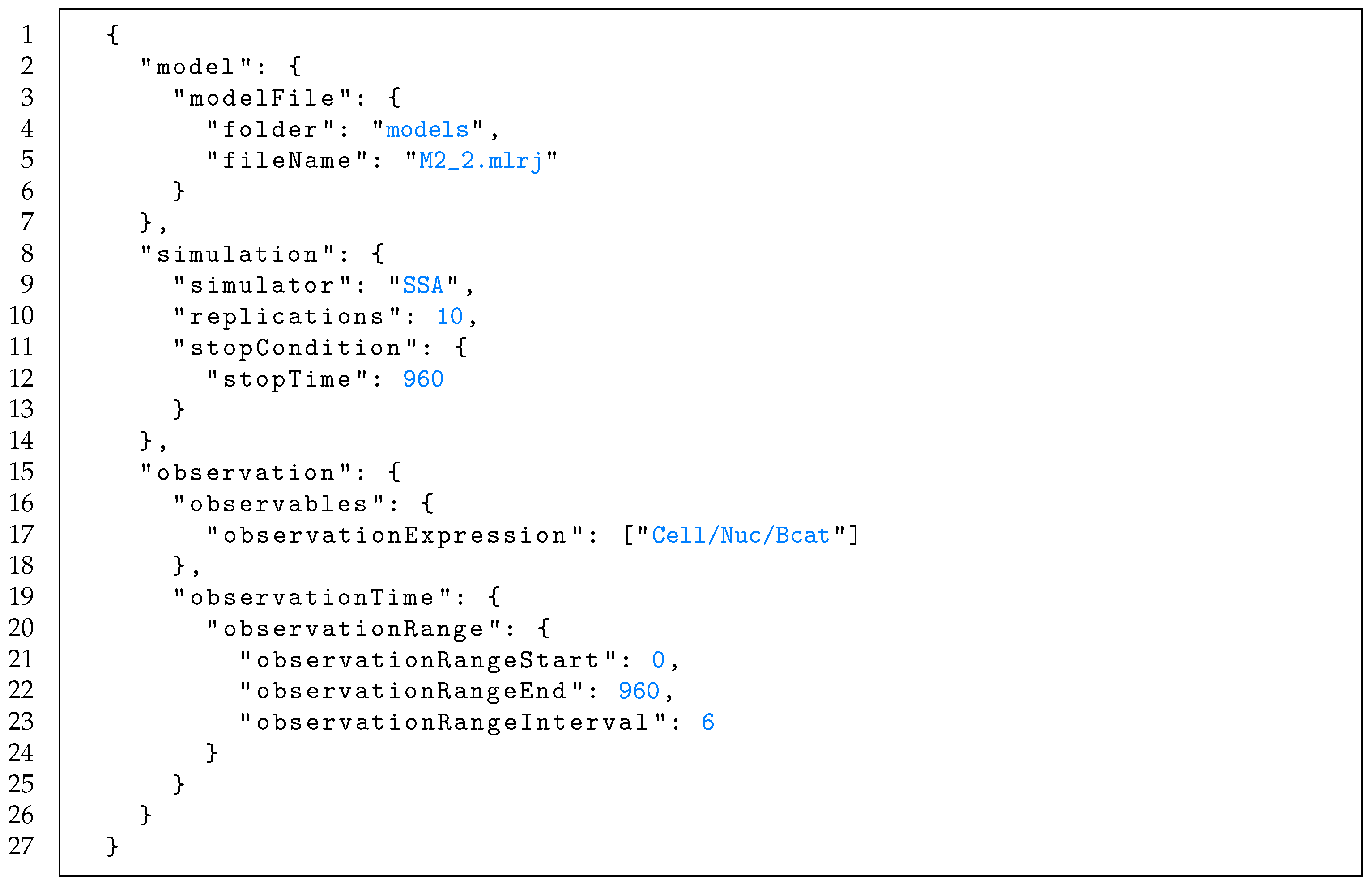
Listing 2 shows a created JSON document at the layer
. The document was validated according to the meta model example described above. The validation was unsuccessful due to the missing property
modelPath and due to using the wrong data type for the input property
replications.
3.7. Transformations and Bindings
The experiment meta models provide a general vocabulary that all modeling and simulation tools can refer to and communicate with. Meta models are therefore one way for improving the interoperability of modeling and simulation software. To go from an abstract experiment specification in a tool-independent format to executable code, the meta models have to be mapped to the syntax of actual modeling and simulation tools. During this transformation step, also differences in the terminology need to be resolved, e.g., the concept of the SSA has numerous implementations and is therefore known under different names such as the NextReactionMethod() or GibsonBruck() method.
Often, one wants to generate code for a single tool and, thus, in a single language. However, it is not uncommon to run the simulations in one tool, collect the results, and then, run the analysis in another. Our transformation mechanism supports the combination of tools for simulation and analysis and, thus, allows generating a combination of two scripts in two different languages. Moreover, for certain experiment types, such as SA, the toolchain can be divided further (see
Section 5.2).
Another important feature of the transformations is their bidirectionality. This means that we can (backward) parse a concrete experiment specification of a specific language and represent it in the canonical format. From there, forward transformations can generate the same experiment for a different tool, or the experiment may be reused and adapted for a different purpose.
Although it seems arduous to implement a transformation, it is far more efficient than connecting all pairs of tools individually. Moreover, once agreed upon in the community, the structure and vocabulary of a meta model are persistent and will rarely change, but rather be extended with new content, which will lead to some extensions in the transformations. It might also be beneficial to maintain transformations to distinct versions of the same M&S tool or to legacy systems for keeping older simulation experiments reproducible and, for example, for testing the tool itself. In addition, the experiment meta models provide guidelines for implementing new tools and, therefore, promote a more structured approach for developing modeling and simulation software.
In addition to the code transformations, we maintain so-called bindings to the various tools for which the code is generated. The bindings allow us to automatically start the generated experiments in the chosen backend. The backend and the implemented features within the backend then may allow the modeler further interventions, such as pausing simulation runs or interactively zooming into parameter ranges (e.g., using visual analytics). Note that a suitable backend could also be chosen automatically for a given task since the transformations make explicit which experimentation methods are implemented where.
4. Implementation
Our model-driven framework for conducting simulation experiments is realized in Java 8. This proof-of-concept implementation, thus far, comprises meta models for three simulation domains and different experiment types, the validation component, transformations and bindings to several backends, as well as the GUI and the CLI. The source code is publicly available in a Git repository (
https://git.informatik.uni-rostock.de/mosi/exp-generation, accessed on 26 July 2022).
At the heart of the implementation are the simulation experiment meta models, which are implemented using JSON Schema, Draft-07 [
40]. We selected JSON Schema as a basis to formulate our schemas, since over the past few years, JSON has probably become the most popular format for exchanging data on the web, and therefore, a variety of capable parsers and validators exist.
When launching the application, our dynamic GUI, implemented using JavaFX, is opened by default. After the user selects one of the included schemas, the GUI generates the necessary input tabs and fields (as shown in
Figure 3). When pressing the “Generate Experiment” button, all collected user inputs are stored in the multipurpose data interchange format JSON [
44] and presented to the user. The JSON files are validated against the JSON schemas using an open-source JSON Schema validator for Java, based on the org.json API [
45]. Thereafter, the experiment specification for the selected backend is generated.
For the mapping between the general schema inputs in JSON and the syntax of actual modeling and simulation tools, we used the template engine FreeMarker [
46]. FreeMarker has a built-in template language in which the mappings can be specified. For each backend and schema input property, a mini template is implemented. A master template joins all the template snippets together. The template engine takes this master template and fills the template variables with the data from the JSON file.
As an alternative to the GUI, we also provide a CLI, which allows for even more flexibility when working with our framework. For instance, one can transform an existing experiment specification for a target backend by running the command-line tool with the option -t <originalFile> <targetBackend>.
The backends and formats currently supported by our framework are SESSL/ML-Rules with R, SystemC-AMS with Python, the Python libraries EMStimTools and Uncertainpy, and SED-ML (see the Evaluation Section, where their application is described).
The time required for the experiment generation and transformation took less than a second on a standard laptop for the experiments shown in the evaluation. Thus, the execution time can be regarded as negligible in comparison to the time needed for experiment planning and input collection (which still have to be performed by the user and can only partly be automated). In fact, the overall time to create a simulation experiment may be decreased as the user is not bothered with the syntactical intricacies of the experiment types in the various specification languages and tools.
5. Evaluation
Applying MDE for simulation experiments has positive effects on the building and sharing of knowledge, the productivity and quality of code, the reusability, as well as the automatic generation of simulation experiments. This will ultimately lead to entire simulation studies being conducted in a more effective and systematic manner.
We demonstrate the benefits using three real simulation studies from the interdisciplinary research project ELAINE on electrically active implants. These comprise the DES study of a cell signaling pathway by Haack et al. [
47,
48], the virtual prototyping study of a neurostimulator by Heller et al. [
49], and the FEA study of electric fields in a stimulation chamber by Zimmermann et al. [
50]. We believe that well-designed and realistic case studies are the best way to convince modelers to adopt MDE for simulation experiments in their daily practice and to integrate this approach with other toolchains.
In the following, we first develop meta models to capture the characteristics of the three modeling and simulation approaches together with our domain modeling experts (stochastic DES, virtual prototyping, and FEA) and discuss how knowledge about simulation experiments can be exchanged within, but also between the different modeling and simulation communities. Next, we demonstrate that based on the base meta models composed with a shared meta model for the experiment type “global sensitivity analysis”, three complex simulation experiments can be specified in a straightforward manner to solve actual problems in the different application domains (analysis of a cell signaling pathway, the battery of a neurostimulator, and the electric field in a stimulation chamber). Then, we show how our JSON-based format can act as a standard exchange format to facilitate the automatic reuse of simulation experiments, e.g., for the cross-validation of two related cell signaling models. Finally, we show how our approach can be used to automatically generate simulation experiments by extracting information from a workflow.
Note that all the experiments we describe are only snapshots of the three studies in the form of single simulation experiments. During the simulation studies, of course, further analysis steps with the same or other experiment types (e.g., simulation-based optimization or statistical model checking) are involved, until the initial research questions can be answered. For these further steps, our approach can be applied analogously.
5.1. Improved Knowledge Sharing across Domains
The three simulation studies were conducted in the context of electrically active implants. However, they focused on different aspects involved in the development of such implants and, therefore, required different modeling and simulation approaches. Consequently, they required different meta models for the conducting of their basic experiments. In this section, we introduce meta models for these approaches, i.e., the base experiments for stochastic DES, virtual prototyping of heterogeneous systems, and FEA in electromagnetics. This demonstrates the versatility of our approach and—most importantly—its value for improving knowledge sharing within and across the diverse domains and approaches of modeling and simulation.
5.1.1. Meta Model for Stochastic Discrete-Event Simulation
Stochastic DES is applied for modeling systems where the variables change at discrete time points, and the time of the next event is determined stochastically [
51,
52]. In cell biology, e.g., modeling and simulating stochastic effects is of significant interest, especially for processes that involve low copy numbers [
53]. Stochastic DESs are also increasingly applied in demography [
54] or epidemiology [
55] as an alternative to the traditional discrete-time step simulation approach.
For the paper, we use tables to represent the meta models in a compact and readable way. The implementation as JSON Schema documents can be viewed in our source code.
Table 1 shows the developed DES meta model, which comprises three essential components, i.e., model configuration, simulation initialization, and observation (represented by sections in the table). In the meta model, each component of a simulation experiment requires specific inputs (table rows). For instance, typical ingredients for a stochastic simulation are now made explicit, such as the number of replications, the random seed, and the number of parallel threads (see the simulation component). Each input is characterized by a unique name, a description, a data type, a set of choices, a default value, and information about whether this input is required or optional (table columns). Properties of type Map (e.g.,
configuration) assemble related inputs as key–value pairs. The assembled sub-properties are indicated by “•”. Other properties (e.g.,
model,
stopCondition, or
observationTime) are of type
Alternative and provide different ways of specifying a property. The different options are indicated by “→”. For instance, the simulation model can be provided by either a folder and file name (local files) or a reference to an online resource.
The above meta model generalizes the structure and ingredients of the simulation experiments at the level of the modeling and simulation approach (i.e., DES). It can therefore be used for supporting the specification and execution of basic simulation experiments in various modeling domains, such as cell biology or digital circuits.
5.1.2. Meta Model for Virtual Prototyping of Heterogeneous Systems
Virtual prototyping allows for the design and development of products via modeling and simulation where building real prototypes is infeasible, e.g., due to ethical concerns or time restrictions, as in the case of neurostimulators for deep brain stimulation [
49]. The fundamental paradigm for modeling and simulation of digital circuits is DES. This means that the knowledge about the ingredients of simulation experiments captured in the DES meta model can be applied here as well. However, some virtual prototypes include components outside of the digital domain (e.g., to model the voltage levels of a battery) and, thus, require continuous-time representation. For these models, using the DES meta model for the simulation experiments does not suffice. However, using our framework, we can, with relatively low effort, define a new experiment meta model for virtual prototyping of heterogeneous systems (with mixed digital and analog signals) based on the existing DES experiment meta model. The model configuration component and the observation component can be reused from the shared meta model repository as they are. Only the simulation initialization component needs to be adapted for the new simulation approach (see
Table 2). The main difference is that, now, a fixed time step and time step unit are included, at which the discrete-time and continuous-time models are synchronized. Furthermore, the modified meta model does not include the type of solver or scheduler explicitly, as this is usually assigned automatically to specific semantics defined in the language standard (e.g., SystemC-AMS [
56]). Thus, the solver or scheduler is part of the simulation model and not changed in the experiments.
5.1.3. Meta Model for Finite Element Analysis in Electromagnetics
FEA is a general method that is capable of treating complex geometries and accurately computing, e.g., the properties and effects of electric fields in deep brain stimulation. A partial differential equation describing electric fields in the frequency domain is solved (physical model). Thus, time–harmonic fields are described and only the quasi-static behavior of the system under investigation is considered. The 3D geometry of the system is modeled explicitly, and corresponding boundary conditions and material properties are directly linked to the different domains of the geometric model. As FEA is a completely different modeling and simulation approach, no parts from the previously defined base meta models can be reused, and a new one is developed. Due to the separation of the geometric model and physical model, the experiment meta model for FEA (see the
Supplementary Material, Table S1) has two new components: geometric model and physical model. These are complemented by a simulation component that comprises information about the type of solver and the accuracy of the solution (given by the coarseness of the mesh). For the observation component, derived quantities can be specified, as well as coordinates at which to evaluate these quantities.
Note that this first draft of the FEA experiment meta model was developed with the background of electromagnetics in mind. Future efforts should aim to support FEA more generally. In particular, the various inputs and constraints depending on the type of physics need to be identified. In addition, multiphysics applications where mechanics, electromagnetics, and thermodynamics are coupled are of potential interest. In each discipline, PDEs comprising material properties together with geometrical constraints are the basis of the modeling approach [
57]. Hence, the current meta model can provide a basis for further discussions and adjustments.
5.2. Increasing Productivity and Quality for Complex Experiments
Besides sharing information about the base experiments, our approach is designed to share meta models for diverse, complex experiment types.
Table 3, for instance, shows a meta model for global SA, which could be added to any of the above-described base meta models. It comprises various important ingredients for the specification of global SAs, such as factor ranges and factor distributions, as well as a choice of different sampling strategies: Monte Carlo (
MC) and quasi-Monte Carlo (
QMC) [
58], orthogonal Latin hypercube (
OLHC) [
59], and polynomial chaos expansion (
PC) [
60]. For the first three strategies, the samples are used directly to calculate the indices. With a PC, on the other hand, first, a surrogate model is constructed based on which indices are computed. As the index type, e.g., Sobol indices [
61,
62] can be used, which are variance-based measures. The first-order Sobol index of factor
describes the individual contribution of this factor to the overall variance in the output
:
The total-order sensitivity index,
, accounts for all the contributions to the output variation due to factor
(i.e., first-order index plus higher-order interactions):
Having made explicit the ingredients of global SA as a meta model, we can easily specify simulation experiments to calculate Sobol indices for various simulation models. We show this for three different models by composing the respective base meta model with the SA meta model. This has the potential to increase productivity during the simulation study since guidance is provided via a specialized GUI or CLI and input validation. Moreover, the complicated details of the code are abstracted away by the model-driven approach. Thus, the modeler does not have to worry about how to combine the simulation tools and analysis tools in a complex experiment.
Figure 4 shows three different ways of performing a Sobol analysis; they all can be generated using the same meta model.
5.2.1. Sensitivity Analysis of a Wnt Signaling Model
To understand how electrically active implants affect the differentiation and proliferation of cells (and, thus, the composition and regeneration of tissue), the impact of external electric fields on central cellular signaling pathways needs to be studied. The Wnt/β-catenin signaling pathway is one of the central pathways that regulate the proliferation, as well as differentiation of cells [
63]. Deregulated forms of this pathway are involved in several human cancers and developmental disorders [
64]. Effects on membrane-related dynamics are of particular interest for the development of electrically active implants. Lipid rafts, specialized microdomains of the membrane, have been found to sense the electric field and to direct the responses of cells [
65]. Therefore, in the simulation study by Haack et al., a Wnt simulation model [
48] was extended to capture both raft- and non-raft-associated endocytic processes of the Wnt/β-catenin receptor LRP6 in detail, including stochastic effects [
47].
The model was written in ML-Rules [
66] and simulated using stochastic DES (the Wnt model, the SA experiment, and the analysis results are available at
https://github.com/SFB-ELAINE/Case-Study-Endocytosis, accessed on 26 July 2022). The experiment meta model for DES is available in the repository of the framework and can therefore be used to guide the modeler through the specification of the base experiment. Similarly, the meta model for global sensitivity analysis is available to guide the modeler through the definition of the global SA. In the global SA, the modeler is interested in the sensitivity of the fraction of the cell membrane receptor LRP6 (observed quantity), with regard to the model parameters
and
, which represent the internalization rates of bound LRP6 receptor complexes and the parameter
. Furthermore, the modeler specifies uniform distributions for these three factors, as well as minimum and maximum values and enters the information via the generated GUI for this experiment type. As the sampling strategy, an OLHC design with 1750 samples was selected.
Once all inputs for the SA have been collected, executable experiment code can be generated, i.e., a combination of an R script with an SESSL/ML-Rules script, as illustrated in
Figure 4A. Without the experiment generation, the user would have had required expertise in writing both SESSL/ML-Rules scripts and R scripts, as well as expertise in the types of sensitivity analyses and the respective libraries. Especially for novice modelers, correctly setting up a sensitivity analysis involving two specification languages can be challenging and error-prone, and therefore, quality and productivity can be improved by the MDE approach.
Since we have implemented bindings to both SESSL/ML-Rules and R, the composed experiment can also be executed automatically. Note that, for now, we do not support the automatic analysis of simulation results and the generation of plots; however, this could be included as a feature of this framework in the future.
Figure 5A presents the results of the experiment to be interpreted by the user. They show almost no impact of the parameter
on the results. The variances of each of the other two parameters (
and
) make up about half of the variance of the result.
5.2.2. Sensitivity Analysis of a Battery Model
Deep brain stimulation is a therapy option for a multitude of neurological disorders. While it is widely implemented in the clinical routine, especially for Parkinson’s disease and dystonia, the underlying mechanisms are not fully understood. Since most experiments cannot be performed directly on humans due to ethical reasons, animal testings are necessary. However, rodent-specific implants require a highly optimized level of miniaturization and power consumption compared to human implants. Physical prototyping is not feasible as the pursued runtime is more than a year. Therefore, virtual prototyping is used to design neurostimulators for rodents. The model by Heller et al. [
49] considers the interplay between various heterogeneous system components (i.e., battery, boost converter, microcontroller, and stimulation unit) and, thus, combines digital, as well as analog components. Whereas previous studies focused on the optimization of voltage levels inside the system, this study focuses on understanding the implications of different battery parameters on the overall runtime of the implant. The described SA experiment and the analysis results are available at
https://github.com/SFB-ELAINE/Case-Study-Neurostimulator (accessed on 26 July 2022). Unfortunately, the battery model itself cannot be provided, as it is part of a closed-source project.
As they vary over different battery types, the internal resistance
Ri, the battery capacity
Q, and the polarization constant
K are of special interest. To facilitate the analysis of these parameters, the modeler uses the model-driven framework and selects the meta model for global SA (
Table 3) to enhance an already specified base experiment. Parameter ranges and Gaussian distributions are requested for the three factors and entered by the user, and a QMC sampling is selected with 1000 samples. A schematic of the generated code, based on the Python package Uncertainpy [
67] and SystemC-AMS [
56], is shown in
Figure 4B. The generated experiment was started automatically; however, due to the complexity of the model, even after 12 h, the analysis did not converge. Therefore, the experiment was terminated by the user to find a more efficient approach. With the assistance of the model-driven framework, the sampling strategy could easily be substituted by PC as the meta model for global SA provides a number of different sampling strategies to choose from and automatically accounts for additional inputs or constraints associated with this other method. Overall, the MDE framework allows the user to quickly try out and compare different methods, e.g., also different sensitivity indices might be compared in the same way.
Using a PC, the described experiment was automatically repeated and the runtime could be reduced to less than 3 h. The SA results, visualized by the user, are depicted in
Figure 5B and show that the model response is strongly determined by interactions between the parameters. The internal resistance seems to have a particularly strong effect on the overall battery runtime. Consequently, one should aim for measuring this parameter in (real) experiments and pre-select batteries with lower internal resistance.
5.2.3. Sensitivity Analysis of an Electric Fields Model
The third simulation study aims to compute the electric field distribution in a specific chamber [
50]. Based on the computed field distributions, the biological response of the stimulated biological sample can be linked to certain specifications of the electrical stimulation setup. A global SA was used to evaluate the influence of the dielectric parameters on the electric field strength at specific locations of the cells (the model, the described SA experiment, and the analysis results are available at
https://github.com/j-zimmermann/EMStimTools/tree/master/examples/experimentSchemas (accessed on 26 July 2022)).
Following the structure of the meta model, the modeler enters all the required information into the GUI (i.e., various material properties as factors and their value ranges) and assumes uniform distributions. A PC was chosen as the sampling method, as it is an often applied method in FEA, where simulation runs are computationally expensive.
Figure 4C shows the generated code, which combines the Python package EMStimTools [
68] with Uncertainpy [
67]. Again, the structured approach of this framework allows the user to quickly specify and execute the desired simulation experiment, even without prior knowledge of the Uncertainpy package.
The first- and total-order Sobol indices are shown in
Figure 5C. The results suggest that a change in the permittivity of the medium does not influence the field strength. Hence, the user concluded that the permittivity can be neglected in future uncertainty analyses for this kind of problem and similar input parameters.
5.3. Reusability
The final Wnt model (introduced in
Section 5.2.1) is the result of successively extending simpler model versions. The original Wnt model by Lee et al. (2003) [
69] was extended by raft- and redox-dependent signaling events in a study by Haack et al. (2015) [
48]. This new model was then extended further by endocytic processes in Haack et al. (2020) [
47]. To ensure that the basic model behavior was not changed due to the extensions, various cross-validation experiments were required that compared the trajectories of the variables of interest.
Therefore, the original simulation experiments of the study by Lee et al. shall be reused and repeated with the extended model. However, the original experiments were specified in SED-ML [
9] and the corresponding model in SBML [
70] (see BioModels [
71] entry at
https://www.ebi.ac.uk/biomodels/BIOMD0000000658, accessed on 26 July 2022). In contrast, the Wnt model by Haack et al. (2015/2020) was specified using the rule-based modeling language ML-Rules [
66], and the experiments were conducted using the experiment specification language SESSL [
8]. Thus, in order to reproduce results from the study by Lee et al., the SED-ML experiment specification needs to be adapted for the new model and translated to SESSL. This can be supported by the model-driven approach.
First, the meta model for DES directs the automatic parsing of the original specification and provides meaning to the parts of the experiment specification. As the experiment type is a time course analysis, a base meta model suffices to capture all the inputs. Once transformed to the quasi-standardized JSON format, the experiment specification can be adapted to work with the model by Haack et al., e.g., the file name and the simulation stop time (due to the use of different time scales) need to be changed. This can partly be performed automatically by exploiting additional knowledge in the form of ontologies, e.g., UniProt [
72] provides a unique identifier for each protein and allows transforming the variable names in the observation expressions from one model to another. Especially, these ontology-based automatic transformations are valuable for the reuse of simulation experiments as they prevent inconsistencies that can easily happen when translating an experiment for a different model or a different specification language. As mentioned, the variable names might have a different meaning in Model A compared to Model B, but also, e.g., the units used for the rate constants might differ. Incorrect translations may lead to distorted simulation results and, therefore, seemingly different model behavior, leading to the wrong conclusion that the new model cannot be successfully cross-validated.
The automatically parsed and transformed experiment specification is then presented to the user to ask for adaptions or additional information that could not be extracted from the old specification.
Listing 3 shows the finished experiment specification in the JSON-based exchange format after being adapted for the model by Haack et al. From this, the SESSL-specific experiment can be generated and executed automatically.
The result of the cross-validation is depicted in
Figure 6. It compares the trajectories of the key protein β-catenin, an indicator of the pathway’s activity, produced by the Lee et al. and the Haack et al. model (with an adapted time scale) when stimulated with a transient Wnt stimulus. Both β-catenin curves show the same peak at the same time. From this, the user concludes that the extensions applied in the study by Haack et al. do not alter the central dynamics of the pathway.
5.4. Automation
In the previous subsection, we already saw one case of automation, i.e., we demonstrated that a well-designed MDE pipeline is the foundation for reusing simulation experiments automatically [
19] and allows integrating with ontologies. Now, we go one step further and show that we can integrate this approach with other frameworks for supporting simulation studies as a whole, e.g., an artifact-based workflow (an IDE for simulation studies).
In an artifact-based workflow, the central products of simulation studies are identified and made explicit as artifacts. These include the conceptual model, the simulation models, and the simulation experiments. Each artifact is characterized by stages a modeler can move through to achieve certain milestones and preconditions called guards [
4].
Figure 7 shows the conceptual model artifact of an artifact-based workflow for FEA studies [
73]. While moving through the stages of the conceptual model, the modeler specifies various meta-information about the model, such as the modeling objective, requirements, and input data, which are stored inside the artifact. This meta-information of the conceptual model artifact, as well as other artifacts, can be used in the automatic generation of simulation experiments. For instance, in [
73], an FEA simulation study of an electrical stimulation chamber was conducted with assistance from the workflow. Once the user reaches the stage
Specifying simulation experiment, the MDE-based experiment generation can be triggered. For instance, the information collected by the workflow could be used to automatically generate a convergence test for the model. The convergence of numerical methods is of high importance in order to retrieve meaningful results from a numerical simulation [
74]. In a convergence experiment, the mesh is incrementally refined until the estimated discretization error lies below a given error threshold or until the maximum number of iterations is reached. A meta model for convergence experiments, therefore, requires the following inputs:
The region of interest;
An error metric allowing to estimate the discretization error for a given region;
The maximum number of iterations or an error threshold to control the error;
An initial meshing hypothesis, i.e., the minimum and maximum size of the finite elements, to initialize the meshing algorithm.
By connecting our command-line tool to the workflow system, some of these inputs required by the meta model can be filled automatically by extracting meta information from the artifacts, e.g., the region of interest and the error metric were specified as requirements in the conceptual model [
4]. Other inputs are specific to convergence studies, e.g., the initial minimum and maximum size of the elements, and thus, either need to be entered manually by the user (e.g., by opening our GUI pre-filled with the extracted values) or are initialized with default values (specified in the experiment meta model).
Figure 8 shows the results of the convergence experiment that was generated semi-automatically for the model of the electrical stimulation chamber. It shows how the observed variable (current at Electrode 1) converges with increasing degrees of freedom in the finite element model and that the refinement could terminate after the fourth iteration.
6. Conclusions
In this paper, we presented an MDE framework for supporting the conducting of simulation experiments. Central features of the approach are the composition of different types of meta models, a meta model repository, bidirectional code transformations, a variety of tool bindings, and a GUI, as well as a CLI.
We demonstrated how the framework contributes to improving knowledge structuring and sharing within, but also across the different simulation domains and approaches (i.e., stochastic DES of a cell signaling pathway, virtual prototyping of a neurostimulator, and FEA of electric fields). There, the introduction of meta models for base experiments and meta models for complex experiment types proved crucial. Their on-demand composition guided the modeler in specifying complex experiments (SA) while catering to rather diverse demands of the respective simulation studies and, thus, raises the productivity of the modeler and the quality of complex experiments. Furthermore, we showed the framework’s practicality for automatically reusing simulation experiments for the cross-validation of related models and for automatically generating and executing simulation experiments, e.g., for conducting convergence tests initiated by a workflow system. We showed that the presented approach fulfills the typical expectations and advantages associated with MDE and will be an asset for more effective and systematic simulation studies. The user only needs to fill in the information required by the respective meta models, obviating the need to manually write experiment code and acquire expertise in heterogeneous tools and experiment specification languages. Thereby, the approach holds the promise to reduce the effort of conducting simulation experiments and to increase the accessibility of various types of simulation experiments.
For future work, we plan to extend support for the development of new meta models of base experiments and meta models of complex experiment types, i.e., through the composition and reuse of meta model parts with a clear notion of inheritance. What should become part of a meta model needs to be debated in the various modeling and simulation communities, possibly via standardization bodies such as SISO [
75]. Regarding the automation of simulation studies, we plan to build further support components on top of the MDE pipeline, such as an automatic selection and parametrization of experiment types and methods.
Supplementary Materials
The following are available online at
https://www.mdpi.com/article/10.3390/app12167977/s1, Table S1: Base meta model for conducting simulation experiments in finite element analysis. A geometric model, a physical model, and a solver need to be provided and configured. Optionally, observations and derived properties can be specified. The rows describe the different input properties of the meta model. Sub-properties are denoted by “•”. Alternative meta model parts are indicated by “→”.
Author Contributions
Conceptualization, P.W. and A.M.U.; data curation, P.W., J.H., K.B. and J.Z.; funding acquisition, C.H., D.T., U.v.R. and A.M.U.; investigation, J.H., K.B. and J.Z.; methodology, P.W. and T.W.; project administration, A.M.U.; software, P.W.; supervision, C.H., D.T., U.v.R. and A.M.U.; validation, P.W.; visualization, J.H., K.B. and J.Z.; writing—original draft, P.W. and A.M.U.; writing—review and editing, P.W., J.H., K.B., J.Z., T.W., C.H., U.v.R. and A.M.U. All authors have read and agreed to the published version of the manuscript.
Funding
This work was funded by the DFG (German Research Foundation) research project UH 66/18 GrEASE and the DFG Collaborative Research Center 1270/1 - 299150580 ELAINE.
Data Availability Statement
Acknowledgments
The authors would like to thank Fiete Haack for his excellent support in conducting the Wnt experiments.
Conflicts of Interest
The authors declare no conflict of interest. The funders had no role in the design of the study; in the collection, analyses, or interpretation of data; in the writing of the manuscript, or in the decision to publish the results.
References
- Winsberg, E. Science in the Age of Computer Simulation; University of Chicago Press: Chicago, IL, USA, 2010. [Google Scholar]
- Balci, O. A life cycle for modeling and simulation. Simulation 2012, 88, 870–883. [Google Scholar] [CrossRef]
- Sargent, R.G. Verification and validation of simulation models. J. Simul. 2013, 7, 12–24. [Google Scholar] [CrossRef] [Green Version]
- Ruscheinski, A.; Warnke, T.; Uhrmacher, A.M. Artifact-Based Workflows for Supporting Simulation Studies. IEEE Trans. Knowl. Data Eng. 2020, 32, 1064–1078. [Google Scholar] [CrossRef]
- Saltelli, A.; Aleksankina, K.; Becker, W.; Fennell, P.; Ferretti, F.; Holst, N.; Li, S.; Wu, Q. Why so Many Published Sensitivity Analyses Are False: A Systematic Review of Sensitivity Analysis Practices. Environ. Model. Softw. 2019, 114, 29–39. [Google Scholar] [CrossRef]
- Hinsch, M.; Bijak, J.; Hilton, J. Towards More Realistic Models. In Towards Bayesian Model-Based Demography: Agency, Complexity and Uncertainty in Migration Studies; Bijak, J., Ed.; Methodos Series; Springer International Publishing: Cham, Switzerland, 2022; pp. 137–154. [Google Scholar] [CrossRef]
- Prike, T. Open Science, Replicability, and Transparency in Modelling. In Towards Bayesian Model-Based Demography: Agency, Complexity and Uncertainty in Migration Studies; Bijak, J., Ed.; Methodos Series; Springer International Publishing: Cham, Switzerland, 2022; pp. 175–183. [Google Scholar] [CrossRef]
- Ewald, R.; Uhrmacher, A.M. SESSL: A Domain-specific Language for Simulation Experiments. ACM Trans. Model. Comput. Simul. 2014, 24, 1–25. [Google Scholar] [CrossRef]
- Waltemath, D.; Adams, R.; Bergmann, F.T.; Hucka, M.; Kolpakov, F.; Miller, A.K.; Moraru, I.I.; Nickerson, D.; Sahle, S.; Snoep, J.L.; et al. Reproducible computational biology experiments with SED-ML—The simulation experiment description markup language. BMC Syst. Biol. 2011, 5, 198. [Google Scholar] [CrossRef] [PubMed] [Green Version]
- Erdemir, A.; Guess, T.M.; Halloran, J.; Tadepalli, S.C.; Morrison, T.M. Considerations for reporting finite element analysis studies in biomechanics. J. Biomech. 2012, 45, 625–633. [Google Scholar] [CrossRef] [Green Version]
- Perrone, L.F.; Main, C.S.; Ward, B.C. SAFE: Simulation automation framework for experiments. In Proceedings of the 2012 Winter Simulation Conference (WSC), Berlin, Germany, 9–12 December 2012; pp. 1–12. [Google Scholar] [CrossRef] [Green Version]
- Sanchez, S.M.; Sánchez, P.J.; Wan, H. Work smarter, not harder: A tutorial on designing and conducting simulation experiments. In Proceedings of the 2018 Winter Simulation Conference (WSC), Gothenburg, Sweden, 9–12 December 2018; pp. 237–251. [Google Scholar] [CrossRef]
- Teran-Somohano, A.; Smith, A.E.; Ledet, J.; Yilmaz, L.; Oğuztüzün, H. A model-driven engineering approach to simulation experiment design and execution. In Proceedings of the 2015 Winter Simulation Conference (WSC), Huntington Beach, CA, USA, 6–9 December 2015; pp. 2632–2643. [Google Scholar] [CrossRef]
- Yilmaz, L.; Chakladar, S.; Doud, K. The Goal-Hypothesis-Experiment framework: A generative cognitive domain architecture for simulation experiment management. In Proceedings of the 2016 Winter Simulation Conference (WSC), Washington, DC, USA, 11–14 December 2016; pp. 1001–1012. [Google Scholar] [CrossRef]
- Mohagheghi, P.; Dehlen, V. Where is the proof?-A review of experiences from applying mde in industry. In European Conference on Model Driven Architecture—Foundations and Applications; Springer: Berlin/Heidelberg, Germany, 2008; pp. 432–443. [Google Scholar] [CrossRef] [Green Version]
- Robinson, S. Conceptual modelling for simulation Part I: Definition and requirements. J. Oper. Res. Soc. 2008, 59, 278–290. [Google Scholar] [CrossRef] [Green Version]
- Wilsdorf, P.; Haack, F.; Budde, K.; Ruscheinski, A.; Uhrmacher, A.M. Conducting Systematic, Partly Automated Simulation Studies—Unde Venis et Quo Vadis. In Proceedings of the 17th International Conference of Numerical Analysis and Applied Mathematics, Rhodes, Greece, 17–23 September 2020. [Google Scholar] [CrossRef]
- Ruscheinski, A.; Budde, K.; Warnke, T.; Wilsdorf, P.; Hiller, B.C.; Dombrowsky, M.; Uhrmacher, A.M. Generating Simulation Experiments based on Model Documentations and Templates. In Proceedings of the 2018 Winter Simulation Conference (WSC), Gothenburg, Sweden, 9–12 December 2018; pp. 715–726. [Google Scholar] [CrossRef]
- Wilsdorf, P.; Wolpers, A.; Hilton, J.; Haack, F.; Uhrmacher, A.M. Automatic Reuse, Adaption, and Execution of Simulation Experiments via Provenance Patterns. arXiv 2021, arXiv:2109.06776. [Google Scholar]
- Cetinkaya, D.; Verbraeck, A. Metamodeling and model transformations in modeling and simulation. In Proceedings of the 2011 Winter Simulation Conference (WSC), Phoenix, AZ, USA, 11–14 December 2011; pp. 3043–3053. [Google Scholar] [CrossRef]
- Guizzardi, G.; Wagner, G. Conceptual simulation modeling with Onto-UML advanced tutorial. In Proceedings of the 2012 Winter Simulation Conference (WSC), Berlin, Germany, 9–12 December 2012; pp. 1–15. [Google Scholar] [CrossRef]
- Santos, F.; Nunes, I.; Bazzan, A.L. Quantitatively assessing the benefits of model-driven development in agent-based modeling and simulation. Simul. Model. Pract. Theory 2020, 104, 102126. [Google Scholar] [CrossRef]
- Capocchi, L.; Santucci, J.F.; Pawletta, T.; Folkerts, H.; Zeigler, B.P. Discrete-Event Simulation Model Generation based on Activity Metrics. Simul. Model. Pract. Theory 2020, 103, 102122. [Google Scholar] [CrossRef]
- Bocciarelli, P.; D’Ambrogio, A.; Falcone, A.; Garro, A.; Giglio, A. A model-driven approach to enable the simulation of complex systems on distributed architectures. Simulation 2019, 95, 1185–1211. [Google Scholar] [CrossRef]
- Vangheluwe, H.; de Lara, J. Meta-Models are models too. In Proceedings of the Winter Simulation Conference, San Diego, CA, USA, 8–11 December 2002; Volume 1, pp. 597–605. [Google Scholar] [CrossRef]
- Dayıbaş, O.; Oğuztüzün, H.; Yılmaz, L. On the use of model-driven engineering principles for the management of simulation experiments. J. Simul. 2019, 13, 83–95. [Google Scholar] [CrossRef]
- Lorig, F. Hypothesis-Driven Simulation Studies; Springer: Wiesbaden, Germany, 2019. [Google Scholar] [CrossRef]
- Peng, D.; Warnke, T.; Haack, F.; Uhrmacher, A.M. Reusing simulation experiment specifications in developing models by successive composition—A case study of the Wnt/β-catenin signaling pathway. Simulation 2017, 93, 659–677. [Google Scholar] [CrossRef] [Green Version]
- Peng, D.; Warnke, T.; Haack, F.; Uhrmacher, A.M. Reusing simulation experiment specifications to support developing models by successive extension. Simul. Model. Pract. Theory 2016, 68, 33–53. [Google Scholar] [CrossRef]
- Cooper, J.; Scharm, M.; Mirams, G.R. The Cardiac Electrophysiology Web Lab. Biophys. J. 2016, 110, 292–300. [Google Scholar] [CrossRef] [Green Version]
- Wilsdorf, P.; Zimmermann, J.; Dombrowsky, M.; van Rienen, U.; Uhrmacher, A.M. Simulation Experiment Schemas—Beyond Tools and Simulation Approaches. In Proceedings of the 2019 Winter Simulation Conference (WSC), National Harbor, MD, USA, 8–11 December 2019; pp. 2783–2794. [Google Scholar] [CrossRef]
- Fishwick, P.A.; Miller, J.A. Ontologies for modeling and simulation: Issues and approaches. In Proceedings of the 2004 Winter Simulation Conference (WSC), Washington, DC, USA, 5–8 December 2004; p. 264. [Google Scholar] [CrossRef]
- Taylor, S.J.; Bell, D.; Mustafee, N.; de Cesare, S.; Lycett, M.; Fishwick, P.A. Semantic Web Services for Simulation Component Reuse and Interoperability: An Ontology Approach. In Organizational Advancements through Enterprise Information Systems: Emerging Applications and Developments; IGI Global: Hershey, PA, USA, 2010. [Google Scholar] [CrossRef]
- Silver, G.A.; Miller, J.A.; Hybinette, M.; Baramidze, G.; York, W.S. DeMO: An Ontology for Discrete-event Modeling and Simulation. Simulation 2011, 87, 747–773. [Google Scholar] [CrossRef] [Green Version]
- Cheong, H.; Butscher, A. Physics-based simulation ontology: An ontology to support modelling and reuse of data for physics-based simulation. J. Eng. Des. 2019, 30, 655–687. [Google Scholar] [CrossRef]
- Whittle, J.; Hutchinson, J.; Rouncefield, M. The State of Practice in Model-Driven Engineering. IEEE Softw. 2014, 31, 79–85. [Google Scholar] [CrossRef] [Green Version]
- Bezivin, J.; Gerbe, O. Towards a precise definition of the OMG/MDA framework. In Proceedings of the 16th Annual International Conference on Automated Software Engineering (ASE 2001), San Diego, CA, USA, 26–29 November 2001; pp. 273–280. [Google Scholar] [CrossRef]
- Unified Modeling Language. 2020. Available online: https://www.omg.org/spec/UML (accessed on 26 July 2022).
- Fallside, D.C.; Walmsley, P. XML schema part 0: Primer second edition. W3C Recomm. 2004, 16. Available online: https://www.w3.org/TR/xmlschema-0 (accessed on 26 July 2022).
- JSON Schema Specification. 2019. Available online: https://json-schema.org/draft/2019-09/release-notes.html (accessed on 26 July 2022).
- Object Constraint Language, 2020. Available online: https://www.omg.org/spec/OCL/About-OCL (accessed on 26 July 2022).
- Zeigler, B.P. Multifacetted Modelling and Discrete Event Simulation; Academic Press Professional, Inc.: San Diego, CA, USA, 1984. [Google Scholar]
- Waltemath, D.; Adams, R.; Beard, D.A.; Bergmann, F.T.; Bhalla, U.S.; Britten, R.; Chelliah, V.; Cooling, M.T.; Cooper, J.; Crampin, E.J.; et al. Minimum Information About a Simulation Experiment (MIASE). PLoS Comput. Biol. 2011, 7, e1001122. [Google Scholar] [CrossRef] [PubMed]
- Introduction to JSON, 2020. Available online: http://www.json.org (accessed on 26 July 2022).
- JSON Schema Validator, 2020. Available online: https://github.com/everit-org/json-schema (accessed on 26 July 2022).
- Apache FreeMarker Manual for Freemarker 2.3.30. 2020. Available online: https://freemarker.apache.org/docs/index.html (accessed on 26 July 2022).
- Haack, F.; Budde, K.; Uhrmacher, A.M. Exploring mechanistic and temporal regulation of LRP6 endocytosis in canonical Wnt signaling. J. Cell Sci. 2020, 133, jcs243675. [Google Scholar] [CrossRef] [PubMed]
- Haack, F.; Lemcke, H.; Ewald, R.; Rharass, T.; Uhrmacher, A.M. Spatio-temporal Model of Endogenous ROS and Raft-Dependent WNT/Beta-Catenin Signaling Driving Cell Fate Commitment in Human Neural Progenitor Cells. PLoS Comput. Biol. 2015, 11, e1004106. [Google Scholar] [CrossRef] [Green Version]
- Heller, J.; Christoph, N.; Plocksties, F.; Haubelt, C.; Timmermann, D. Towards Virtual Prototyping of Electrically Active Implants Using SystemC-AMS. In Proceedings of the Workshop Methods and Description Languages for Modelling and Verification of Circuits and Systems (MBMV), Stuttgart, Germany, 19–20 March 2020; pp. 29–36. [Google Scholar]
- Zimmermann, J.; Budde, K.; Arbeiter, N.; Molina, F.; Storch, A.; Uhrmacher, A.M.; van Rienen, U. Using a digital twin of an electrical stimulation device to monitor and control the electrical stimulation of cells in vitro. Front. Bioeng. Biotechnol. 2021, 9. [Google Scholar] [CrossRef]
- Law, A.M.; Kelton, W.D. Simulation Modeling and Analysis; McGraw-Hill: New York, NY, USA, 2000; Volume 3. [Google Scholar]
- Banks, J.; Carson, J.S.; Nelson, B.L.; Nicol, D.M. Discrete-Event System Simulation, 5th ed.; Prentice Hall: Hoboken, NJ, USA, 2010. [Google Scholar]
- Székely, T., Jr.; Burrage, K. Stochastic simulation in systems biology. Comput. Struct. Biotechnol. J. 2014, 12, 14–25. [Google Scholar] [CrossRef] [PubMed]
- Warnke, T.; Reinhardt, O.; Klabunde, A.; Willekens, F.; Uhrmacher, A.M. Modelling and simulating decision processes of linked lives: An approach based on concurrent processes and stochastic race. Popul. Stud. (Camb.) 2017, 71, 69–83. [Google Scholar] [CrossRef] [PubMed] [Green Version]
- Cauchemez, S.; Ferguson, N.M. Likelihood-based estimation of continuous-time epidemic models from time-series data: Application to measles transmission in London. J. R. Soc. Interface 2008, 5, 885–897. [Google Scholar] [CrossRef] [PubMed] [Green Version]
- Vachoux, A.; Grimm, C.; Einwich, K. Analog and mixed signal modelling with SystemC-AMS. In Proceedings of the 2003 International Symposium on Circuits and Systems (ISCAS), Bangkok, Thailand, 25–28 May 2003; Volume 3, p. III. [Google Scholar] [CrossRef] [Green Version]
- Logg, A.; Mardall, K.A.; Wells, G.N. Automated Solution of Differential Equations by the Finite Element Method; Springer Science & Business Media: Berlin/Heidelberg, Germany, 2012. [Google Scholar] [CrossRef]
- Caflisch, R.E. Monte carlo and quasi-monte carlo methods. Acta Numer. 1998, 1998, 1–49. [Google Scholar] [CrossRef] [Green Version]
- Butler, N.A. Optimal and orthogonal Latin hypercube designs for computer experiments. Biometrika 2001, 88, 847–857. [Google Scholar] [CrossRef]
- Crestaux, T.; Le Maıtre, O.; Martinez, J.M. Polynomial chaos expansion for sensitivity analysis. Reliab. Eng. Syst. Saf. 2009, 94, 1161–1172. [Google Scholar] [CrossRef]
- Homma, T.; Saltelli, A. Importance measures in global sensitivity analysis of nonlinear models. Reliab. Eng. Syst. Saf. 1996, 52, 1–17. [Google Scholar] [CrossRef]
- Sobol, I. Global sensitivity indices for nonlinear mathematical models and their Monte Carlo estimates. Math. Comput. Simul. 2001, 55, 271–280. [Google Scholar] [CrossRef]
- Nusse, R. Wnt signaling and stem cell control. Cell Res. 2008, 18, 523–527. [Google Scholar] [CrossRef] [PubMed] [Green Version]
- Clevers, H.; Nusse, R. Wnt/β-Catenin Signaling and Disease. Cell 2012, 149, 1192–1205. [Google Scholar] [CrossRef] [Green Version]
- Lin, B.J.; Tsao, S.H.; Chen, A.; Hu, S.K.; Chao, L.; Chao, P.H.G. Lipid rafts sense and direct electric field-induced migration. Proc. Natl. Acad. Sci. USA 2017, 114, 8568–8573. [Google Scholar] [CrossRef] [Green Version]
- Helms, T.; Warnke, T.; Maus, C.; Uhrmacher, A.M. Semantics and Efficient Simulation Algorithms of an Expressive Multilevel Modeling Language. ACM Trans. Model. Comput. Simul. 2017, 27, 1–25. [Google Scholar] [CrossRef]
- Tennøe, S.; Halnes, G.; Einevoll, G.T. Uncertainpy: A Python Toolbox for Uncertainty Quantification and Sensitivity Analysis in Computational Neuroscience. Front. Neuroinform. 2018, 12, 49. [Google Scholar] [CrossRef] [Green Version]
- Zimmermann, J. EMStimTools, 2020. Available online: https://github.com/j-zimmermann/EMStimTools (accessed on 26 July 2022).
- Lee, E.; Salic, A.; Krüger, R.; Heinrich, R.; Kirschner, M.W. The Roles of APC and Axin Derived from Experimental and Theoretical Analysis of the Wnt Pathway. PLoS Biol. 2003, 1, e10. [Google Scholar] [CrossRef] [Green Version]
- Hucka, M.; Finney, A.; Sauro, H.M.; Bolouri, H.; Doyle, J.C.; Kitano, H.; Arkin, A.P.; Bornstein, B.J.; Bray, D.; Cornish-Bowden, A.; et al. The systems biology markup language (SBML): A medium for representation and exchange of biochemical network models. BMC Bioinform. 2003, 19, 524–531. [Google Scholar] [CrossRef]
- Malik-Sheriff, R.S.; Glont, M.; Nguyen, T.V.N.; Tiwari, K.; Roberts, M.G.; Xavier, A.; Vu, M.T.; Men, J.; Maire, M.; Kananathan, S.; et al. BioModels—15 years of sharing computational models in life science. Nucleic Acids Res. 2020, 48, D407–D415. [Google Scholar] [CrossRef] [Green Version]
- Consortium, T.U. UniProt: A worldwide hub of protein knowledge. Nucleic Acids Res. 2018, 47, D506–D515. [Google Scholar] [CrossRef] [PubMed] [Green Version]
- Ruscheinski, A.; Wilsdorf, P.; Zimmermann, J.; van Rienen, U.; Uhrmacher, A.M. An artefact-based workflow for finite element simulation studies. Simul. Model. Pract. Theory 2022, 116, 102464. [Google Scholar] [CrossRef]
- Morin, P.; Nochetto, R.H.; Siebert, K.G. Convergence of Adaptive Finite Element Methods. SIAM Rev. 2002, 44, 631–658. [Google Scholar] [CrossRef] [Green Version]
- Simulation Interoperability Standards Organization. Available online: https://www.sisostds.org (accessed on 26 July 2022).
Figure 1.
Simplified life cycle of a modeling and simulation study with its main artifacts and activities.
Figure 1.
Simplified life cycle of a modeling and simulation study with its main artifacts and activities.
Figure 2.
Four-layered MDE architecture [
37] for simulation experiments. The level of abstraction decreases from left to right. The experiment meta models (consisting of the base experiment and experiment type; see layer
), developed based on a meta modeling formalism (layer
), are at the heart of the approach. Based on
, a tool-independent, exchangeable experiment specification can be generated (
), which then forms the basis to derive an executable, tool-specific specification (
) based on tool-specific mapping information. The generated experiment specification can then be automatically executed using a backend binding. Additional support components such as meta model repositories, GUIs, and validators assist users in conducting simulation experiments effectively, such that the remaining tasks concerning the user are entering or adapting information via the given interface and visualizing and interpreting the experiment results. The experiment generation pipeline may be used either as a stand-alone application or integrated with other support software, for example a workflow via a CLI.
![Applsci 12 07977 g002]()
Figure 3.
Screenshot of the experiment generation GUI. For a given meta model, and depending on the provided inputs, new input fields are generated. Validation errors are reported at the top right if the inputs do not conform to the meta model. In this example, a double value was entered for the number of replications, but an integer value was expected. Furthermore, the model path has not been specified yet. The generated experiment specifications (tool-independent and tool-specific) are displayed at the top left.
Figure 4.
Schematic of the generated code for the three SA experiments for (A) the Wnt signaling model, (B) the battery model, and (C) the electric fields model. The experiments take the user-given base inputs and SA inputs and produce Sobol indices as outputs.
Figure 4.
Schematic of the generated code for the three SA experiments for (A) the Wnt signaling model, (B) the battery model, and (C) the electric fields model. The experiments take the user-given base inputs and SA inputs and produce Sobol indices as outputs.
Figure 5.
First- and total-order Sobol indices calculated for the three models. Whereas the Wnt model (A) and the electric fields model (C) show linear behaviors, the difference between the first- and total-order values of the battery model (B) indicates that the behavior of the model is governed by the interaction of parameters.
Figure 6.
Results of the cross-validation of the Lee et al. model [
69] and the Haack et al. model [
48] (after applying a scaling factor of 0.28 to the β-catenin trajectory).
Figure 6.
Results of the cross-validation of the Lee et al. model [
69] and the Haack et al. model [
48] (after applying a scaling factor of 0.28 to the β-catenin trajectory).
Figure 7.
The conceptual model artifact of the artifact-based workflow with all its stages, guards, and milestones, adapted from [
73]. Since the milestone of the
Specifying objective stage has been achieved, two other stages can be entered: the modeler can start with creating the simulation model, or the conceptual model can be (further) assembled. In this example, the modeler enters the
Assembling conceptual model stage and adds a new behavioral requirement. As long as the conceptual model is not fully assembled, it cannot be validated, and therefore, the guard of that stage is disabled.
Figure 8.
Convergence of the current with respect to the number of degrees of freedom (DOFs). Note that for a large number of DOFs, numerical issues may arise due to the small size of individual elements.
Figure 8.
Convergence of the current with respect to the number of degrees of freedom (DOFs). Note that for a large number of DOFs, numerical issues may arise due to the small size of individual elements.
Table 1.
Base meta model for conducting experiments using stochastic discrete-event simulation. To create a valid simulation experiment, various information about the model, the simulation, and the observed quantities has to be provided. Each row describes an input property of the meta model. Sub-properties are denoted by “•”. Alternative meta model parts are indicated by “→”.
| | Name | Description | Type | Choices | Default | Required |
|---|
| Model | modelFile | Specify the simulation model | Alternative | – | – | yes |
| →folder | Folder of the simulation model | String | – | – | yes |
| fileName | Name of the simulation model | String | – | – | yes |
| →reference | Reference to the simulation model | String | – | – | yes |
| configuration | Configure the model parameters | Map | – | – | no |
| •parameterName | Input parameter name (key) | String | – | – | no |
| •parameterValue | Input parameter value | Real | – | – | no |
| Simulation | simulator | Choose simulation algorithm | String | SSA, hybrid, … | SSA | yes |
| replications | Number of simulation replications | Integer, >0 | – | 1 | yes |
| randomSeed | Initialize random number generation | Long, >0 | – | – | no |
| parallelThreads | Number of parallel threads | Integer, >0 | – | 1 | no |
| stopCondition | Type of stop condition | Alternative | – | – | yes |
| →stopTime | Stop at specific point of time | Real, >0 | – | – | yes |
| →stopExpression | Stop based on simulation state | String | – | – | yes |
| Observation | observables | Specify the observables | Map | – | – | yes |
| •observationExpression | Expression on model entities (key) | String | – | – | yes |
| •observationAlias | Alias for observation expression | String | – | – | no |
| observationTime | Choose option for observation | Alternative | – | – | yes |
| →observationTimes | Observe at specific points of time | Array<Real>, >0 | – | – | yes |
| →observationRange | Observe time range and interval | Array<Real>, length = 3 | – | – | yes |
| outputFormat | Choose reporting format | String | CSV, … | – | no |
Table 2.
Modified meta model component for virtual prototyping of heterogeneous systems. In contrast to simulations that are only based on discrete events, here also, a time step has to be configured for the numerical integration. The rows describe the different input properties of the meta model. Sub-properties are denoted by “•”. Alternative meta model parts are indicated by “→”.
| | Name | Description | Type | Choices | Default | Required |
|---|
| Simulation | replications | Number of simulation replications | Integer, >0 | – | 1 | yes |
| randomSeed | Initialize random number generation | Long, >0 | – | – | no |
| parallelThreads | Number of parallel threads | Integer, >0 | – | 1 | no |
| stopCondition | Type of stop condition | Alternative | – | – | yes |
| →stopTime | Stop at specific point of time | Real, >0 | – | – | yes |
| →stopExpression | Stop based on simulation state | String | – | – | yes |
| timeStep | Time step of the simulator | Map | – | – | yes |
| •timeStepSize | Size of time step | Real | – | – | yes |
| •timeStepUnit | Unit of time step | String | s, ns, … | – | yes |
Table 3.
Meta model for the experiment type “global sensitivity analysis” (including information about default values (Def.) and the required status (Req.)). To create a valid sensitivity analysis experiment, various information about the model factors has to be provided, as well as information about the sampling procedure (experiment design) and instructions for calculating the sensitivity indices. The rows describe the different input properties. Sub-properties are denoted by “•”. Alternative meta model parts are indicated by “→”.
| | Name | Description | Type | Choices | Def. | Req. |
|---|
| Experiment Design | factors | Information about the model factors | Map | – | – | yes |
| •factorName | Name of the factor (key) | String | – | – | yes |
| •factorMinimumValue | Lower bound on the factor value | Real | – | – | yes |
| •factorMaximumValue | Upper bound on the factor value | Real | – | – | yes |
| •factorDistribution | Assumed distribution of the factor | String | Uniform, Normal, … | Uniform | yes |
| •factorDistributionParameters | Parameterize the distribution | Map | – | – | no |
| •distributionParameterName | Parameter of the distribution (key) | String | – | – | no |
| •distributionParameterValue | Initialize the distribution parameter | Real | – | – | no |
| samplingStrategy | Choose the sampling strategy | String | MC, QMC, OLHC, PC, … | MC | yes |
| sampleSize | Number of samples | Integer | – | – | no |
| Index | indexType | Choose type of sensitivity index | String | Sobol, … | – | yes |
| bootstrapCI | Calculate confidence interval with bootstrapping | Boolean | – | false | no |
Listing 1.
A base meta model of a fictive modeling domain defined in JSON Schema.
Listing 1.
A base meta model of a fictive modeling domain defined in JSON Schema.
Listing 2.
Simulation experiment filled according to the JSON meta model defined in
Listing 1. Validation errors in the specification are marked red.
Listing 2.
Simulation experiment filled according to the JSON meta model defined in
Listing 1. Validation errors in the specification are marked red.
Listing 3.
Cross-validation experiment in the exchangeable JSON format, with the inputs (blue) already adapted for the Haack et al. model.
Listing 3.
Cross-validation experiment in the exchangeable JSON format, with the inputs (blue) already adapted for the Haack et al. model.
| Publisher’s Note: MDPI stays neutral with regard to jurisdictional claims in published maps and institutional affiliations. |
© 2022 by the authors. Licensee MDPI, Basel, Switzerland. This article is an open access article distributed under the terms and conditions of the Creative Commons Attribution (CC BY) license (https://creativecommons.org/licenses/by/4.0/).


 ,
, 

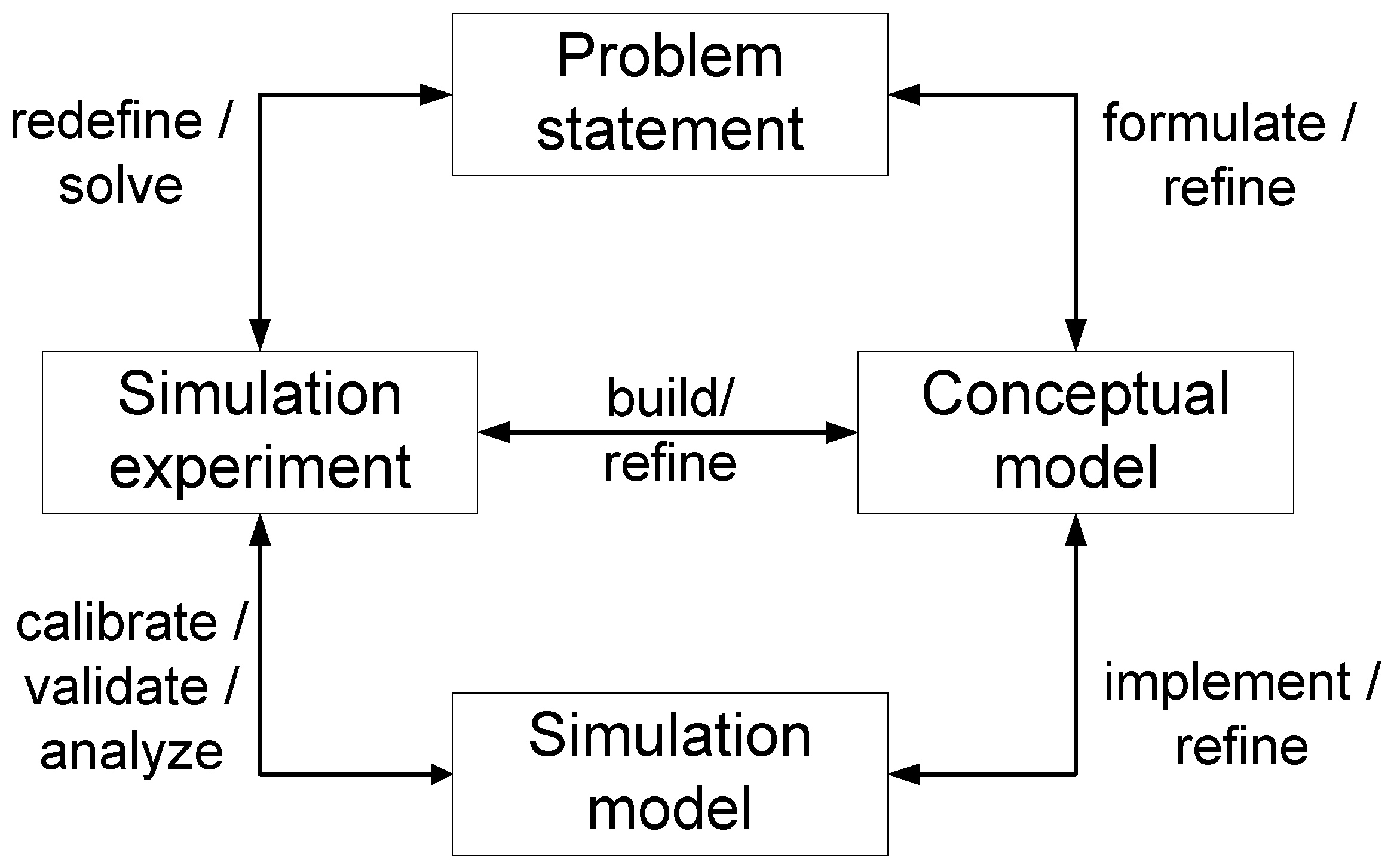

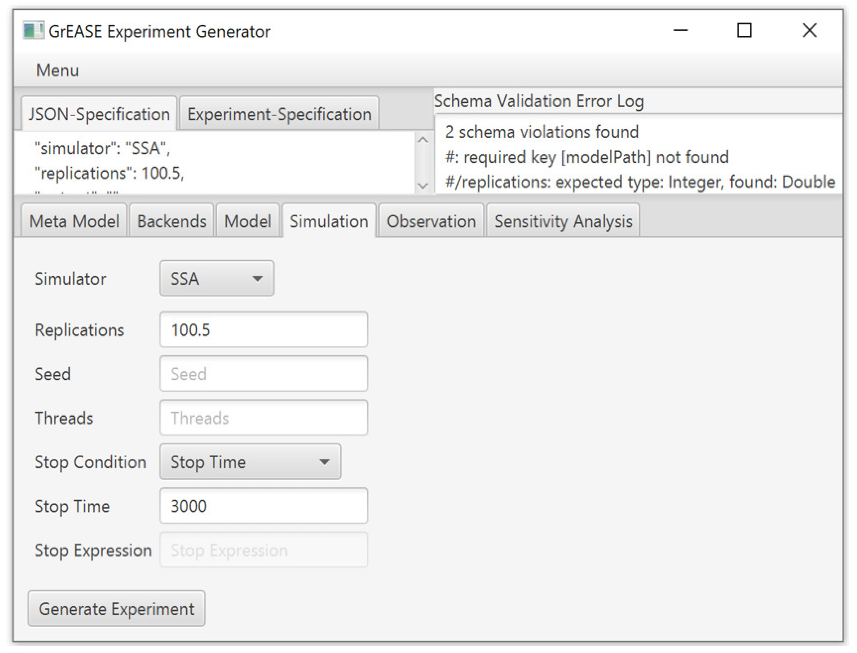


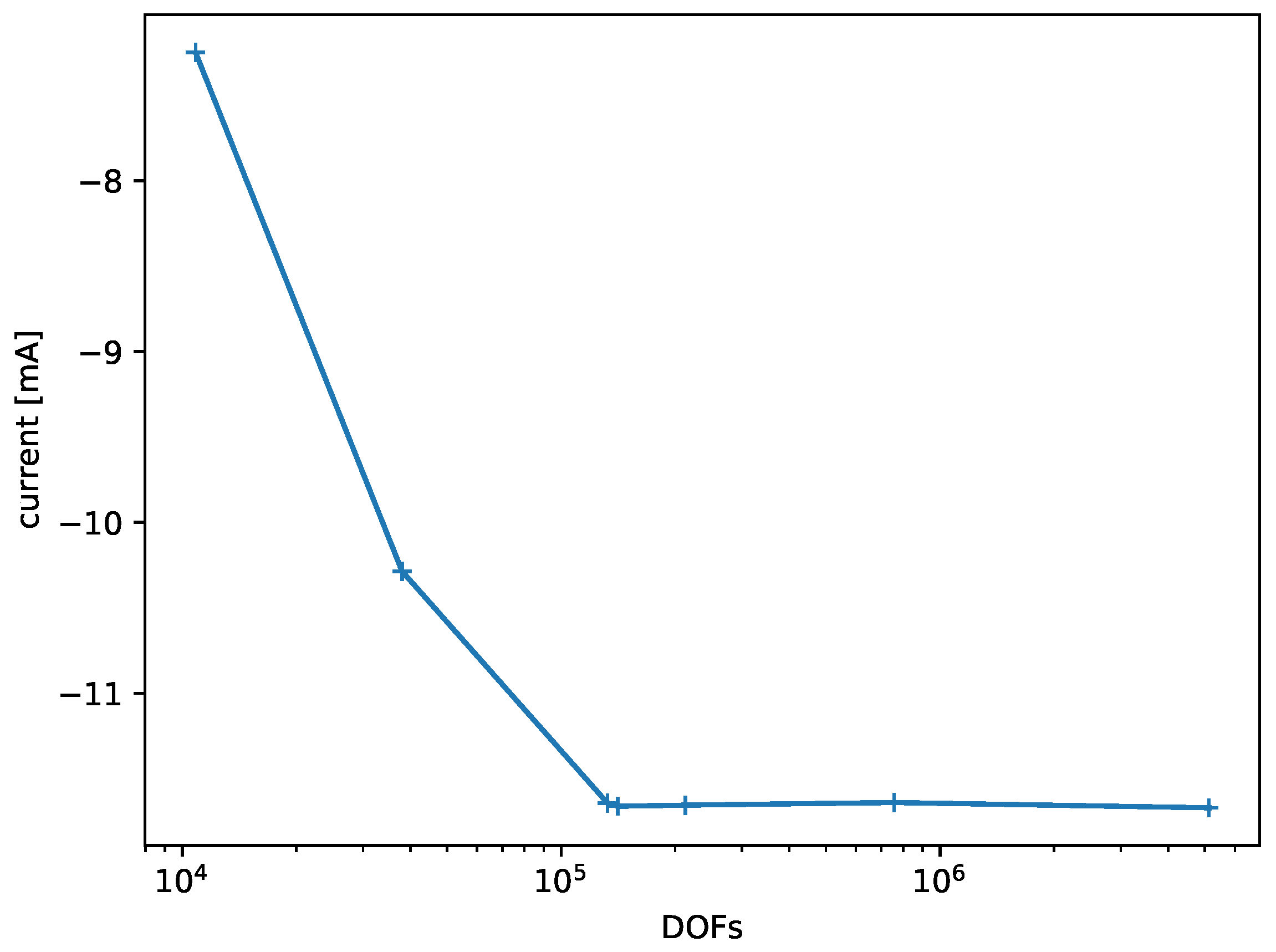

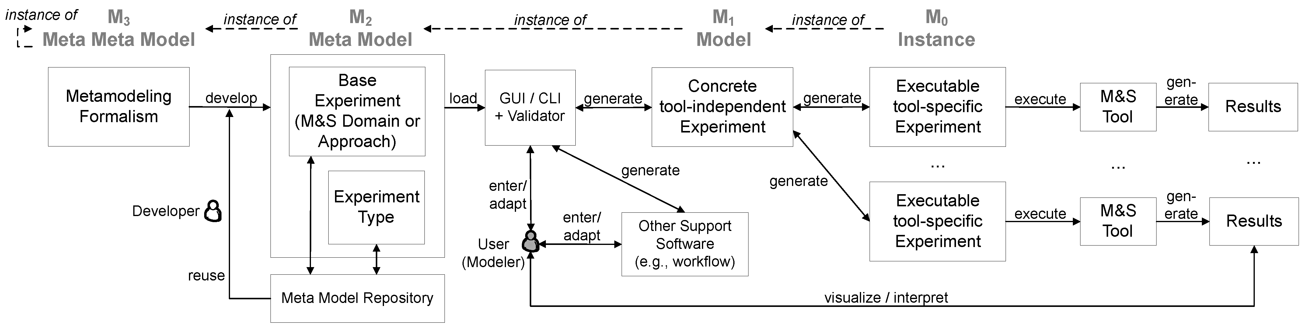
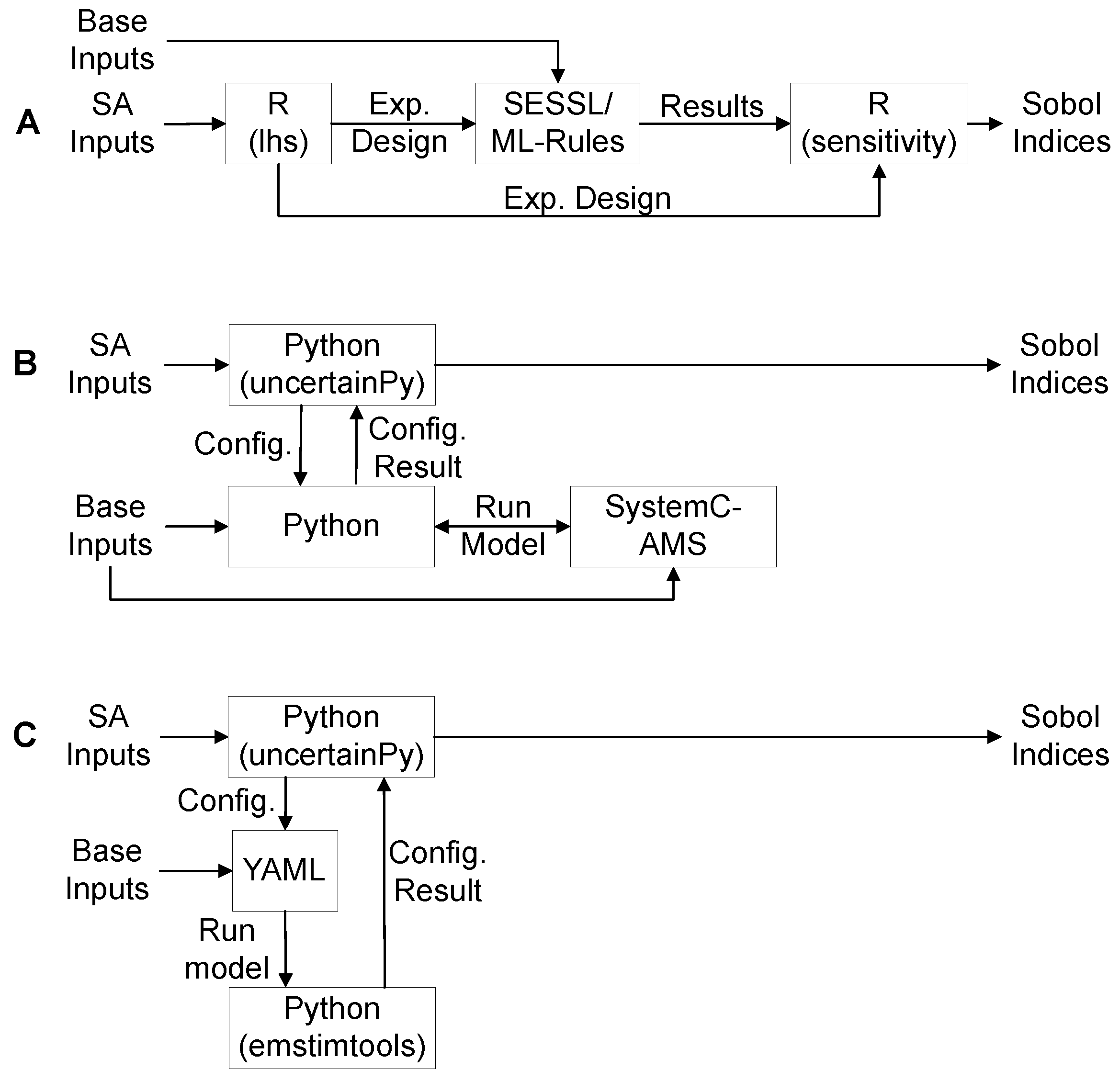
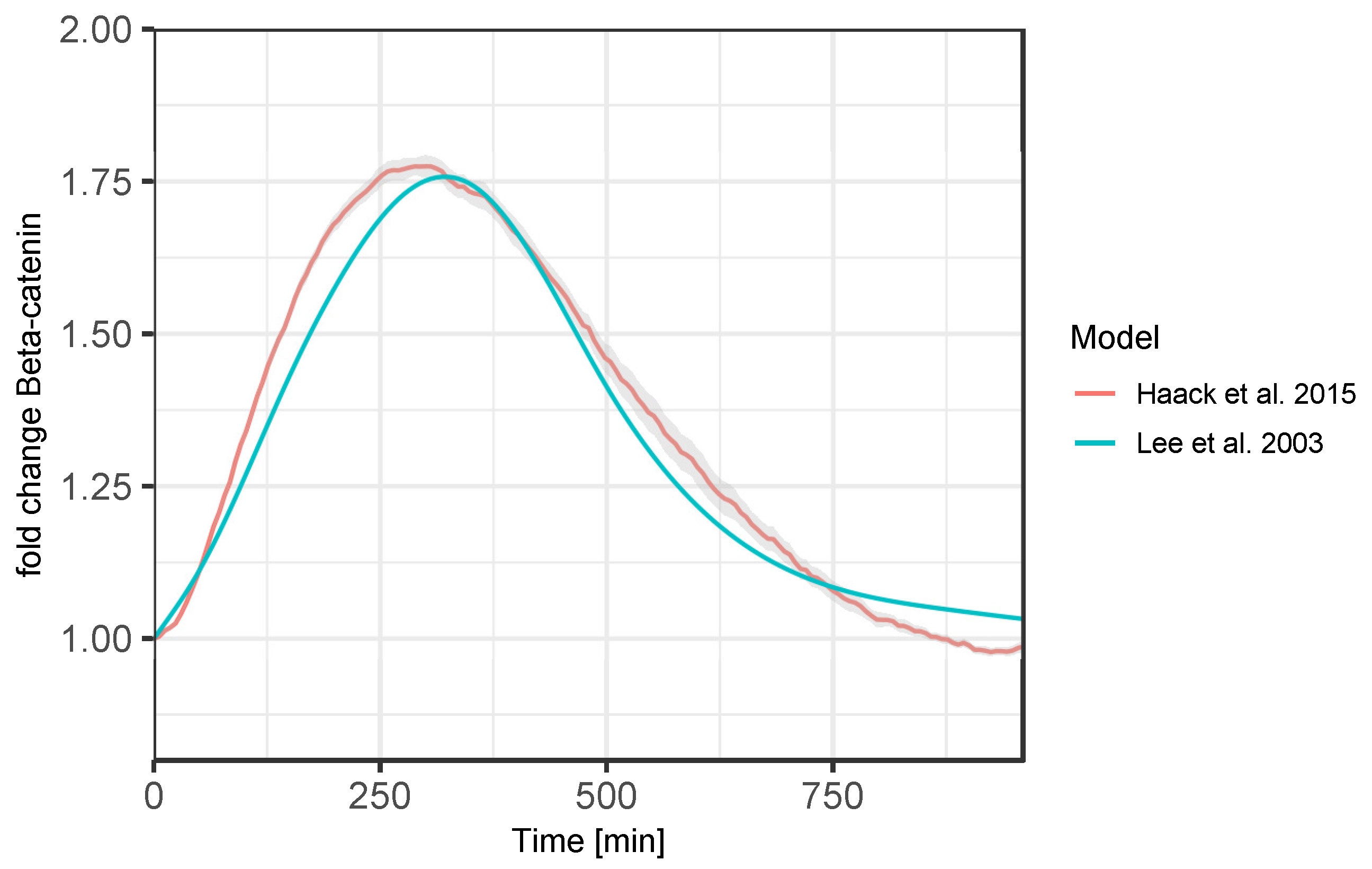
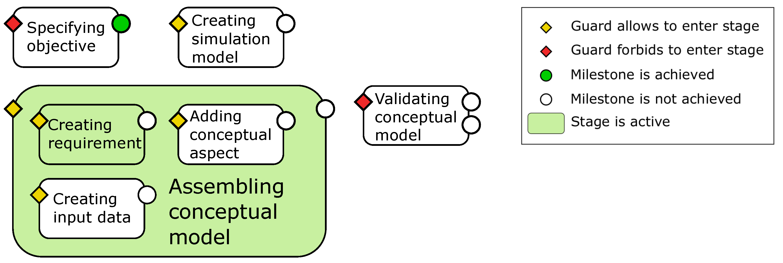