Abstract
Partial least square regression (PLSR) is a reference statistical model in chemometrics. In agronomy, it is used to predict components (response variables y) of chemical composition of vegetal materials from spectral near infrared (NIR) data X collected from spectrometers. PLSR reduces the dimension of the spectral data X by defining vectors that are then used as latent variables (LVs) in a multiple linear model. One difficulty is to determine the relevant dimensionality (number of LVs) for the given data. This step can be very time consuming when many datasets have to be processed and/or the datasets are frequently updated. The paper focuses on an alternative, bypassing the determination of the PLSR dimensionality and allowing for automatizing the predictions. The strategy uses ensemble learning methods, such as averaging or stacking the predictions of a set of PLSR models with different dimensionalities. The paper presents various methods of PLSR averaging and stacking and compares their performances to the usual PLSR on six real datasets on different types of forages. The main finding of the study was the overall superiority of the averaging methods compared to the usual PLSR. We therefore believe that such methods can be recommended to analyze NIR data on forages.
1. Introduction
Near-infrared spectroscopy (NIRS) is a fast and a nondestructive analytical method based on the physical and the chemical properties of organic products. It is used in many agronomic contexts, particularly to evaluate the nutritive quality of forages. Basically, spectral data X (matrix of n observations × p wavelengths) are collected on samples of the material to study (e.g., forages) using a spectrometer, and targeted response variables Y = {y1, …, yk} (k vectors of n observations, e.g., chemical compositions) are measured in a laboratory. For each response variable, a regression model is built between the training data X and y and then used to predict the response variable for new collected spectra. NIRS generate highly correlated variables, then ill-conditioned matrices X. Therefore, for predictions, the usual multiple linear regression model (MLR) is generally not applicable. Partial least squares regression (PLSR) [1,2,3] is a regularization method very efficient for NIRS data in particular in agronomic contexts [4,5,6]. The general principle is to reduce the dimension of X to a limited number a << p of orthogonal n × 1 vectors, referred to as scores, computed to maximize their squared covariance with y. The a scores are finally used as regressor latent variables (LVs) in an MLR.
The determination of the dimensionality a (number of LVs) relevant for the available data is an important step in PLSR modeling. Many strategies have been addressed in the literature for guiding such a determination [7,8,9]. All of these strategies often require decisions based on expertise. In general, some prediction error rates measuring the model performance are estimated for the different dimensionalities a = 0, 1, 2, etc., LVs (for instance by cross-validation; CV) and the dimensionality showing the minimum error rate are selected. For data collected on heterogeneous biological material such as forages, however, it is frequent that the error curve does not have a “U-shape” with a clear minimum, in particular when the sample size of the training dataset becomes large (n > 500 observations). In such a context, the determination of a can become very time consuming in practice, in particular when many datasets (different types of forages and chemical compositions) have to be processed and/or when the datasets are periodically updated with new reference observations (spectra plus laboratory chemical composition). This last case implies many times re-running the overall process of determining relevant dimensionalities a.
An alternative strategy is to automatize the PLSR predictions, bypassing the determination of a. An approach for such automatization, which is presented in this paper, uses ensemble learning methods that average or “stack” the predictions of a set of PLSR models with different dimensionalities a. Some methods of model averaging have already been implemented for PLSR in the past [10,11]. Nevertheless, their performances have not been explored on real datasets of forages. Forage datasets generally contain complex intrinsic material (mixing of stems, leaves, different stages of development, and geographical areas, etc.) and therefore information.
The objective of this paper is to present different averaging and stacking methods, and to compare their performances for a large panel of forage datasets to the usual PLSR (i.e., where an optimal number a of LVs is determined from the examination of an estimate of the prediction error rate). Six spectral datasets X, each collected on a different type of forage, and nine response variables y (each representing a component of the chemical composition) were considered.
The methods of averaging and stacking evaluated in this paper were implemented with the same a priori (i.e., without any preliminary model optimization) for all the datasets {X, y}. This corresponds to an “omnibus” strategy (i.e., a same model and parameterization are applied everywhere), well suited and easy to apply when many datasets of spectra and response variables have to be processed.
2. Theory
2.1. Notations
Vectors and matrices are noted in bold. The paper considers univariate response models. Assume that y is a vector containing n training observations of one given response variable and x a vector of p independent predictors for one given observation. The training observation i is noted (xi, yi) where xi’ (1 × p) is the row i of matrix X (n × p). A new observation to predict is noted (xnew, ynew).
2.2. Prediction Models
2.2.1. Partial Least Squares Regression
Partial least squares regression is a regularization method to solve the ill-conditioned problem
where {X, y} is the training set and
the L2-norm. The general principle is to reduce the dimension of X by computing a limited number a of successive orthogonal n × 1 vectors {t1, t2, …, ta} ≡ T, referred to as “scores”, then used as LVs to regress y by MLR with ordinary least squares. In other words, PLSR replaces in the MLR the high-dimensional and ill-conditioned matrix X by the low-dimensional and orthogonal matrix T.
At each step r (r = 1, …, a), the score vector tr is computed so that it maximizes the squared covariance Cov(tr, y)2. This last constraint is expected to give better prediction performances, for the same given dimensionality a, compared to unconstraint latent regression models, such as principal component regression (PCR). In the particular case of r = 0, the prediction is the mean of y.
Fast and efficient algorithms are available to fit PLSR [12]. By-products of these algorithms allow for re-computing the vector b, referred to as the b-coefficient vector, representing the coefficients of the linear model of Equation (1).
2.2.2. Averaging PLSR
Assume that xnew is a new observation to predict, and that is the prediction returned by the PLSR-averaging model having a number A of LVs (in practice, A will be larger than the dimensionality a selected in the usual PLSR, i.e., corresponding to the minimum prediction error rate). We define the averaging model prediction by:
where wr (r = 0, …, A) is the weight (bounded between 0 and 1) of the model with r LVs, with the constraint:
As indicated in Section 2.2.1, (r = 0 LV) is the simple mean of y. Vector w = {w0, w1, …, wA} represents a pattern of weights. The shape of this pattern is specific to a given averaging method.
Five PLSR-averaging methods (patterns w) are considered in this paper. The first method (AVG) assumes simply a uniform importance for each model, i.e.,
wr = 1/(A + 1).
The three next methods (referred to as AVG-CV, AVG-AIC, and AVG-BIC, respectively) are detailed in Section 2.2.3. All assume that weight wr decreases when the performance of prediction of the model decreases. Assume that dr is a prediction error rate estimated on the training data {X, y} for the PLSR model with r LVs. In the three methods, pattern w is computed from the rates {d0, d1, …, dA} given as input data in a bi-square weighting function [13]. Examples of bi-square function curves are given in Figure 1. The principle is as follows. Let us note the error rate normalized to an upper limit dup that represents the value above which the model with r LVs is removed from the average displayed in Equation (2):
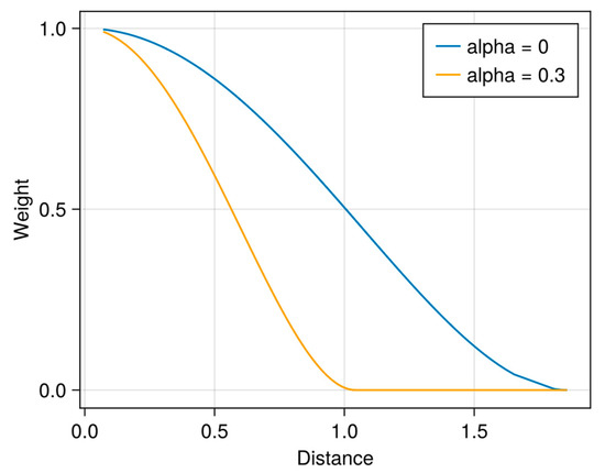
Figure 1.
Example of weight curves computed from a bi-square function for α = 0 and α = 0.3. Distances d were simulated from a Chi-squared distribution (ν = 1 df). In the paper, the “distance” is the error rate of the models.
- = dr/dup if dr < dup
- = 1 if dr ≥ dup (this case implies a null weight).
The bi-square weights are defined by
In practice, PLSR models with dr < dup have a decreasing weight when their error rate dr increases. Models with dr ≥ dup receive a null weight (). To compute the average in Equation (2), the final weights are normalized to sum to 1, i.e.,
The scalar dup is defined by the quantile of order 1 − α (where α is a parameter to set between 0 and 1) of the set d = {d0, d1, …, dA}, i.e., the set of the error rates estimated for the A + 1 PLSR models initially considered in the average. In other words, the 100 × α% less performant models are removed from the average (Equation (2)). Increasing α allows for selecting only the models with the better performances that, in the end, may be expected to return better predictions.
Finally, the fifth method of computing w (AVG-SHENK) was proposed by Shenk et al. [14] for their local (i.e., k-nearest-neighbors based method) PLSR algorithm referred to as “LOCAL”. For each new observation xnew to predict and the PLSR model with r LVs, the weight is defined by the product between the root mean squared x-residuals for x (i.e., the residuals between xnew and its projection to the model PLS space) and the norm of the b-coefficients vector. As before, the final weights are normalized to sum to 1, such as in Equation (3).
2.2.3. Weights for Methods AVG-CV, -AIC, and -BIC
In this paper, three types of error rates d are used to compute w in AVG-CV, -AIC, and -BIC methods.
- AVG-CV: For the PLSR model with r LVs, the error rate dr is the root mean squared error of predictions (RMSEP) estimated on the training data {X, y} from a random K-fold (K = 5) CV (RMSEPCV). The K-fold CV was repeated ten times and dr was computed by the average of the ten RMSEPCV estimates;
- AVG-AIC: dr is the Akaike information criterion [15,16]: AIC = log(SSR) + 2 df, where SSR is the sum of the squared residuals computed on the training data {X, y} and df the complexity (or “effective” dimension or number of degrees of freedom) of the model. The AIC penalty “2 df” increases when the complexity of the model increases (in contrary to SSR) and counter-balances the optimism of SSR to measure the performance of the model for predicting new observations. When several models are compared (i.e., in this paper, the PLSR models with different numbers r of LVs), models with the lowest AICs are considered to be the most performant, as with RMSEPCV in CV. The complexity df is known to be difficult to estimate for PLSR [17,18,19,20]. This is due to the fact that the response variable y is involved in the computation of the LVs, which is not the case, for instance, for PCR models. Nevertheless, approximations are available and, in particular, several methods are detailed and compared in Lesnoff et al. [21]. In the paper, df was computed from the conjugate gradient least square algorithm [22,23]. Since CV and AIC estimate approximately the same type of prediction error [21,24], both methods are expected to estimate close weights patterns w and therefore close results of averaging in Equation (2);
- AVG-BIC: here, dr is another common parsimony criterion, the Bayesian information criterion (BIC) [25]. In BIC, the AIC penalty constant “2” is replaced by log(n), where n is the number of training observations): BIC = log(SSR) + log(n) df. Since the penalty added to SSR is increased compared to AIC, BIC is more conservative and selects (by minimal error rate) models with lower dimensions.
2.2.4. Stacking
Similar to averaging, the stacking method (STACK) consists in a weighted sum of the predictions of the A + 1 PLSR models (r = 0, …, A LVs):
but the coefficients are now estimated from a “top” model ([24]). A K-fold CV is done on the training data {X, y} from which is computed the n × (A + 1) prediction matrix = {, , …, }. The top model consists in regressing y to .
In this paper, the top model is an MLR (without intercept), but other types of models can be used [24]. Contrary to weights wr, the returned MLR coefficients {, , …, } used in Equation (4) are unbounded and can be negative.
3. Materials and Methods
3.1. Datasets and Software
The study datasets are presented in Table 1. The data were collected from forages of tropical areas (TROP1 and TROP2), France (LUS1-2 and THEIX), and Belgium (WAL) and from various species (grasses, legumes, sorghum, mixtures) and various types of vegetal materials (stems, leaves, green, and preserved forages, etc.). All the biological samples collected on the field were dried and grounded, and the absorbance spectra X were collected on Foss NIR Systems Instruments 4500, 5000 or 6500 models. The spectral range 1100 nm to 2498 nm (2 nm step) (Figure 2) was used, except for dataset WAL for which the range was 1300 nm to 2398 nm (2 nm step).

Table 1.
The six study datasets.
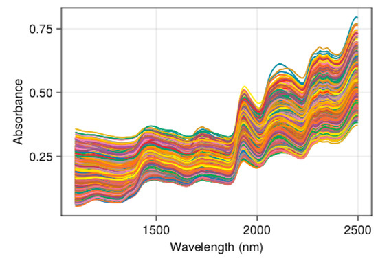
Figure 2.
Example of forage NIR spectra: dataset THEIX (n = 1894).
Nine components of the chemical compositions y (Table 2) were studied. The sampling sizes available for the models ranged from n = 797 observations to n = 5694 observations, depending on the datasets {X, y} (Table 3). Only three datasets (all coming from WAL) contained less than 1000 observations.
Before fitting the models, the spectra were pre-processed by a standard normal variate (SNV) transformation, followed by a Savitzky–Golay 2nd derivation (polynomial of order 2 and window of 11 spectral points). This pre-processing was efficient to predict forage data [21,26], even if not always optimal. Other pre-processing methods could have been used but comparing preprocessing was beyond the objective of this paper. Figure 3 illustrates the variability (clustering) between the six spectral datasets.
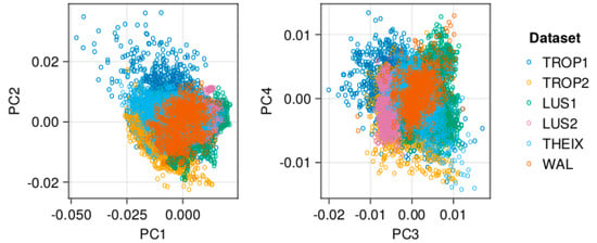
Figure 3.
PCA projection of the spectral data, illustrating that the datasets represent different clusters. The PCA was implemented on the pre-processed data. Percentages of explained variance by the principal components were: PC1 = 40%, PC2 = 20%, PC3 = 11%, and PC4 = 6%.
All the computations (spectra pre-processing and PLSR model computations) were implemented with the package Jchemo [27] written in the free language Julia [28].
Table 2.
Components of the chemical compositions (response variables y) predicted by the models.
Table 2.
Components of the chemical compositions (response variables y) predicted by the models.
| Abbreviation | Unit | Description |
|---|---|---|
| ADF | %DM 1 | Acid detergent fiber [29] |
| ADL | %DM | Acid detergent lignin [29] |
| ASH | %DM | Ashes |
| CF | %DM | Crude fiber [30] |
| CP | %DM | Crude protein [30] |
| DM | % | Dry matter, 103 degrees Celsius, 24 h |
| DMDCELL | %DM | Pepsine–cellulase dry matter digestibility [31] |
| NDF | %DM | Neutral detergent fiber [32] |
| OMDCELL | %OM 2 | Pepsine–cellulase organic matter digestibility [31] |
1 Dry matter; 2 Organic matter.
Table 3.
Number of observations by dataset and response variable (minimum and maximal values of the response variables y are in brackets).
Table 3.
Number of observations by dataset and response variable (minimum and maximal values of the response variables y are in brackets).
| Response | Dataset | |||||
|---|---|---|---|---|---|---|
| Variable (y) | TROP1 | TROP2 | LUS1 | LUS2 | THEIX | WAL |
| ADF | 1530 (8.8, 66.9) | 1126 (12.4, 61.1) | 1310 (10.3, 36.5) | 1355 (17.4, 50.8) | 1507 (15.0, 46.5) | – |
| ADL | 1423 (0.7, 43.1) | 1126 (0.4, 13.6) | – | 1139 (3.0, 10.9) | 1620 (2.7, 27.1) | – |
| ASH | 1597 (1.5, 66.4) | 1476 (0.4, 57.4) | 3526 (4.5, 15.8) | 1242 (5.8, 17.7) | – | – |
| CF | – | 1302 (7.5, 57.3) | – | – | – | 797 (12.0, 42.1) |
| CP | 1564 (1.6, 32.3) | 1389 (0.7, 28.5) | 4029 (3.1, 24.9) | 1612 (2.4, 39.2) | 1564 (3.9, 37.8) | 797 (4.0, 34.2) |
| DM | 1607 (72.2, 97.7) | 1481 (84.7, 98.8) | – | – | – | 797 (89.3, 98.4) |
| DMDCELL | 1459 (9.9, 95.0) | 1137 (14.6, 93.3) | 5194 (41.0, 95.0) | 1584 (38.7, 87.3) | 1386 (20.7, 91.4) | – |
| NDF | 1529 (16.0, 85.7) | 1119 (26.3, 88.0 | 3948 (20.6, 68.4) | 1386 (26.0, 67.8) | 1672 (27.6, 76.9) | – |
| OMDCELL | 1459 (8.6, 94.3) | 1137 (10.9, 90.0) | – | – | – | – |
3.2. Overall Approach to Evaluate the Models
The method of evaluation of the performance of the models was identical for all the datasets.
Let us consider a given dataset {X, y} of sample size n. We randomly split the dataset into two parts:
- A number of ntrain observations {Xtrain, ytrain} are used as a training set to calibrate a given model, say f. This learning step is detailed in Section 3.3;
- A number of ntest observations {Xtest, ytest} (with n = ntrain + ntest) are used to compute the performance of model f learned on {Xtrain, ytrain}. The model performance was defined by the RMSEP computed on the ntest predictions (RMSEPtest).
The split of {X, y} between {Xtrain, ytrain} and {Xtest, ytest} was randomly repeated 100 times to consider, in the results, the sampling variability. The final performance was measured by an average (over the 100 above repetitions) relative error rate. This average relative error rate was defined by the ratio of the mean RMSEPtest (over the 100 replications) to the mean of the response y. This standardization by the mean (as for a coefficient of variation) allowed for summarizing the results of the nine variables together.
Agronomic data, such as forages, have large intrinsic variability due to the heterogeneity of their biological material. If this variability is under-represented in the test set {Xtest, ytest}, this can generate overfitting, optimistic estimates of the performance of the models, and finally misleading conclusions in methods’ comparisons [21]. For preventing such effects, we decided to implement a “severe” split between the training and the test: in each of the 100 above repetitions, the {Xtrain, ytrain} and {Xtest, ytest} represented each half of the dataset (i.e., ntrrain/n = ntest/n = 1/2), while often a softer choice in machine leaning studies is ntrain/n = 2/3 and ntest/n = 1/3.
3.3. Learning Step for Models f
This section describes the learning process of the models f (listed in Table 4) on a given training dataset {Xtrain, ytrain} of sample size ntrain.
3.3.1. Usual PLSR
The usual approach to calibrate a PLSR model is to determine the dimensionality a by taking the minimum value of an estimation of the prediction error. In this paper, a repeated CV (K = 3 blocks; 30 repetitions) was implemented on {Xtrain, ytrain} in which the PLSR dimensionality varied from r = 0 LV and r = 50 LVs. The dimensionality r = a showing the minimum value in the mean RMSEPCV curve (average over the 30 repetitions) was selected. An example of such a curve is given in Figure 4.
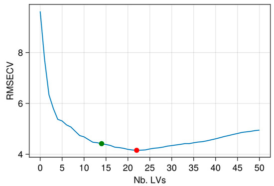
Figure 4.
Example of RMSEPCV curve (mean over 30 repetitions) for PLSR: X-data TROP1 and y-variable ADF. Red point: a = 22 LVs selected by minimum RMSEPCV; Green point: a = 14 LVs selected with Wold’s criterion.
As a remark, considering the all process including the splits “training vs. test” described in the previous section, the approach used here belongs to the family of repeated double CVs [33,34] for PLSR (a CV splits {X, y} to {Xtrain, ytrain} and {Xtest, ytest} to estimate a generalization error and another CV is done internally to {Xtrain, ytrain} for the model calibration, this double process being repeated a number of times).
3.3.2. Parsimonious PLSR (PLSR-P)
For some data, selecting the PLSR dimensionality a by minimal RMSEPCV can generate overparameterization (excessively large values for a). For instance, this can occur when the error rate curve reaches a plateau without increasing values on larger values r or even shows a continuously decreasing trend, instead of a clear “U-shape”, such as that in Figure 4. To get parsimonious PLSR models, a simple heuristic criterion is the “Wold’s ratio” R [35,36,37]. This ratio is defined by
R = 1 − RMSEPCV(r + 1)/RMSEPCV(r)
R represents the relative gain in prediction efficiency after a new LV is added into the model. When selecting a, the iteration r → r + 1 continues until R becomes lower than a threshold value q. In this paper, q was set to 1%. In general, using this ratio returns a dimensionality (a) lower than with the usual selection approach (Figure 4).
3.3.3. PLSR Averaging and Stacking
Contrary to models PLSR and PLSR-P, models AVG, AVG-CV, -AIC, -BIC, and STACK were not preliminarily optimized on training sets. They were directly fitted on {Xtrain, ytrain} after setting an “omnibus” maximal number of LVs (A in Equations (2) and (4)). To keep the operational interest of the methods, A must be given a priori. A heuristic has therefore to be defined (this point is discussed in the final section). Based on our expert experiences on PLSR and our knowledge on the intrinsic heterogeneity of forages data, we defined the following heuristic rule: A = 50 LVs for training sizes ntrain > 400 observations and A = 30 LVs for training sizes ntrain ≤ 400 observations (in this paper, this concerned only WAL datasets). The decrease from 50 LVs to 30 LVs (ntrain ≤ 400) relates to the fact that small datasets cannot support dimensionalities that are too high. Other simple heuristics could be studied (e.g., with functional relations to sample size ntrain) but this goes beyond the objective of this paper.
For AVG-CV, -AIC, and -BIC, two values of parameter α used in the bi-weight function (Section 2.2.2) were considered to study the sensitivity of the methods to this parameter:
- α = 0, i.e., q = max{d0, d1, …, da}, which means that only the less performant model within r = 0, …, 50 LVs is removed from the average;
- α = 0.3, which means that the 30% less performant models within r = 0, …, 50 LVs are removed.
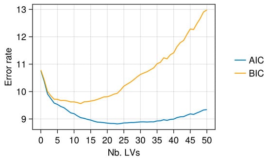
Figure 5.
Example of AIC and BIC curves for PLSR: X-data TROP1 and y-variable ADF.
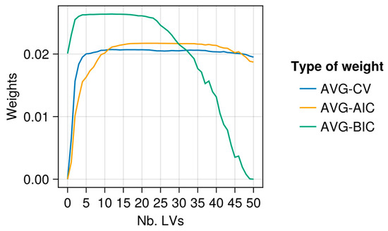
Figure 6.
Example of CV, AIC, and BIC weights for AVG models in which α = 0: X-data TROP1 and y-variable ADF.
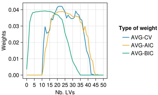
Figure 7.
Same as Figure 6 but with α = 0.3.
Table 4.
PLSR models compared in this study.
Table 4.
PLSR models compared in this study.
| Abbreviation | Method |
|---|---|
| PLSR 1 | Dimensionality is selected by minimal RMSECV. |
| PLSR-P | Parsimonious dimensionality (Wold criterion on RMSECV). |
| “Omnibus” methods | |
| AVG | Averaging with uniform weights. |
| AVG-CV | Averaging with weights computed from CV errors. |
| AVG-AIC | Averaging with weights computed from AIC errors. |
| AVG-BIC | Averaging with weights computed from BIC errors. |
| AVG-SHENK | Averaging with the LOCAL weights [38] |
| STACK | Stacking with MLR as “top” model. |
1 Model taken as reference in this paper.
4. Results
The relative errors estimated for the different models are displayed in Figure 8. Larger standard errors were observed for the WAL datasets, probably due to their lower sample size. Overall, the three less performant models were PLSR-P, PLSR, and AVG-SHENK (except for TROP2 where AVG-SHENK was as performant as other averaging methods).
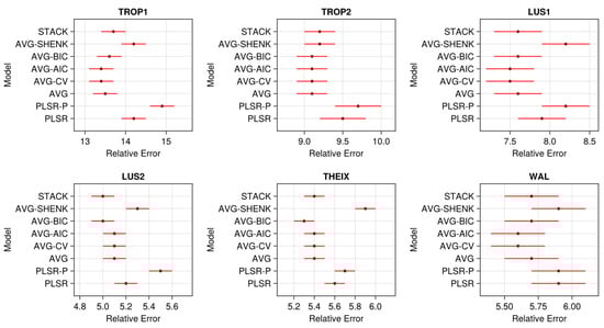
Figure 8.
Relative errors (100 × RMSEPtest/mean(y)) for the study models and datasets. The relative errors were computed over the 100 repetitions of test sets: dots are the means and whiskers are ± the standard errors of the means.
For PLSR, lower dimensionalities a were selected for WAL datasets (a ≤ 20) compared to the others, in relation to their lower size. As expected, PLSR-P also selected lower dimensionalities a than the usual PLSR (Table 5). Nevertheless, PLSR-P was always less efficient (Figure 8) than PLSR. This indicates that selecting high values a in PLSR (up to a = 50 LVs in certain repetitions; Table 5) did not generate overfitting on these data.
Table 5.
Dimensionality a (nb. LVs) selected by RMSEPCV for PLSR and PLSR-P models.
Globally, averaging models showed better performances than stacking (Figure 8), even if both types of methods returned close relative errors. On our forage data, building a top model over the (A + 1) PLSR models was therefore not advantageous when compared to a direct averaging of the predictions.
Within the averaging methods, computing model weights from CV-, AIC-, or BIC-error rates has tended to slightly increase the performances compared to a uniform average. Nevertheless, the differences were very low (e.g., for LUS2 in Figure 8, the relative error was 5.0% for AVG-BIC vs. 5.1% for AVG) with orders of magnitude that have no agronomic importance in practice. Differences between the weighting methods were also clearly dataset dependent (e.g., in TROP2, AVG was almost equal to other averaging). Even with a uniform weighting, it is important to note that averaging was always better than the usual PLSR.
For CV-, AIC-, and BIC-averaging, the effect of parameter α (Figure 9) was dataset and method dependent, without showing a clear pattern. For instance, removing the 30% less performant models in Equation (2) (i.e., α = 0.3) did not improve the predictions for BIC weighting (all the datasets), while this was more successful in other situations (e.g., for CV-weighting).
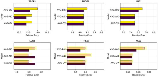
Figure 9.
Mean relative errors (100 × RMSEPtest/mean(y)) for the study models, datasets, and values of parameter α: α = 0 in purple, α = 0.3 in yellow.
5. Discussion and Conclusions
The major finding of this paper is the overall superiority of the averaging methods compared to the usual PLSR selecting dimensionality a by minimum RMSEPCV. In our evaluation, we chose a severe splitting of the data (test set = half of the data) to prevent optimistic estimates of performances, which can occur frequently when the study materials have complex structures. To check the consistency of the results, we replicated all the same computations presented in this paper but with the more usual splitting {training set = 2/3, test set = 1/3}. The same types of patterns were observed in the performances (not detailed in this text), in particular the superiority of the averaging methods to the usual PLSR.
When using averaging or stacking, the maximal dimensionality A has to be set as input parameter. In practice, A can be optimized based on each dataset {X, y}, as the dimensionality a in the usual PLSR. However, the methods have the advantage of allowing a strategy where A is set a priori as an omnibus value, with the expectation that this value will provide results that are sufficiently efficient even if not fully optimal for each dataset. Such a strategy was implemented in this work. The a priori choices A = 50 LVs (ntrain > 400) and A = 30 LVs (ntrain ≤ 400) appeared relevant for our forages data. More generally, for any type of data, relevant orders of magnitude of A can be easily estimated on a few preliminary validation samples. For instance, with a few runs of CV on other datasets than those presented in this paper (containing lower heterogeneity and lower sample sizes; ntrain ≤ 200), we observed that A = 20 LVs was very efficient for these data. This easy and fast calibration process can help the user to find a value of A that will be efficient “everywhere” on his data.
On our data, the SHENK weights [38] did not provide good performances. This was not in adequation with the observations of Zhang et al. [11] on smaller and less complex datasets. Stacking results were also disappointing. Optimizing the weights by a top regression model did not improve the prediction performances.
Averaging with CV-, AIC-, and BIC-weighting appeared to be the best methods overall. Nevertheless, uniform weighting was often almost as performant. The AVG method has the advantage of being simpler and much faster to compute (no need to internally estimate training error rates on {Xtrain, ytrain}, required to compute the variable model weights). AVG can therefore be recommended for a fast strategy, providing efficient results even if not always optimal.
This paper focused on forages, a priority material studied in feed research teams for which significant data in numbers and representativity are available. Forage data have the characteristic to contain a high level of heterogeneity due to scattering effects in the NIR signals, diversity of origins, species, climate, conditions of data collections, spectrometers, etc. The presented averaging methods may be advantageous for other materials, such as foods and other agricultural products, when they present heterogeneity. The readers are encouraged to test these generic and easy-to-implement methods on many other types of materials than forages to eventually validate this guess.
Finally, averaging methods presented in this paper can be easily embedded in pipelines of local PLSR [26,39,40,41,42]. Such pipelines fit a PLSR model for each new observation to predict, after having selected a neighborhood of this observation. Local PLSR are particularly efficient when the relation between y and X is nonlinear. This occurs for instance when the data contain clustering and the relation y = f(X) varies between clusters. As for PLSR, local PLSR can become time consuming to optimize when many datasets {X, y} have to be processed. Again, with the objective of automatized predictions, local AVG PLSR methods can represent fast and safe alternatives to methods requiring time consuming calibrations.
Author Contributions
Conceptualization and methodology, M.L. and J.-M.R.; software, M.L.; data curation, D.A., P.B., C.B., L.B., F.P., J.A.F.P. and P.V.; writing—original draft preparation, M.L.; writing—review and editing, M.L., D.A., P.B., C.B., L.B., F.P., J.A.F.P., P.V. and J.-M.R. All authors have read and agreed to the published version of the manuscript.
Funding
This research received no external funding.
Data Availability Statement
The datasets presented in this paper are private and not freely available.
Acknowledgments
We thank Cirad, CRA-W, and Inrae for giving us access to the datasets. We are also grateful to the three anonymous reviewers for their constructive remarks that improved this paper.
Conflicts of Interest
The authors declare no conflict of interest.
References
- Höskuldsson, A. PLS Regression Methods. J. Chemom. 1988, 2, 211–228. [Google Scholar] [CrossRef]
- Wold, H. Nonlinear Iterative Partial Least Squares (NIPALS) Modeling: Some Current Developments. In Multivariate Analysis II; Krishnaiah, P.R., Ed.; Academic Press: Cambridge, MA, USA, 1973; pp. 383–407. [Google Scholar]
- Wold, S.; Sjöström, M.; Eriksson, L. PLS-Regression: A Basic Tool of Chemometrics. Chemom. Intell. Lab. Syst. 2001, 58, 109–130. [Google Scholar] [CrossRef]
- Dardenne, P.; Sinnaeve, G.; Baeten, V. Multivariate Calibration and Chemometrics for near Infrared Spectroscopy: Which Method? J. Near Infrared Spectrosc. JNIRS 2000, 8, 229–237. [Google Scholar] [CrossRef]
- Wang, F.; Zhao, C.; Yang, H.; Jiang, H.; Li, L.; Yang, G. Non-Destructive and in-Site Estimation of Apple Quality and Maturity by Hyperspectral Imaging. Comput. Electron. Agric. 2022, 195, 106843. [Google Scholar] [CrossRef]
- Chu, X.; Li, R.; Wei, H.; Liu, H.; Mu, Y.; Jiang, H.; Ma, Z. Determination of Total Flavonoid and Polysaccharide Content in Anoectochilus Formosanus in Response to Different Light Qualities Using Hyperspectral Imaging. Infrared Phys. Technol. 2022, 122, 104098. [Google Scholar] [CrossRef]
- Gowen, A.A.; Downey, G.; Esquerre, C.; O’Donnell, C.P. Preventing Over-Fitting in PLS Calibration Models of near-Infrared (NIR) Spectroscopy Data Using Regression Coefficients. J. Chemom. 2011, 25, 375–381. [Google Scholar] [CrossRef]
- Kalivas, J.H. Multivariate Calibration, an Overview. Anal. Lett. 2005, 38, 2259–2279. [Google Scholar] [CrossRef]
- Westad, F.; Marini, F. Validation of Chemometric Models—A Tutorial. Anal. Chim. Acta 2015, 893, 14–24. [Google Scholar] [CrossRef]
- Silalahi, D.D.; Midi, H.; Arasan, J.; Mustafa, M.S.; Caliman, J.-P. Automated Fitting Process Using Robust Reliable Weighted Average on Near Infrared Spectral Data Analysis. Symmetry 2020, 12, 2099. [Google Scholar] [CrossRef]
- Zhang, M.H.; Xu, Q.S.; Massart, D.L. Averaged and Weighted Average Partial Least Squares. Anal. Chim. Acta 2004, 504, 279–289. [Google Scholar] [CrossRef]
- Andersson, M. A Comparison of Nine PLS1 Algorithms. J. Chemom. 2009, 23, 518–529. [Google Scholar] [CrossRef]
- Cleveland, W.S.; Grosse, E. Computational Methods for Local Regression. Stat. Comput. 1991, 1, 47–62. [Google Scholar] [CrossRef]
- Shenk, J.S.; Westerhaus, M.O. Population Definition, Sample Selection, and Calibration Procedures for Near Infrared Reflectance Spectroscopy. Crop Sci. 1991, 31, 469. [Google Scholar] [CrossRef]
- Hurvich, C.M.; Tsai, C.-L. Bias of the Corrected AIC Criterion for Underfitted Regression and Time Series Models. Biometrika 1991, 78, 499–509. [Google Scholar] [CrossRef]
- Hurvich, C.M.; Tsai, C.-L. Regression and Time Series Model Selection in Small Samples. Biometrika 1989, 76, 297–307. [Google Scholar] [CrossRef]
- Ildiko, F.E.; Friedman, J.H. A Statistical View of Some Chemometrics Regression Tools. Technometrics 1993, 35, 109–135. [Google Scholar] [CrossRef]
- Krämer, N.; Sugiyama, M. The Degrees of Freedom of Partial Least Squares Regression. J. Am. Stat. Assoc. 2011, 106, 697–705. [Google Scholar] [CrossRef] [Green Version]
- Seipel, H.A.; Kalivas, J.H. Effective Rank for Multivariate Calibration Methods. J. Chemom. 2004, 18, 306–311. [Google Scholar] [CrossRef]
- van der Voet, H. Pseudo-Degrees of Freedom for Complex Predictive Models: The Example of Partial Least Squares. J. Chemom. 1999, 13, 195–208. [Google Scholar] [CrossRef]
- Lesnoff, M.; Roger, J.-M.; Rutledge, D.N. Monte Carlo Methods for Estimating Mallows’s Cp and AIC Criteria for PLSR Models. Illustration on Agronomic Spectroscopic NIR Data. J. Chemom. 2021, 35, e3369. [Google Scholar] [CrossRef]
- Björck, Å. Numerical Methods for Least Squares Problems; Society for Industrial and Applied Mathematics: Philadelphia, PA, USA, 1996; ISBN 978-0-89871-360-2. [Google Scholar]
- Hansen, P.C. Rank-Deficient and Discrete Ill-Posed Problems; Society for Industrial and Applied Mathematics: Philadelphia, PA, USA, 1998; ISBN 978-0-89871-403-6. [Google Scholar]
- Hastie, T.; Tibshirani, R.; Friedman, J. The Elements of Statistical Learning: Data Mining, Inference, and Prediction, 2nd ed.; Springer: New York, NY, USA, 2009. [Google Scholar]
- Schwarz, G. Estimating the Dimension of a Model. Ann. Statist. 1978, 6, 461–464. [Google Scholar] [CrossRef]
- Lesnoff, M.; Metz, M.; Roger, J.-M. Comparison of Locally Weighted PLS Strategies for Regression and Discrimination on Agronomic NIR Data. J. Chemom. 2020, 10, e3209. [Google Scholar] [CrossRef]
- Lesnoff, M. Jchemo: A Julia Package for Dimension Reduction, Regression and Discrimination for Chemometrics; CIRAD, UMR SELMET: Montpellier, France, 2021. [Google Scholar]
- Bezanson, J.; Edelman, A.; Karpinski, S.; Shah, V.B. Julia: A Fresh Approach to Numerical Computing. SIAM Rev. 2017, 59, 65–98. [Google Scholar] [CrossRef] [Green Version]
- Van Soest, P.J.; Robertson, J.B. Systems of Analysis for Evaluating Fibrous Feeds. In IDRC No 134; IDRC: Ottawa, ON, Canada, 1980; pp. 49–60. [Google Scholar]
- AOAC. Official Methods of Analysis of the Association of Official Analytical Chemists; AOAC International Publishing: Gaithersburg, MD, USA, 2005. [Google Scholar]
- Aufrère, J.; Michalet-Doreau, B. In Vivo Digestibility and Prediction of Digestibility of Some By-Products. In Feeding Value of by-Products and Their Use by Beef Cattle; Boucqué, C.V., Fiems, L.O., Cottyn, B.G., Eds.; Commission of the European Communities Publishing: Brussels, Belgium; Luxembourg, 1983; pp. 25–33. [Google Scholar]
- Van Soest, P.J.; Robertson, J.B.; Lewis, B.A. Methods for Dietary Fiber, Neutral Detergent Fiber, and Nonstarch Polysaccharides in Relation to Animal Nutrition. J. Dairy Sci. 1991, 74, 3583–3597. [Google Scholar] [CrossRef]
- Filzmoser, P.; Liebmann, B.; Varmuza, K. Repeated Double Cross Validation. J. Chemom. 2009, 23, 160–171. [Google Scholar] [CrossRef]
- Krstajic, D.; Buturovic, L.J.; Leahy, D.E.; Thomas, S. Cross-Validation Pitfalls When Selecting and Assessing Regression and Classification Models. J. Cheminform. 2014, 6, 10. [Google Scholar] [CrossRef] [PubMed] [Green Version]
- Andries, J.P.M.; Vander Heyden, Y.; Buydens, L.M.C. Improved Variable Reduction in Partial Least Squares Modelling Based on Predictive-Property-Ranked Variables and Adaptation of Partial Least Squares Complexity. Anal. Chim. Acta 2011, 705, 292–305. [Google Scholar] [CrossRef] [PubMed]
- Schaal, S.; Atkeson, C.G.; Vijayakumar, S. Scalable Techniques from Nonparametric Statistics for Real Time Robot Learning. Appl. Intell. 2002, 17, 49–60. [Google Scholar] [CrossRef]
- Wold, S. Cross-Validatory Estimation of the Number of Components in Factor and Principal Components Models. Technometrics 1978, 20, 397–405. [Google Scholar] [CrossRef]
- Shenk, J.; Westerhaus, M.; Berzaghi, P. Investigation of a LOCAL Calibration Procedure for near Infrared Instruments. J. Near Infrared Spectrosc. 1997, 5, 223. [Google Scholar] [CrossRef]
- Kim, S.; Okajima, R.; Kano, M.; Hasebe, S. Development of Soft-Sensor Using Locally Weighted PLS with Adaptive Similarity Measure. Chemom. Intell. Lab. Syst. 2013, 124, 43–49. [Google Scholar] [CrossRef] [Green Version]
- Shen, G.; Lesnoff, M.; Baeten, V.; Dardenne, P.; Davrieux, F.; Ceballos, H.; Belalcazar, J.; Dufour, D.; Yang, Z.; Han, L.; et al. Local Partial Least Squares Based on Global PLS Scores. J. Chemom. 2019, 33, e3117. [Google Scholar] [CrossRef]
- Allegrini, F.; Fernández Pierna, J.A.; Fragoso, W.D.; Olivieri, A.C.; Baeten, V.; Dardenne, P. Regression Models Based on New Local Strategies for near Infrared Spectroscopic Data. Anal. Chim. Acta 2016, 933, 50–58. [Google Scholar] [CrossRef]
- Minet, O.; Baeten, V.; Lecler, B.; Dardenne, P.; Fernández Pierna, J.A. Local vs. Global Methods Applied to Large near Infrared Databases Covering High Variability. In Proceedings of the 18th International Conference on Near Infrared Spectroscopy; IM Publications Open LLP: Copenhagen, Denmark, 2019; pp. 45–49. ISBN 978-1-906715-27-4. [Google Scholar]
Publisher’s Note: MDPI stays neutral with regard to jurisdictional claims in published maps and institutional affiliations. |
© 2022 by the authors. Licensee MDPI, Basel, Switzerland. This article is an open access article distributed under the terms and conditions of the Creative Commons Attribution (CC BY) license (https://creativecommons.org/licenses/by/4.0/).