1. Introduction
In recent decades, new levels of complexity and miniaturisation have been reached in micro- and nanotechnology manufacturing [
1]. As described in various road maps such as the ITRS or IRDS, structure sizes continue to decrease, while wafer sizes increase in order to achieve the highest possible throughput [
2,
3]. Highly accurate metrology is needed to achieve reproducible and error-free fabrication as well as the imaging of structures in various fields, such as nanoelectronics and semiconductors [
4].
In the fabrication as well as the characterisation of nanostructures, many different alternative tools, in contrast to conventional methods, have been established, such as optical systems, tip-based systems as well as imprint tools [
5]. However, most of these established technologies are limited to their measurement range. Especially with tip-based methods such as atomic force microscopy [
6], there are usually a few square micrometres of area available in which the surface can be scanned with high precision.
In order to meet these challenges of high-precision positioning and, at the same time, the possibility of positioning on large areas in the millimetre range, nanopositioning and nanomeasuring machines can fill this gap. In the past decades, numerous research groups have worked on the development and improvement of nanopositioning technology [
7].
For more than 20 years now, the Institute for Process Measurement and Sensor Technology at the Technische Universität Ilmenau has invested a great deal of work in the development of nanopositioning technology. The first three-dimensional positioning machine was developed with a movement range of 25 mm × 25 mm × 5 mm [
8]. Subsequently, another machine was developed with a much larger measuring and movement range: 200 mm × 200 mm × 25 mm [
9]. With these machines, the focus was primarily on a large movement range in all three spatial axes (
x,
y and
z direction).
These machines can be equipped with various tools. For example, they can be used for characterisation by means of an autofocus sensor or an atomic force microscope (AFM) and for the production of structures via direct laser writing (DLW), nanoimprint lithography (NIL) and tip-based via field emission scanning probe lithography (FESPL) [
5].
Especially for wafer-based technologies, it is of particular importance to have a stable z axis, which is why, in the development of a new type of nanopositioning machine, it was decided to limit the range of motion to two dimensions.
This planar machine in combination with a tip-based measuring system was designed and developed by SIOS GmbH in cooperation with the companies IMMS GmbH and nano analytik GmbH in Ilmenau [
10].
With its range of motion of Ø100 mm, this newly developed nanopositioning machine is used to explore atomic force microscopy on large surfaces with ultimate precision.
In previous contributions, the enormous potential of the combination of a tip-based measurement system and the nanopositioning technique could yield first results. Line scans over millimetre ranges [
11] as well as area scans [
10] could be demonstrated, where the tip-based system realises the movement in the
z direction and the machine table moves the sample in the
x and
y direction.
In this paper, the focus lies on the positioning accuracy of the machine table itself, how the deviation from the given trajectory increases with higher speed. First of all, after the presentation and classification of various positioning systems, the machine which is used and its structure are explained in more detail. Subsequently, the components available are described and the basic control scheme is explained. The analysis of the positioning accuracy starts with the investigation of the static state in closed-loop control. The deviation from the predefined trajectory is to be considered in different traversing scenarios, such as linear and circular movements up to the maximum velocity of 20 mm/s. Additionally, the tip-based system can provide information about the z noise. This is shown by AFM scans on SiC steps with hundreds of picometre height by comparing the scans with the machine table switched on and off. The main focus of this contribution is the metrological investigation of the planar nanopositioning machine.
2. State of the Art—Nanopositioning and Nanomeasuring Machines
In general, different approaches are used in nanopositioning and nanomeasuring technology. These include the sample-scanning mode, mixed-scanning mode and scanning probe mode [
12]. In the sample-scanning mode, the measuring tool remains in a fixed position while the sample is moved by a machine table. In the scanning probe mode, the measuring tool is moved in all three spatial directions while the sample to be investigated is fixed.
In 1890, Ernst Abbe described an important principle of length measuring technology, where the measuring apparatus is to be arranged in such a way that the distance to be measured forms the straight-line continuation of the graduation, serving as a scale [
13,
14]. In this measuring arrangement, length measuring deviations, which are caused by systematic or accidental tilting, are reduced [
14].
This Abbe comparator principle [
13] was further developed into the extended three-dimensional Abbe comparator [
15,
16]. The nanopositioning machines developed at the Technische Universität Ilmenau are based on this principle, as this concept offers the possibility of using the high accuracy of the laser interferometer for 3D measurements. Because in the sample-scanning mode the probe as well as the measuring system are attached to a metrological frame, the Abbe comparator principle is fulfilled in all three measuring axes in which the length- and angle measuring systems do not have to be displaced. Based on this concept, the nanopositioning and measuring machine NMM-1 was developed, where three interferometric length measuring systems intersect in the touching point of the probe [
17]. This way, the Abbe comparator concept is complied in all three directions of motion. In order to avoid higher-order error influences due to angular tilt, additional angular sensors are mounted. These sensors are detecting the angular tilt, which is compensated for by the drive system.
Due to the overall concept of the machine, a resolution of 0.1 nm and a measurement uncertainty of 9 nm can be achieved in the measuring range of 25 mm × 25 mm × 5 mm [
8].
After evaluating and testing the NMM-1, experience was gained and a new nanopositioning and measuring machine—the so-called NPMM-200—was developed, which is also based on the sample-scan mode and allows a significantly larger measuring range of 200 mm × 200 mm × 25 mm as well as an increase in performance in terms of position resolution [
18]. Here, a three-dimensional measurement uncertainty of 30 nm was achieved [
4].
The company
IBS Precision developed a machine with a significantly larger measuring range: the nanocoordinate measuring machine ISARA 400 with a positioning range of 400 mm × 400 mm × 100 mm. However, the mixed-scanning mode is used here, where the machine table and the measuring tool are moved. The Abbe principle is also fulfilled here, due to the arrangement of the interferometric length measuring systems. The ISARA 400 achieves a measuring resolution of 1.6 nm and a measuring uncertainty of 100 nm [
19].
The positioning machines presented have been specially developed to be able to move in all three measuring axes. Particular attention was placed on enabling a high movement range in the z direction. For very sensitive measuring tools such as tip-based systems, however, it is essential to have a particularly stable z axis during the movement of the sample stage.
For this reason, the nanofabrication machine (NFM-100) was developed to demonstrate and investigate the combination of tip-based technology and nanopositioning technology. This machine only moves in the x and y direction within a movement range of 100 mm in diameter. In principle, it follows the same principle, i.e., the sample-scanning mode, as the NMM-1 and the NPMM-200 but without allowing movement in the z direction.
3. Setup of the Planar Nanopositioning Machine
The newly developed planar nanofabrication machine has been specially designed for measurement and fabrication processes on wafer sizes of 4 inches.
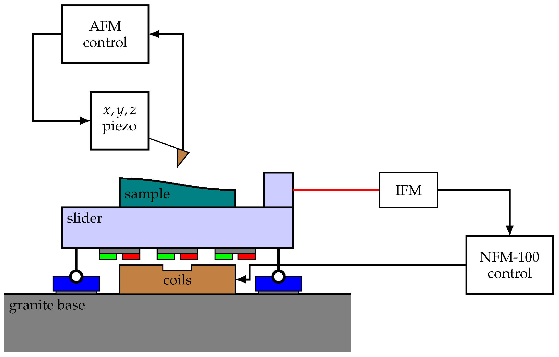
Figure 1 shows a side view of the machine setup itself. As mentioned, a tip-based measuring system is installed as a measuring tool. This AFM system uses active microcantilevers and has a three-dimensional motion range of 10 µm × 10 µm × 5 µm due to the piezo scanning unit. These self-actuated and self-sensing microcantilevers are induced to oscillate by a thermomechanical actuator. This actuator consists of different layers with different coefficients of thermal expansion. The deflection readout of the cantilever is realised by a Wheatstone bridge. Scanning speeds of up to 50 µm/s have already been demonstrated with this tip-based system [
20].
The whole setup is operated in a climate-controlled and vibration-isolated environment. The slider is guided aerostatically on three air bearings from NewWay [
21]. The position is measured by differential interferometers (IFM) [
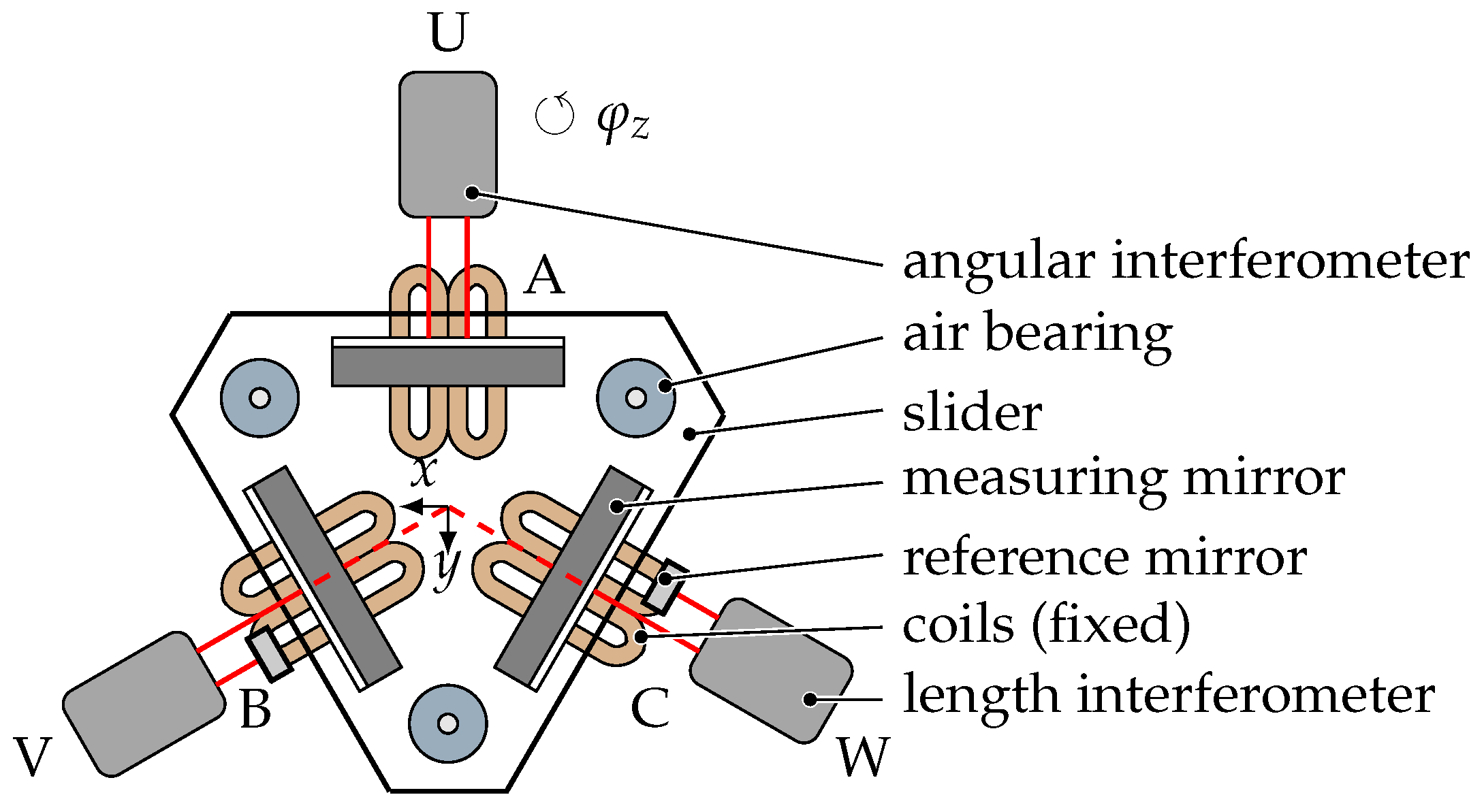
22]. The length measuring systems as well as the actuators are arranged in a single plane and at an angle of 120 degrees between each other, as can be seen in
Figure 2.
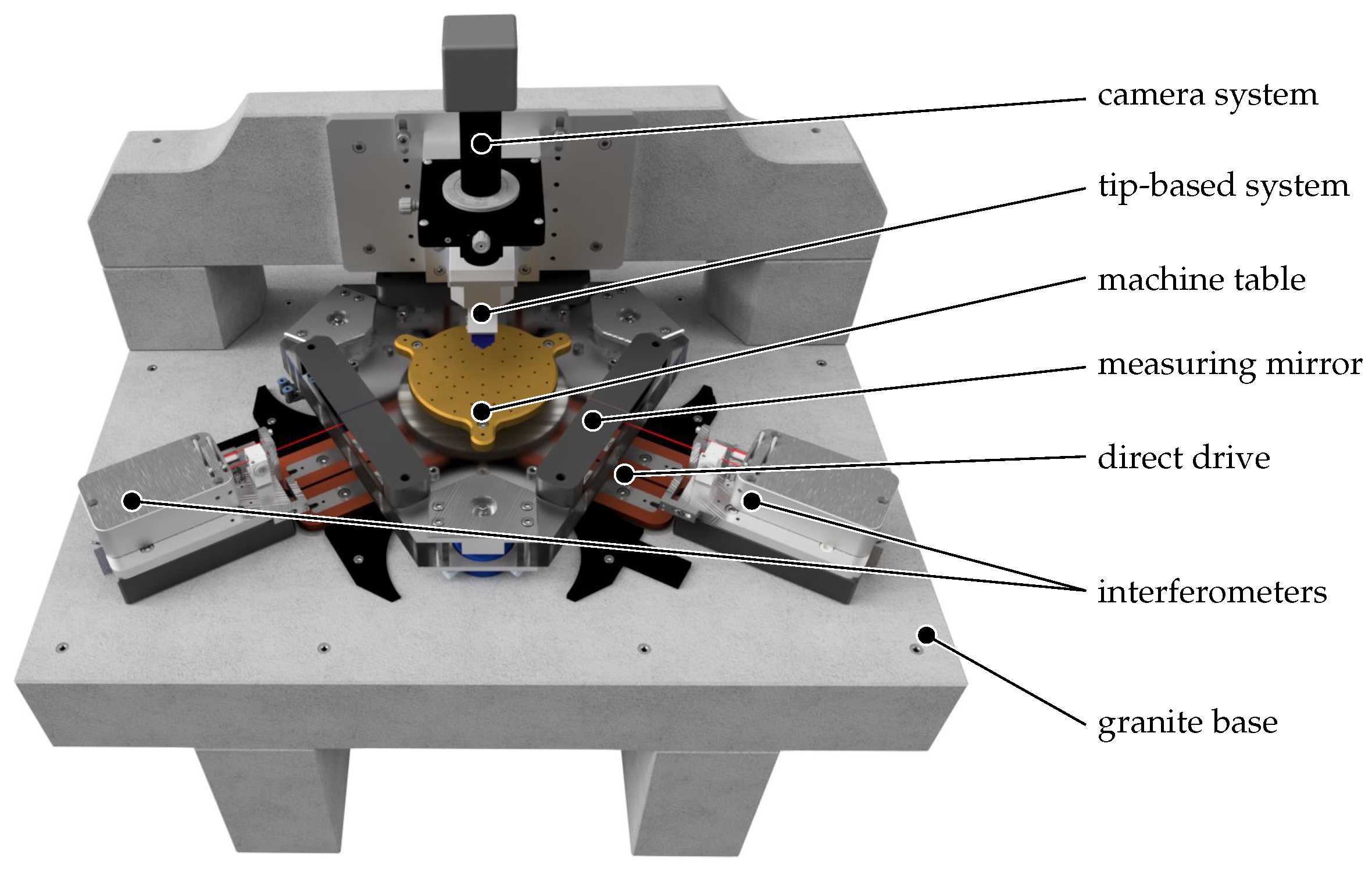
Aerostatic guide elements were chosen for the demanding nanometre-precise positioning because they provide a number of advantages, such as extremely low friction and low vibration during the movement [
21]. These elements are mounted to the machine slider and hover on the planar granite base of the NFM-100 (see
Figure 3), supplied with pressurised air by flexible tubing. Because there is no mechanical contact with this type of guidance, stick–slip effects can be eliminated. In addition, these air bearings are characterised by high repeatability [
23].
For positioning of the slider, the NFM-100 uses a planar direct drive system. Three actuators based on electromagnetic force generation are used here, which enable a contactless force transfer. Each actuator consists of two fixed coils that act on magnets attached to the slider, i.e., the machine table. The drive forces of the three linear actuators act simultaneously on the slider. The 120
arrangement allows a resulting force in any direction within the
x-
y plane and additionally a rotation around the
z axis can be generated [
24]. Accordingly, this results in a circular range of motion.
Three differential plane-mirror interferometers, which offer especially high thermal stability due to their symmetric optical design, are used as length measurement systems [
22]. The laser source for these differential interferometers is a stabilised He-Ne laser, which provides a relative frequency stability of 2 × 10
. The evaluation electronic uses an arctan demodulation technique with a path resolution of 5 pm [
25].
By setting up the interferometers with an external reference beam, the measurement systems can be placed at a greater distance from the measurement location without significantly affecting the stability of the measurement [
22]. In contrast, disturbances along the direction of measurement can be partially compensated by the differential design and, thus, noise in the length signal caused by air turbulence or vibrations can be cancelled out to a large extent.
In the NFM-100, two interferometers are used for length measurement, while the third interferometer is used for angular measurement.
The two interferometers for length measurement are arranged in such a way that their measuring axes virtually intersect at the probing point of the measuring tool, so that the Abbe principle can be fulfilled in the
x,
y and
z direction with an Abbe-offset
[
17] and an uncertainty
< 100 µm:
This way, first-order rotation-induced length measuring errors can be reduced to a minimum. Otherwise, the tilt
of the slider around the
x,
y or
z axis would lead to an Abbe-error
[
17]:
The third interferometer, which is used for angle measurement, is arranged in such a way that the reference beam and the measuring beam both hit the moving mirror mounted on the machine slider. Based on the known spacing and the length difference of both interferometer beams, the rotation of the machine table around the z axis can be measured and compensated for by the control system. This is especially necessary as the mechanical design of the NFM-100 does not constrain this rotation. Therefore, the rotation must be actively measured and controlled to zero. The maximum rotation allowed here is 30. Because the rotor has no mechanical rotation lock, closed-loop operation is necessary. A dSpace© system is used here as the control system.
The following table (
Table 1) shows the technical specifications of the nanofabrication machine presented here [
26].
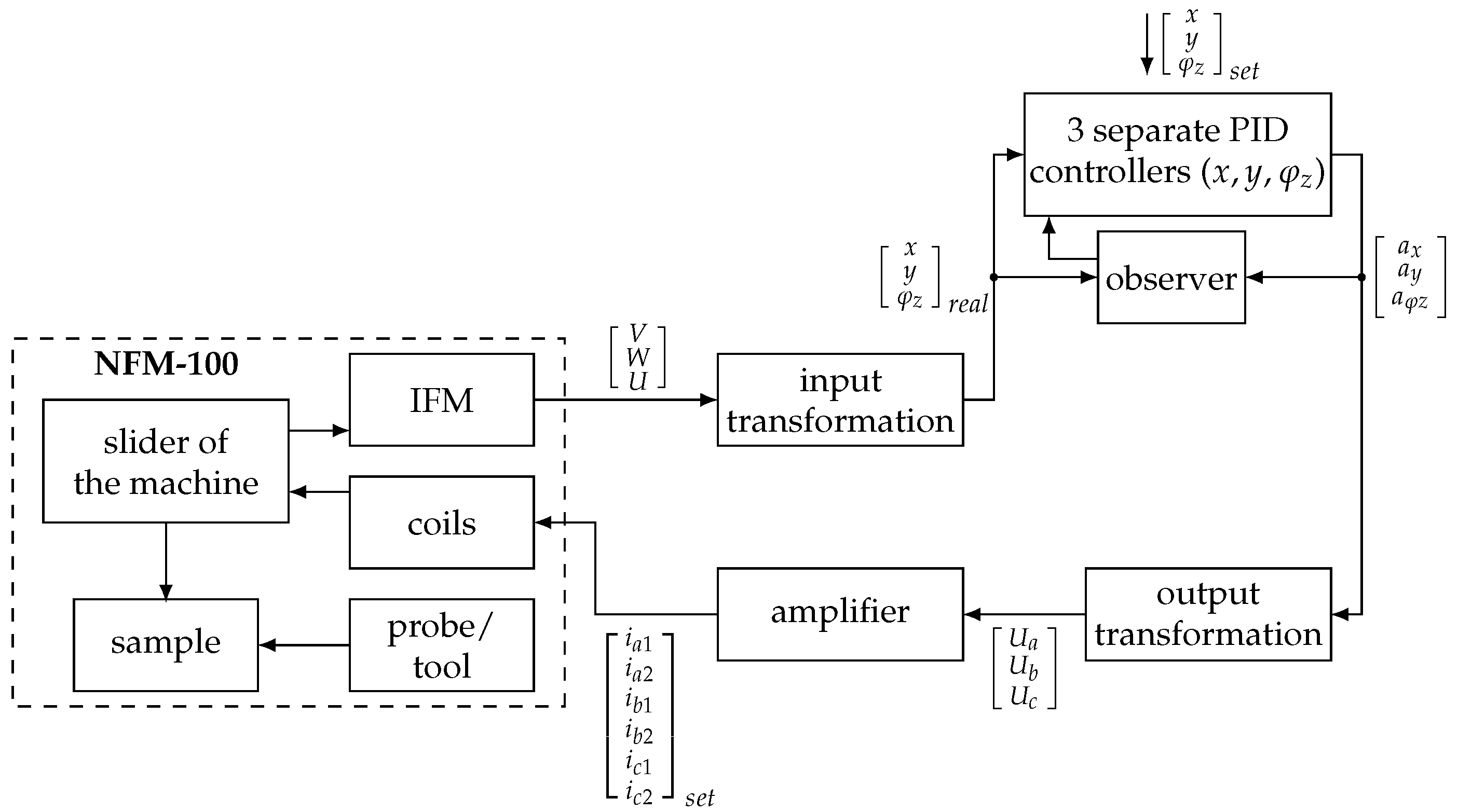
In
Figure 4, the basic structure of the control system is depicted. The measured variables are the three length values of the laser interferometers (
). These are transformed to the positioning coordinates (
). The rotation of the stage around the
z-axis
is calculated from towards the Abbe point symmetrically arranged probe beams of the
U interferometer.
is derived from this separation per angular displacement
. The angular displacement
are kept very small which allows for linearisations of trigonometric functions. Furthermore, the apparent cosine error originating from the distance between origin and
U-mirror (compare
Figure 2) becomes negligible. The implemented simplified reconstruction of the
- and
-axis from the measured length values states as:
where
and
are the rotation angles of the
V and
W axis starting from
x axis.
The core of the control system is formed by three separate classic PID controllers for each of these coordinates [
24]. For
, an independent PID controller in its standard form is employed:
where ⊙ denotes the (element-wise) Hadamard product. Following the notation of
Figure 4, the control error
is thereby given as:
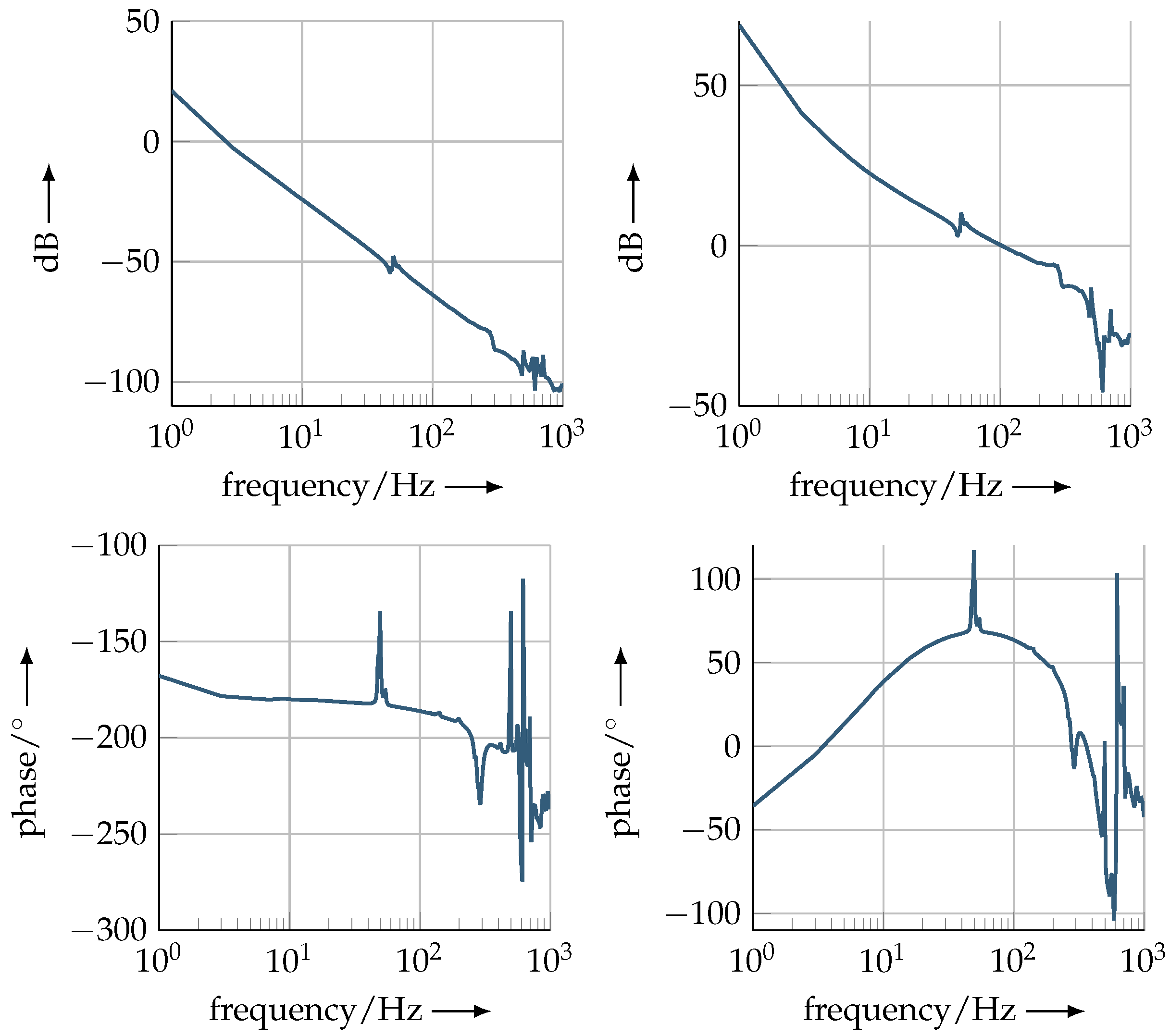
The left side of
Figure 5 shows the reconstructed transfer characteristics of the electromechanical system (plant), including the transformations. There are no significant disturbances in the relevant frequency range up to 50 Hz. The system then can be reduced to a double integrator and small damping term for all movement directions:
where
and
are the state-space variables for each movement direction
. Assuming the mass of the platform
as a well-defined value, the other plant parameters have been found as
for the low-frequency damping constant and
N/A the motor constant. The latter is in well agreement with electromagnetic simulation data, expecting
N/A. The rotational parameters for the
-system can be derived in analogue manner using torques instead of forces.
The PID controller has been designed within the pole-zero plane using the Nyquist stability criterion for each axis individually. The designed gains for Equation (
4) are:
It shall be noted that the integrator has been bounded to limit wind-up. The right side of
Figure 5 shows the resulting open-loop response of the combined controller and plant. At the bandwidth limit at 100 Hz, a phase margin of comfortable
is kept to attain robustness. This is of particular importance, because specimens of different size and weight are frequently changed for examination.
At higher frequencies around
, the plant shows several higher-order resonances of unidentified origin (left side of
Figure 5). To prevent a sensitive reaction of the plant excited by PID controllers at these frequencies, the controller output is supressed through a notch filter from
to
.
Besides its use for the PID design, the model is used to improve the state estimation through an observer. A steady-state Kalman filter will be employed for this purpose. The discrete state-space update equation for the Kalman filter is given for an individual moving direction as [
27]:
where
are the estimates of the states from the measured and transformed noisy movement positions
and the PID controller output acceleration
. The noise co-variances are estimated to be
for the plant and
for the measurement. With these follows an innovation of
and the specific Kalman filter as:
The used interferometers have a sub-nanometre measurement precision. Therefore, only the velocities
shall be estimated by the filter. The lower row for
of this Kalman filter provides this estimation. The velocity of the error therefore follows from Equation (
5) as:
The resulting accelerations from (
4),
, are scaled to currents via their respective motor constants and transformed to the three actuator axes. This actuation transformation differs from the measurement transformation given their different physical domain. For the three drives
, the transformation follows from the
arrangement and the force directions of the coils (compare
Figure 2) as:
These currents are then split onto the two coils depending on their current position-dependent commutation. Magnetic fields of coils and magnets for this commutation are implemented via numerically simulated data.
In the following section, the deviation from the specified trajectory up to the maximum velocity of 20 mm/s is examined after considering the static condition for various movement scenarios.
4. Investigations and Measurement Results
In previous publications, the great potential of the NFM-100 in combination with a tip-based system was shown and statements were made about the accuracy [
5,
10,
11,
17]. In the following part, first, only the machine itself is considered in static operation and, subsequently, its performance at high movement speeds. Furthermore, the deviation from the specified trajectory is analysed for both linear and circular motion.
In the presented setup of the machine, there is no constraint for the x and y direction. Thus, a rotation around the z axis is allowed in principle. Through the use of air bearings, a higher linearity of the x and y movements can be achieved through almost friction- and force-free movement. This is further supported in terms of control technology through precise, permanent measurement and dynamic control of the rotation around the z axis by means of the three voice coil actuators.
Therefore, the position noise of the machine table with a sampling frequency of 10 kHz for a duration of 10 s in the x and y direction as well as the noise of the angle interferometer is first considered. In
Figure 6, the recorded position noise in closed-loop control at the origin is depicted.
The standard deviation (1) of the different values are shown in the following table.
As can be seen in
Table 2, the values fulfil the requirement of an extremely low positioning noise (<1 nm), which is necessary for precise AFM measurements. Moreover, this is especially important for the fabrication of nanostructures, because they cannot be corrected afterwards.
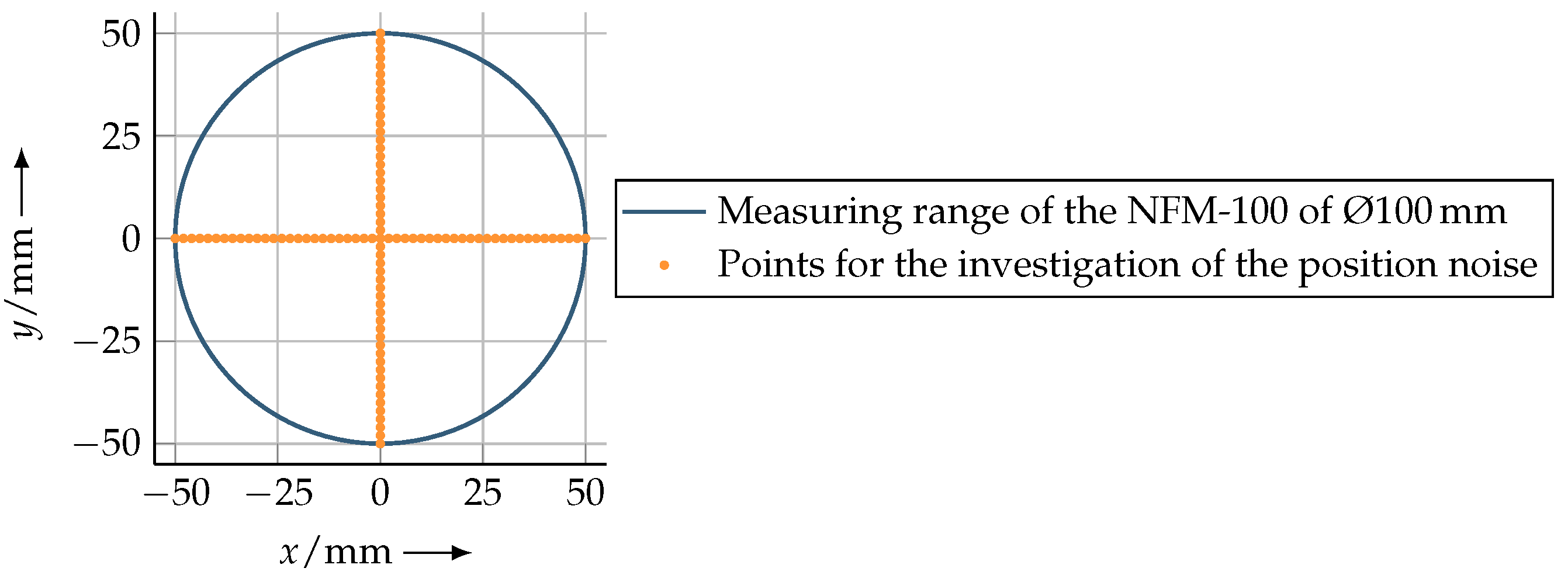
For the further investigation of the static operation, the machine table was moved to several points on the
x and
y axis, where the position noise was recorded.
Figure 7 shows the points where the position noise was recorded within the entire range of motion.
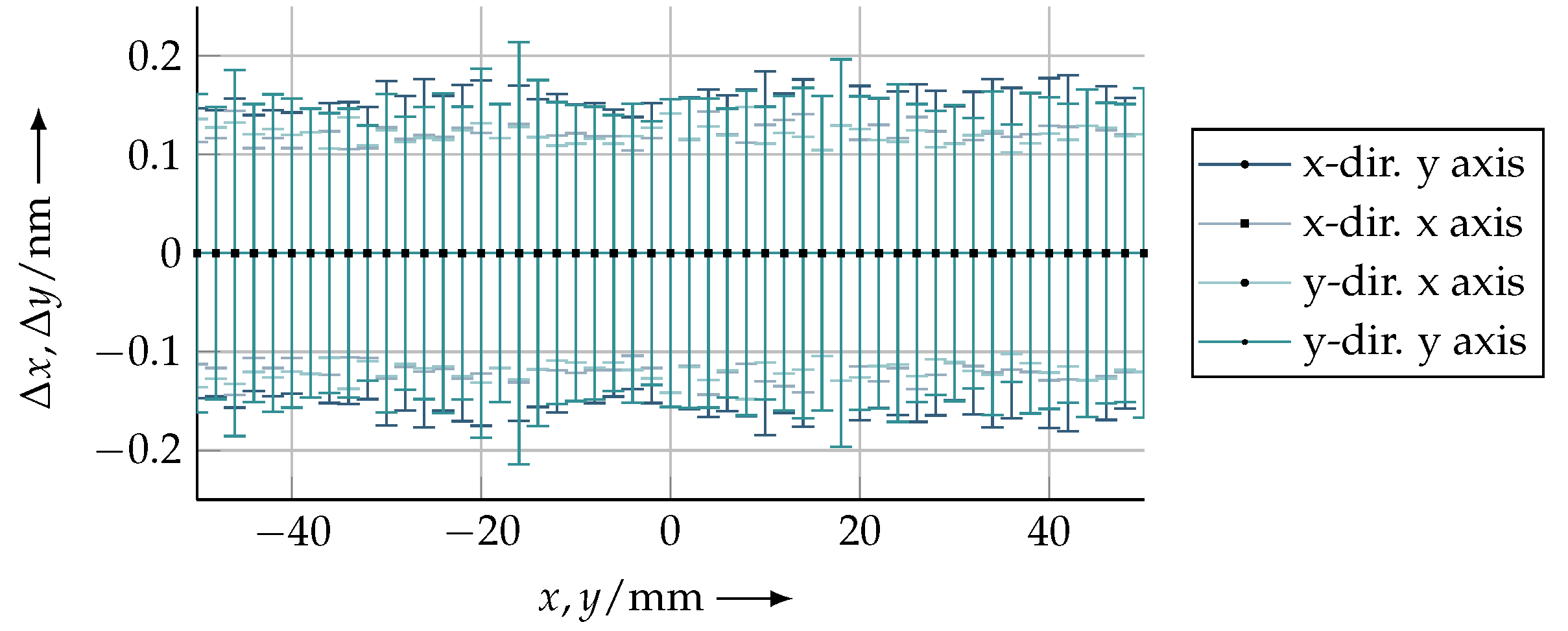
Initially,
Figure 8 shows how the position stability behaves over the movement range of 100 mm in both the
x and
y direction. For this purpose, the position noise was recorded over a period of 10 s with a sampling frequency of 10 kHz, each at a distance of 2 mm on the
x and
y axis over a maximum distance of 100 mm (see
Figure 7). For this purpose, the deviations of the
x and
y axis are plotted in each case.
Over the entire examined range, the maximum deviation is below 450 pm (1
), as can be seen in
Figure 8.
After this static investigation, the focus was placed on the dynamic mode.
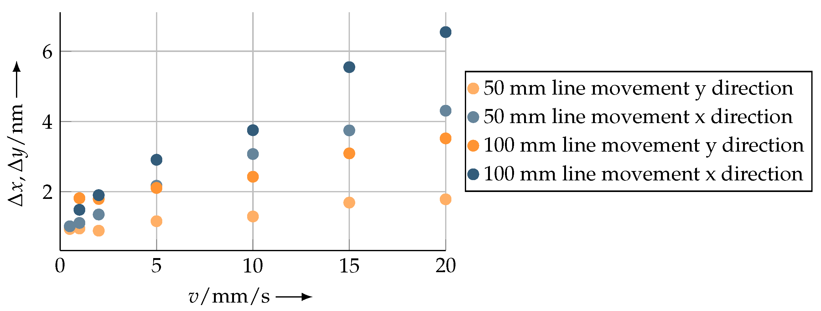
First, straight-line trajectories were driven at different velocities. For this purpose, this analysis was carried out along the
x axis as well as the
y axis over a length of 50 mm and 100 mm. In this case, a velocity range between 0.5 mm/s and 20 mm/s was selected and investigated.
Figure 9 shows that at the maximum velocity of 20 mm/s over a length of 100 mm, the maximum path deviation perpendicular to the moving direction is below 7 nm (6.545 nm).
In addition, it can be seen that the movements in the y direction have a smaller deviation than in the x direction at the same velocity. This can be explained by the fact that when moving in the y direction, two actuators are used equally due to the symmetry of the actuator arrangement. Furthermore, the angular deviation during a line movement with a length of 100 mm at the maximum speed was considered. During line travel in the x direction, an angle deviation (1) of 714 nrad was measured. In the y direction, this measured deviation is 842 nrad.
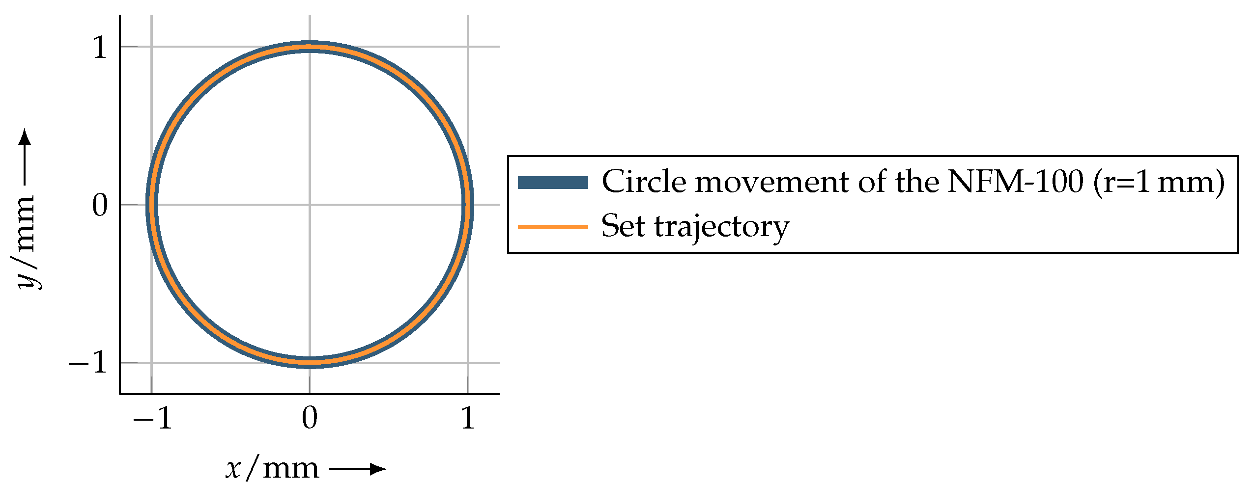
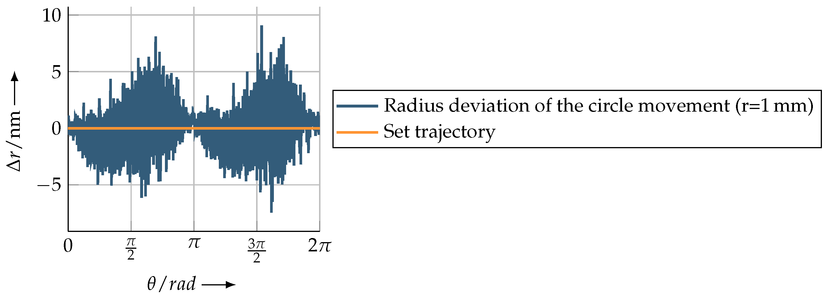
In
Figure 10, five consecutive revolutions with a nominal trajectory with a radius of 1 mm are shown. The movements were carried out at a circumferential velocity of 10 mm/s. In order to illustrate the deviations of the circular path more clearly, the original measurement data were transformed into polar coordinates, which is depicted in the following
Figure 11.
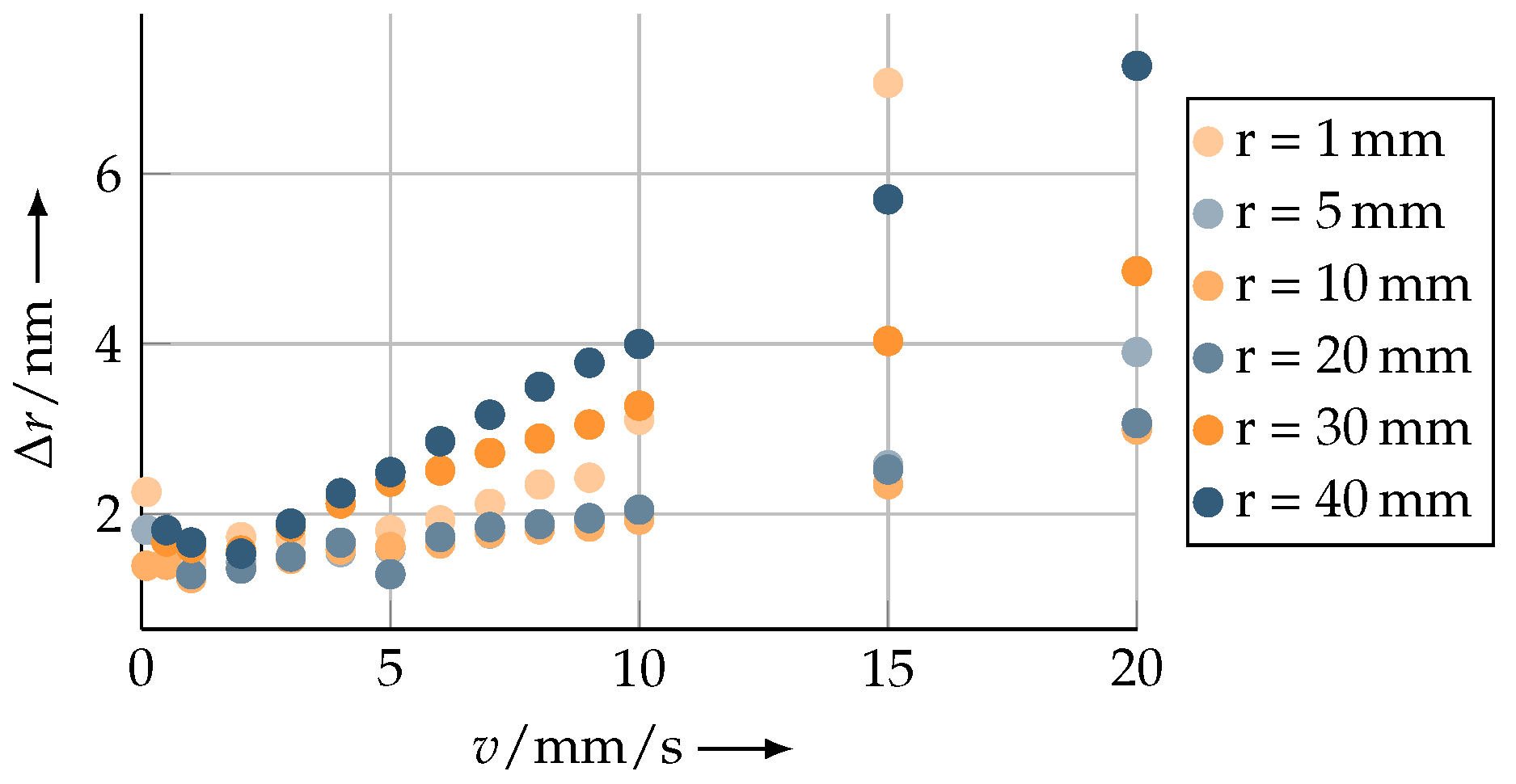
In addition to this investigation,
Figure 12 shows the path deviations of a circular movement as a function of velocity. Different radii were driven with the machine table at various velocities. The examined velocity range was between 0.1 mm/s and 20 mm/s. In this examination, circles with radii between 1 mm and 40 mm were driven at different speeds with five repetitions each. Also in this case, the standard deviation for the radius at the maximum velocity of 20 mm/s at r = 40 mm is 7.269 nm.
For a circular movement with a diameter of 80 mm and a velocity of 20 mm/s, the maximum angular deviation is only 689 nrad.
As mentioned in
Section 3, the selected air bearings are characterised by numerous advantages. However, a residual noise in the
z direction is still present. To investigate this, the existing atomic force microscope (AFM) was used. An AFM scan was made on an area of 10 µm × 10 µm on a sample when the machine table was switched off and, thus, the machine table was directly resting on the granite machine base without an air layer in between. For comparison, a scan was measured when the table was switched on. For this purpose, a sample with a surface that has only very small steps (<1 nm) in the
z direction was selected. Here, a SiC sample was used that has step heights of about 750 pm and step widths between 150 nm and 400 nm. The step height is equal to half of the lattice constant of the 6H-SiC crystal in the [0001] direction [
28]. As shown in
Figure 8, the position noise in the
x and
y direction is below 300 pm, which can be neglected for the AFM scan in that case.
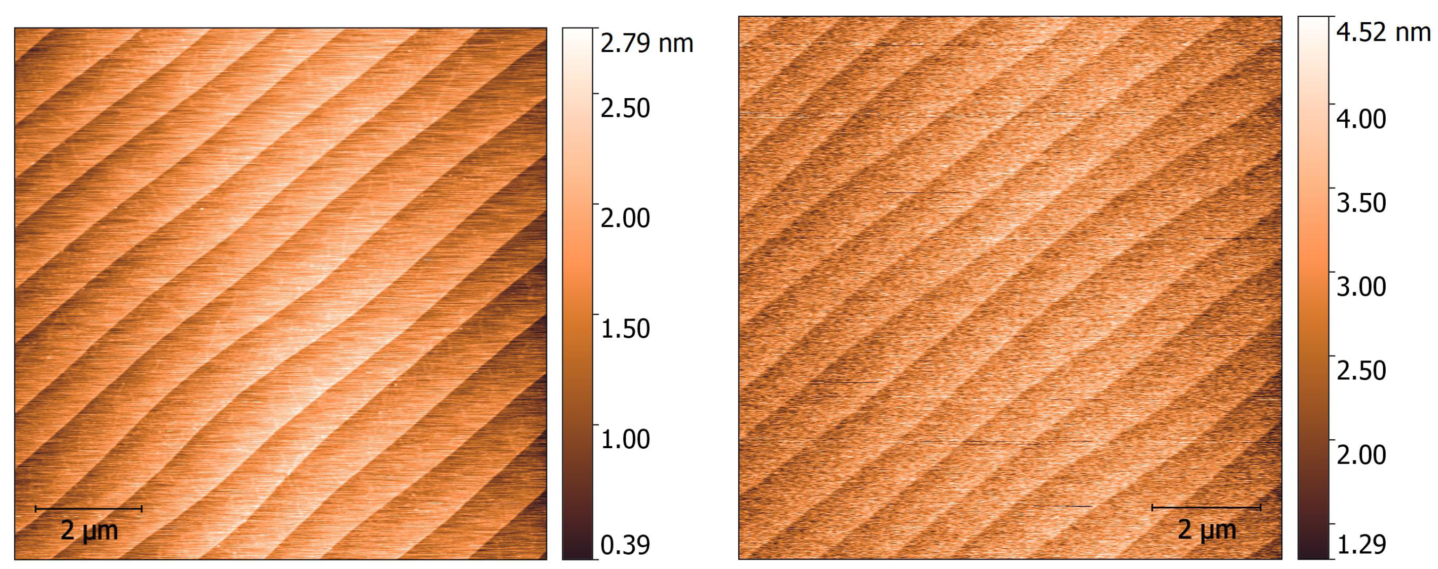
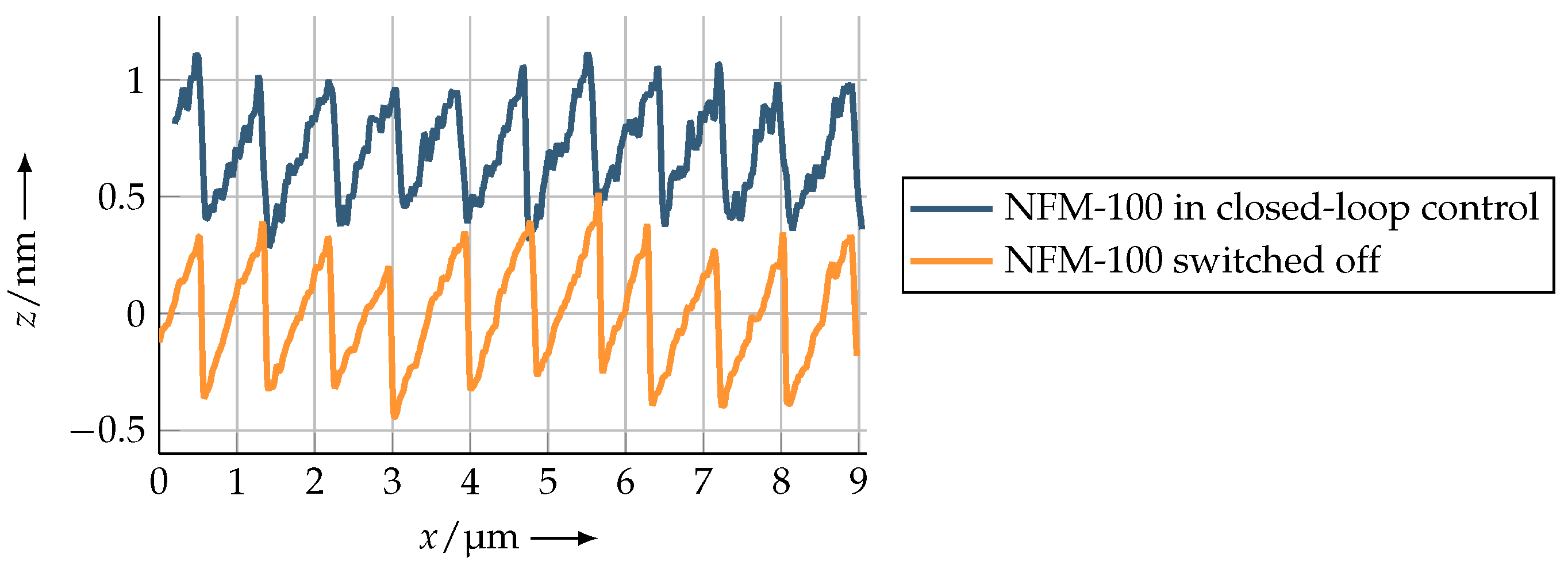
Figure 13 (left and right) shows a topography scan of the aforementioned SiC sample with the difference between the machine table being switched off and on. The scanning speed for both measurements was 5 µm/s.
The individual steps are clearly visible in both pictures. However, in the picture with the machine table switched on, it can be seen that the amount of noise increases slightly.
In addition, a section of the two topography profiles was plotted in
Figure 14 for comparison. The root mean square roughness is only 90 pm for the measurement with the machine table switched off. In contrast, a roughness with the table switched on in closed-loop control was 144 pm.
In general, it can be stated that the influence of the z noise of the setup of the NFM-100 in the range clearly below 1 nm and the AFM measurements are not significantly influenced by the machine table.
In the future, the focus will be on nanofabrication using FESPL. Large-area structures in the form of spirals, circles and lines are to be fabricated and investigated in terms of accuracy and repeatability.


 ,
, 

