
Learning Low-Precision Structured Subnetworks Using Joint Layerwise Channel Pruning and Uniform Quantization


Abstract
:1. Introduction
- We design a greedy layerwise channel pruning strategy using a nonparametric data-driven importance measure built without invoking any distributional assumptions.
- We build a fully data-driven nonparametric framework to learn performant low-precision structured subnetworks by combining our layerwise channel pruning algorithm with quantization-aware training.
- We evaluate our algorithm using alternative pruning schedules and neuron importance measures and demonstrate clear advantages over pre-existing approaches.
- We demonstrate increased performance per memory footprint over existing solutions across a wide range of discriminative and generative computer vision tasks.
2. Background
2.1. Pruning
2.2. Quantization
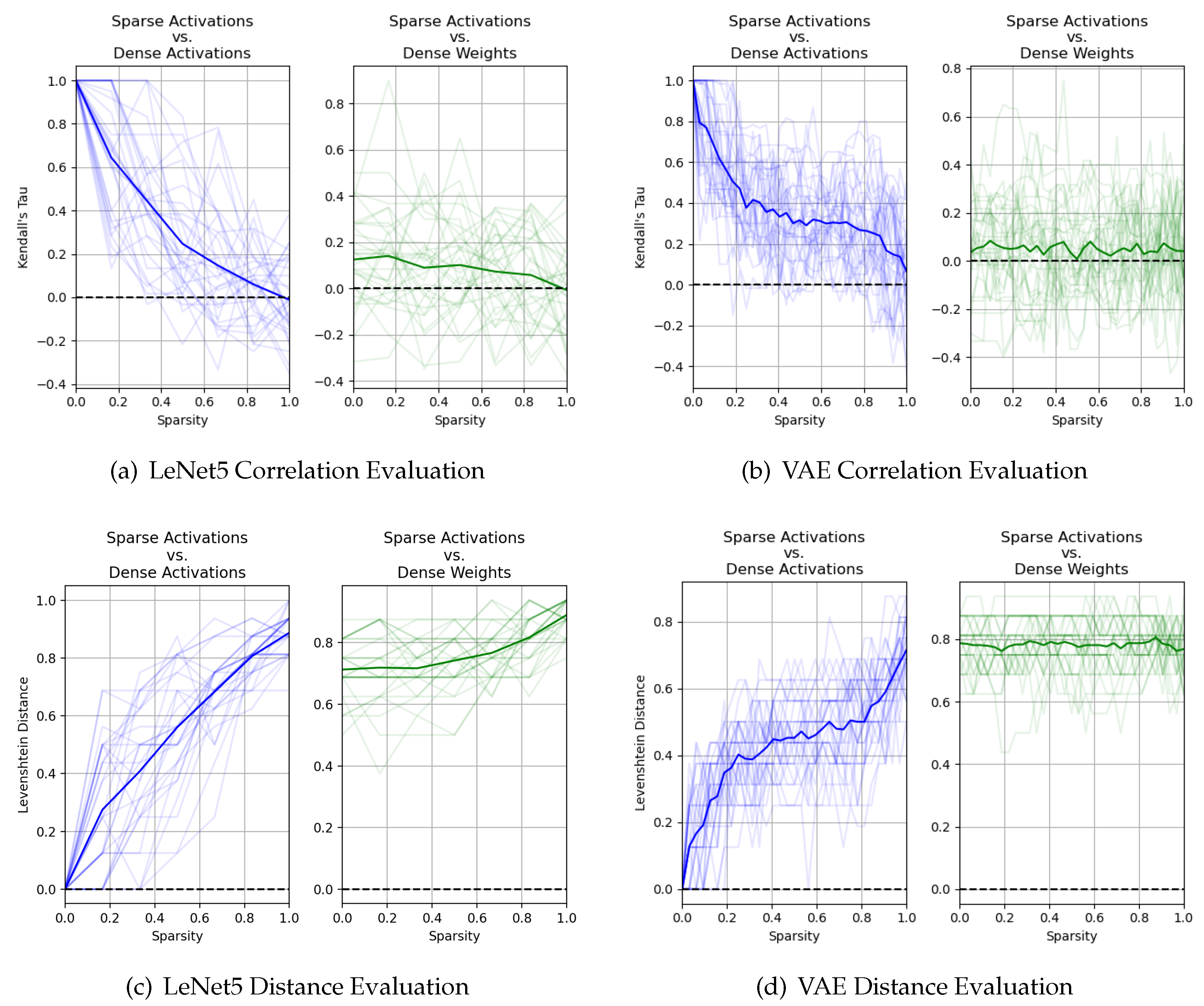
3. Motivation
- Kendall’s Coefficient of Rank Correlation [31]:For a given layer i with outputs channels, let the rank orderings of two sets of importance estimates and be given by and , respectively. The Kendall’s coefficient of rank correlation measures the similarity between and . The statistic (referred to as Kendall’s Tau) is given below in Equation (7), where is given by Equation (8). Here, is a perfect relationship, is no relationship at all, and is a perfect negative relationship.
- Levenshtein Distance [32]:For a given layer i with outputs channels, let the rank orderings of two sets of importance estimates and be given by and , respectively. The Levenshtein distance between these two sequences of ranks, which we denote as , is defined as the minimum number of single element edits required to change to . The distance is formally defined using recursion as given by Equations (9) and (10). The function tail of an ordered set of n elements returns all but the first element of the string such that and tail, where we denote element j of ranked set as . Here, will have a low value close to 0 if and are very similar; otherwise, it will have a high value.
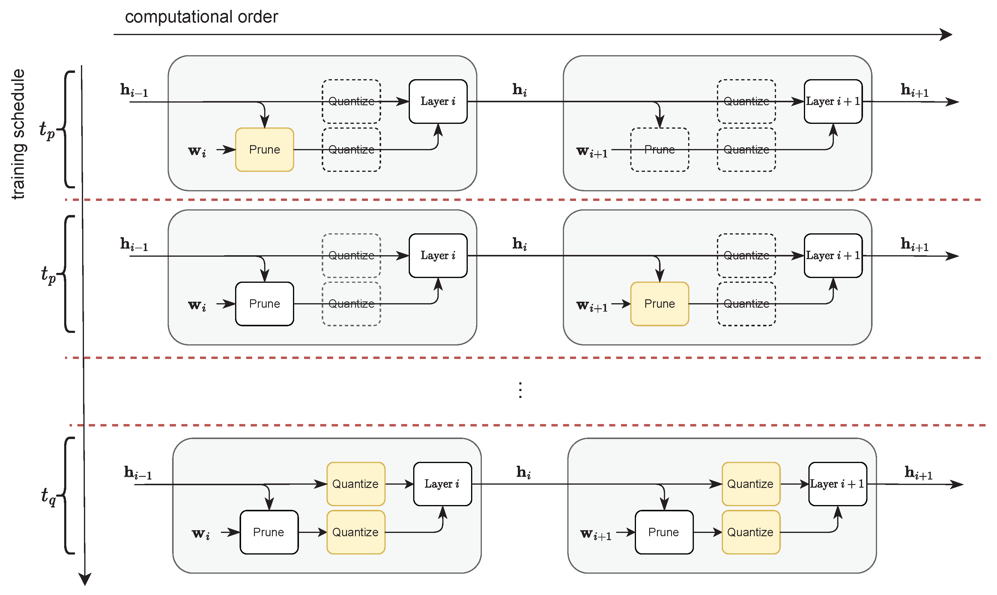
4. Algorithms
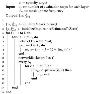
4.1. Greedy Layerwise Channel Pruning Using Nonparametric Statistics
| Algorithm 1: Our proposed layerwise channel pruning algorithm, using per-channel -norm of activations to measure importance. All channel masks are initialized to 1 and all importance measurements are initialized to 0. We update learned weights of all layers in the network at every step using backpropagation, but only update the mask for layer i at step i. |
 |
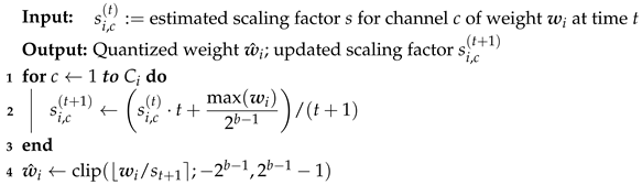
4.2. Uniform Quantization-Aware Training
| Algorithm 2: Our adaptive asymmetric quantization algorithm for our activations using per-tensor scaling factors. We use moving average statistics over hidden activation to estimate the bounds on its dynamic range for the purpose of deriving scaling factor and zero-point for layer i. |
| Input: estimated bounds on hidden activation at time step t Output: Quantized activation ; Updated bounds 1 2 3 4 5 |
| Algorithm 3: Our adaptive symmetric quantization algorithm for the set of weights for layer i using per-channel scaling factors. We use moving average statistics to estimate the maximum weight magnitude for each channel c to derive our per-channel scaling factors . |
 |
5. Experiments
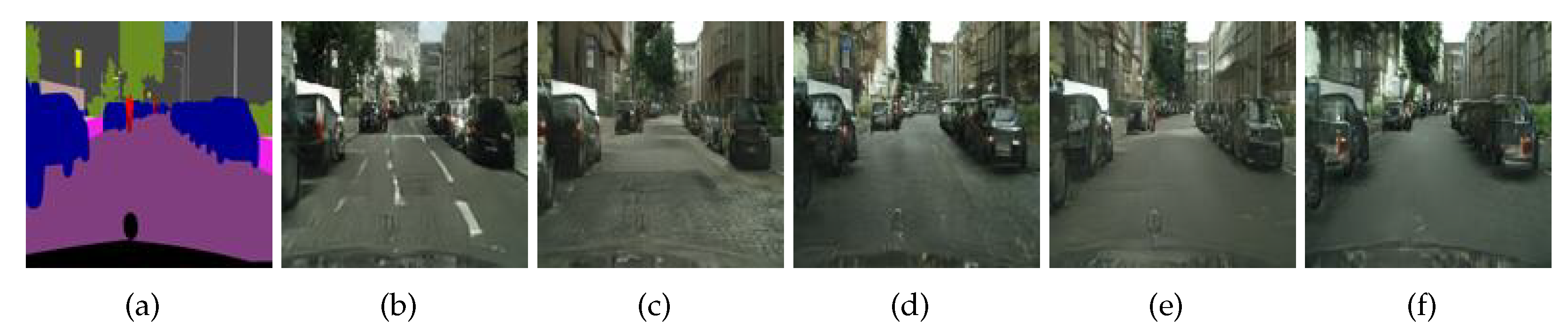
- Image style transfer with CycleGAN [46] on Cityscape
5.1. Evaluating Pruning Schedules and Importance Measures
- Training from scratch. Prior work has demonstrated that, in some cases, there is no need to implement a pruning schedule because pre-defined structured subnetwork architectures can be trained from scratch to match or surpass the performance of the original larger network [38]. As such, we evaluate our pruning algorithm against this baseline.
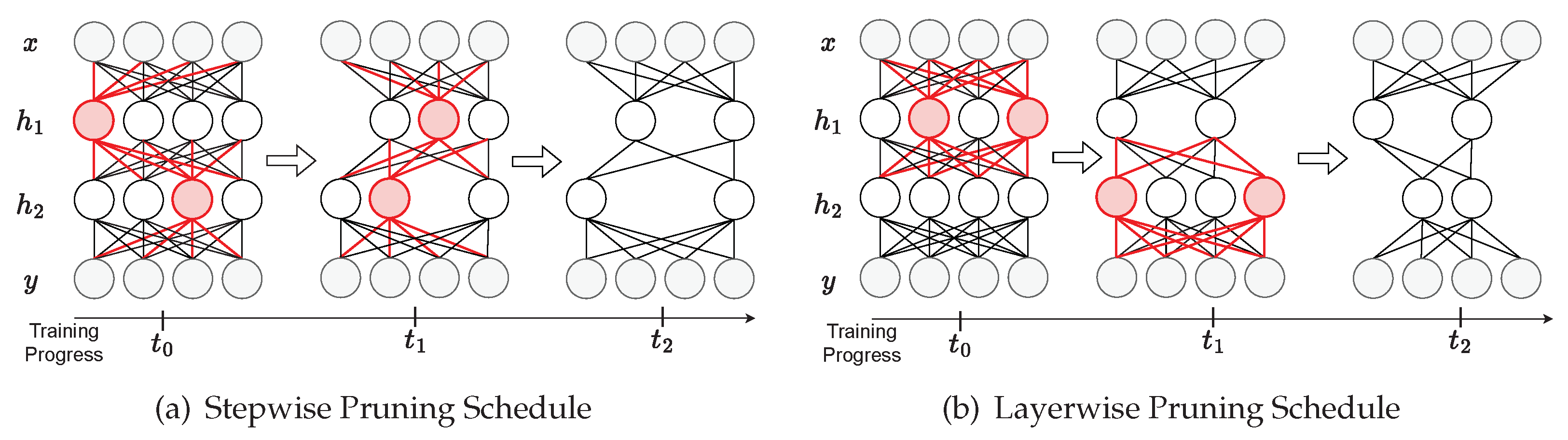
- One-shot. We compare against the common “prune then fine-tune” strategy [20], where we train a fully connected baseline, and then prune the converged model to our target sparsity in one step before fine-tuning to heal the network.
- Stepwise. Unlike one-shot pruning schedules, which jump to the target sparsity in one step, stepwise pruning schedules iteratively increase the sparsity in the network over many steps throughout training. We benchmark against the state-of-the-art iterative pruning schedule proposed by Zhu and Gupta [23].
5.2. Evaluation of Joint Pruning and Quantization
6. Conclusions and Future Work
Author Contributions
Funding
Institutional Review Board Statement
Informed Consent Statement
Data Availability Statement
Acknowledgments
Conflicts of Interest
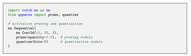
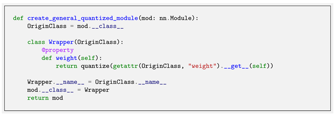
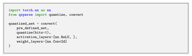
Appendix A. Software Library
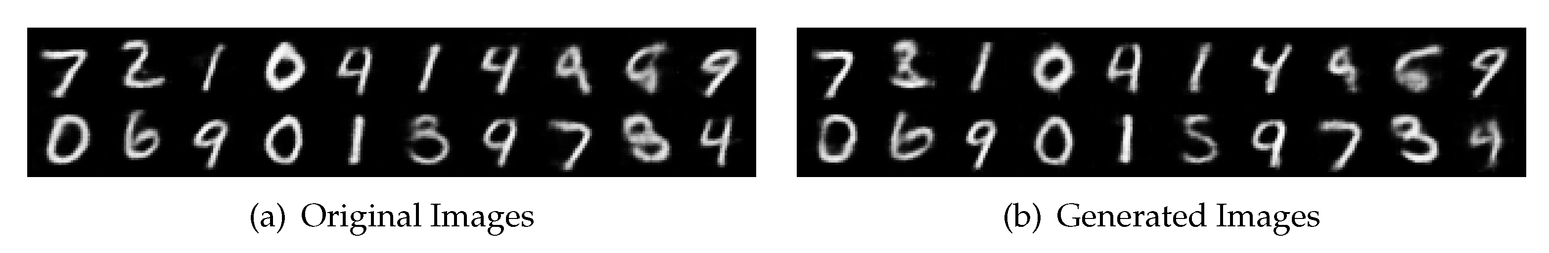
| 1 | We use a network architecture comparable to LeNet for the purpose of a reasonably symmetric evaluation across discriminative and generative tasks. Our encoder uses two convolution layers, each followed by a ReLU and max pooling layer. Our decoder uses three deconvolution layers, each followed by a ReLU except for the final deconvolution layer, which is followed by a sigmoid. |
| 2 | We repeated these experiments using the -norm of the output activations and saw very similar results. |
| 3 | The code for the algorithms discussed in this paper can be found at https://github.com/mlzxy/mdpi202 (accessed on 30 June 2022). |
| 4 | We define operating memory as the aggregate hardware storage area used for weights and activations of the network during inference, all of which are required to be kept so they can be readily accessed. |
References
- Hestness, J.; Narang, S.; Ardalani, N.; Diamos, G.; Jun, H.; Kianinejad, H.; Patwary, M.; Ali, M.; Yang, Y.; Zhou, Y. Deep learning scaling is predictable, empirically. arXiv 2017, arXiv:1712.00409. [Google Scholar]
- Han, S.; Mao, H.; Dally, W.J. Deep Compression: Compressing Deep Neural Network with Pruning, Trained Quantization and Huffman Coding. In Proceedings of the International Conference on Learning Representations, San Juan, Puerto Rico, 2–4 May 2016. [Google Scholar]
- Gale, T.; Elsen, E.; Hooker, S. The state of sparsity in deep neural networks. arXiv 2019, arXiv:1902.09574. [Google Scholar]
- Polino, A.; Pascanu, R.; Alistarh, D. Model compression via distillation and quantization. In Proceedings of the International Conference on Learning Representations, Vancouver, BC, Canada, 30 April–3 May 2018. [Google Scholar]
- Dong, X.; Yang, Y. Network pruning via transformable architecture search. arXiv 2019, arXiv:1905.09717. [Google Scholar]
- Wang, T.; Wang, K.; Cai, H.; Lin, J.; Liu, Z.; Wang, H.; Lin, Y.; Han, S. Apq: Joint search for network architecture, pruning and quantization policy. In Proceedings of the IEEE/CVF Conference on Computer Vision and Pattern Recognition, Seattle, WA, USA, 14–19 June 2020; pp. 2078–2087. [Google Scholar]
- Paupamah, K.; James, S.; Klein, R. Quantisation and pruning for neural network compression and regularisation. In Proceedings of the 2020 International SAUPEC/RobMech/PRASA Conference, Cape Town, South Africa, 29–31 January 2020; pp. 1–6. [Google Scholar]
- Liang, T.; Glossner, J.; Wang, L.; Shi, S.; Zhang, X. Pruning and quantization for deep neural network acceleration: A survey. Neurocomputing 2021, 461, 370–403. [Google Scholar] [CrossRef]
- Zhao, Y.; Gao, X.; Bates, D.; Mullins, R.; Xu, C.Z. Focused quantization for sparse CNNs. arXiv 2019, arXiv:1905.09717. [Google Scholar]
- Yu, P.H.; Wu, S.S.; Klopp, J.P.; Chen, L.G.; Chien, S.Y. Joint Pruning & Quantization for Extremely Sparse Neural Networks. arXiv 2020, arXiv:2010.01892. [Google Scholar]
- Colbert, I.; Kreutz-Delgado, K.; Das, S. AX-DBN: An approximate computing framework for the design of low-power discriminative deep belief networks. In Proceedings of the 2019 International Joint Conference on Neural Networks (IJCNN), Budapest, Hungary, 14–19 July 2019; pp. 1–9. [Google Scholar]
- Van Baalen, M.; Louizos, C.; Nagel, M.; Amjad, R.A.; Wang, Y.; Blankevoort, T.; Welling, M. Bayesian bits: Unifying quantization and pruning. Adv. Neural Inf. Process. Syst. 2020, 33, 5741–5752. [Google Scholar]
- Frankle, J.; Carbin, M. The Lottery Ticket Hypothesis: Finding Sparse, Trainable Neural Networks. In Proceedings of the International Conference on Learning Representations, New Orleans, LA, USA, 6–9 May 2019. [Google Scholar]
- Mao, H.; Han, S.; Pool, J.; Li, W.; Liu, X.; Wang, Y.; Dally, W.J. Exploring the Granularity of Sparsity in Convolutional Neural Networks. In Proceedings of the IEEE Conference on Computer Vision and Pattern Recognition (CVPR) Workshops, Honolulu, HI, USA, 21–26 July 2017. [Google Scholar]
- He, Y.; Zhang, X.; Sun, J. Channel pruning for accelerating very deep neural networks. In Proceedings of the IEEE International Conference on Computer Vision, Honolulu, HI, USA, 21–26 July 2017; pp. 1389–1397. [Google Scholar]
- Jha, N.K.; Mittal, S.; Avancha, S. Data-type aware arithmetic intensity for deep neural networks. Energy 2021, 120, x109. [Google Scholar]
- Colbert, I.; Kreutz-Delgado, K.; Das, S. An Energy-Efficient Edge Computing Paradigm for Convolution-Based Image Upsampling. IEEE Access 2021, 9, 147967–147984. [Google Scholar] [CrossRef]
- Blalock, D.; Gonzalez Ortiz, J.J.; Frankle, J.; Guttag, J. What is the state of neural network pruning? Proc. Mach. Learn. Syst. 2020, 2, 129–146. [Google Scholar]
- Chen, T.; Chen, X.; Ma, X.; Wang, Y.; Wang, Z. Coarsening the Granularity: Towards Structurally Sparse Lottery Tickets. In Proceedings of the International Conference on Machine Learning, Baltimore, MA, USA, 17–23 July 2022. [Google Scholar]
- Hu, H.; Peng, R.; Tai, Y.W.; Tang, C.K. Network trimming: A data-driven neuron pruning approach towards efficient deep architectures. arXiv 2016, arXiv:1607.03250. [Google Scholar]
- Dai, B.; Zhu, C.; Guo, B.; Wipf, D. Compressing neural networks using the variational information bottleneck. In Proceedings of the International Conference on Machine Learning. PMLR, 2018, Stockholm, Sweden, 10–15 July 2018; pp. 1135–1144. [Google Scholar]
- Molchanov, P.; Mallya, A.; Tyree, S.; Frosio, I.; Kautz, J. Importance estimation for neural network pruning. In Proceedings of the IEEE/CVF Conference on Computer Vision and Pattern Recognition, Long Beach, CA, USA, 15–20 June 2019; pp. 11264–11272. [Google Scholar]
- Zhu, M.; Gupta, S. To Prune, or Not to Prune: Exploring the Efficacy of Pruning for Model Compression. In Proceedings of the International Conference on Learning Representations, Vancouver, BC, Canada, 30 April–3 May 2018. [Google Scholar]
- Luo, J.H.; Wu, J.; Lin, W. Thinet: A filter level pruning method for deep neural network compression. In Proceedings of the IEEE International Conference on Computer Vision, Honolulu, HI, USA, 21–26 July 2017; pp. 5058–5066. [Google Scholar]
- Wang, Y.; Lu, Y.; Blankevoort, T. Differentiable joint pruning and quantization for hardware efficiency. In Proceedings of the European Conference on Computer Vision, Glasgow, UK, 23–28 August 2020; Springer: Cham, Switzerland, 2020; pp. 259–277. [Google Scholar]
- Wu, H.; Judd, P.; Zhang, X.; Isaev, M.; Micikevicius, P. Integer Quantization for Deep Learning Inference: Principles and Empirical Evaluation. arXiv 2020, arXiv:2004.09602. [Google Scholar]
- Jacob, B.; Kligys, S.; Chen, B.; Zhu, M.; Tang, M.; Howard, A.; Adam, H.; Kalenichenko, D. Quantization and training of neural networks for efficient integer-arithmetic-only inference. In Proceedings of the IEEE Conference on Computer Vision and Pattern Recognition, Salt Lake City, UT, USA, 18–23 June 2018; pp. 2704–2713. [Google Scholar]
- Krishnamoorthi, R. Quantizing deep convolutional networks for efficient inference: A whitepaper. arXiv 2018, arXiv:1806.08342. [Google Scholar]
- Gholami, A.; Kim, S.; Dong, Z.; Yao, Z.; Mahoney, M.W.; Keutzer, K. A survey of quantization methods for efficient neural network inference. arXiv 2021, arXiv:1806.08342. [Google Scholar]
- Jain, S.; Gural, A.; Wu, M.; Dick, C. Trained quantization thresholds for accurate and efficient fixed-point inference of deep neural networks. Proc. Mach. Learn. Syst. 2020, 2, 112–128. [Google Scholar]
- Knight, W.R. A computer method for calculating Kendall’s tau with ungrouped data. J. Am. Stat. Assoc. 1966, 61, 436–439. [Google Scholar] [CrossRef]
- Levenshtein, V.I. Binary codes capable of correcting deletions, insertions, and reversals. In Soviet Physics—Doklady; 1966; Volume 10, pp. 707–710. Available online: https://nymity.ch/sybilhunting/pdf/Levenshtein1966a.pdf (accessed on 30 June 2022).
- LeCun, Y.; Bottou, L.; Bengio, Y.; Haffner, P. Gradient-based learning applied to document recognition. Proc. IEEE 1998, 86, 2278–2324. [Google Scholar] [CrossRef] [Green Version]
- LeCun, Y. The MNIST Database of Handwritten Digits. 1998. Available online: http://yann.lecun.com/exdb/mnist/ (accessed on 30 June 2022).
- Heusel, M.; Ramsauer, H.; Unterthiner, T.; Nessler, B.; Hochreiter, S. Gans trained by a two time-scale update rule converge to a local nash equilibrium. Adv. Neural Inf. Process. Syst. 2017, 30. [Google Scholar]
- Tishby, N.; Zaslavsky, N. Deep learning and the information bottleneck principle. In Proceedings of the 2015 IEEE information theory workshop (itw), Jerusalem, Israel, 26 April–1 May 2015; pp. 1–5. [Google Scholar]
- He, K.; Zhang, X.; Ren, S.; Sun, J. Deep residual learning for image recognition. In Proceedings of the IEEE Conference on Computer Vision and Pattern Recognition, Las Vegas, NV, USA, 27–20 June 2016; pp. 770–778. [Google Scholar]
- Liu, Z.; Sun, M.; Zhou, T.; Huang, G.; Darrell, T. Rethinking the Value of Network Pruning. In Proceedings of the International Conference on Learning Representations, New Orleans, LA, USA, 6–9 May 2019. [Google Scholar]
- Bengio, Y.; Léonard, N.; Courville, A. Estimating or propagating gradients through stochastic neurons for conditional computation. arXiv 2013, arXiv:1308.3432. [Google Scholar]
- Huang, G.; Liu, Z.; Van Der Maaten, L.; Weinberger, K.Q. Densely connected convolutional networks. In Proceedings of the IEEE Conference on Computer Vision and Pattern Recognition (CVPR) Workshops, Honolulu, HI, USA, 21–26 July 2017; pp. 4700–4708. [Google Scholar]
- Sandler, M.; Howard, A.; Zhu, M.; Zhmoginov, A.; Chen, L.C. Mobilenetv2: Inverted residuals and linear bottlenecks. In Proceedings of the International Conference on Machine Learning, PMLR, 2018, Stockholm, Sweden, 10–15 July 2018; pp. 4510–4520. [Google Scholar]
- Krizhevsky, A.; Hinton, G. Learning Multiple Layers of Features from Tiny Images. 2009. Available online: https://www.cs.toronto.edu/~kriz/learning-features-2009-TR.pdf (accessed on 30 June 2022).
- Ronneberger, O.; Fischer, P.; Brox, T. U-net: Convolutional networks for biomedical image segmentation. In Proceedings of the International Conference on Medical image computing and computer-assisted intervention, Munich, Germany, 5–9 October 2015; Springer: Berlin/Heidelberg, Germany, 2015; pp. 234–241. [Google Scholar]
- Pohlen, T.; Hermans, A.; Mathias, M.; Leibe, B. Full-resolution residual networks for semantic segmentation in street scenes. In Proceedings of the IEEE Conference on Computer Vision and Pattern Recognition (CVPR) Workshops, Honolulu, HI, USA, 21—26 July 2017; pp. 4151–4160. [Google Scholar]
- Cordts, M.; Omran, M.; Ramos, S.; Rehfeld, T.; Enzweiler, M.; Benenson, R.; Franke, U.; Roth, S.; Schiele, B. The Cityscapes Dataset for Semantic Urban Scene Understanding. In Proceedings of the IEEE Conference on Computer Vision and Pattern Recognition (CVPR), Las Vegas, NV, USA, 27–30 June 2016. [Google Scholar]
- Zhu, J.Y.; Park, T.; Isola, P.; Efros, A.A. Unpaired image-to-image translation using cycle-consistent adversarial networks. In Proceedings of the IEEE Conference on Computer Vision and Pattern Recognition (CVPR) Workshops, Honolulu, HI, USA; pp. 2223–2232.
- Paszke, A.; Gross, S.; Massa, F.; Lerer, A.; Bradbury, J.; Chanan, G.; Killeen, T.; Lin, Z.; Gimelshein, N.; Antiga, L.; et al. Pytorch: An imperative style, high-performance deep learning library. Adv. Neural Inf. Process. Syst. 2019, 32, 8026–8037. [Google Scholar]
- Nautilus. 2022. Available online: https://ucsd-prp.gitlab.io/ (accessed on 30 June 2022).
- Thomas, M.M.; Vaidyanathan, K.; Liktor, G.; Forbes, A.G. A reduced-precision network for image reconstruction. ACM Trans. Graph. Tog 2020, 39, 1–12. [Google Scholar] [CrossRef]
- Rezk, N.M.; Nordström, T.; Ul-Abdin, Z. Shrink and Eliminate: A Study of Post-Training Quantization and Repeated Operations Elimination in RNN Models. Information 2022, 13, 176. [Google Scholar] [CrossRef]
- Yang, H.; Gui, S.; Zhu, Y.; Liu, J. Automatic neural network compression by sparsity-quantization joint learning: A constrained optimization-based approach. In Proceedings of the IEEE/CVF Conference on Computer Vision and Pattern Recognition, Seattle, WA, USA, 13–19 June 2020; pp. 2178–2188. [Google Scholar]
- Zhang, X. A Design Methodology for Efficient Implementation of Deconvolutional Neural Networks on an FPGA; University of California: San Diego, CA, USA, 2017. [Google Scholar]
- Biookaghazadeh, S.; Zhao, M.; Ren, F. Are {FPGAs} Suitable for Edge Computing? In Proceedings of the USENIX Workshop on Hot Topics in Edge Computing (HotEdge 18), Boston, MA, USA, 10 July 2018. [Google Scholar]
- Colbert, I.; Daly, J.; Kreutz-Delgado, K.; Das, S. A competitive edge: Can FPGAs beat GPUs at DCNN inference acceleration in resource-limited edge computing applications? arXiv 2021, arXiv:2102.00294. [Google Scholar]
- Choi, Y.; El-Khamy, M.; Lee, J. Towards the Limit of Network Quantization. In Proceedings of the International Conference on Learning Representations, oulon, France, 24–26 April 2017. [Google Scholar]
- Achterhold, J.; Koehler, J.M.; Schmeink, A.; Genewein, T. Variational network quantization. In Proceedings of the International Conference on Learning Representations, Vancouver, BC, Canada, 30 April–3 May 2018. [Google Scholar]
- Zhao, C.; Ni, B.; Zhang, J.; Zhao, Q.; Zhang, W.; Tian, Q. Variational convolutional neural network pruning. In Proceedings of the IEEE/CVF Conference on Computer Vision and Pattern Recognition, Long Beach, CA, USA, 15–20 June 2019; pp. 2780–2789. [Google Scholar]
- Xiao, X.; Wang, Z. Autoprune: Automatic network pruning by regularizing auxiliary parameters. Adv. Neural Inf. Process. Syst. (NeurIPS 2019) 2019, 32. [Google Scholar]
- Dettmers, T.; Zettlemoyer, L. Sparse networks from scratch: Faster training without losing performance. arXiv 2019, arXiv:1907.04840. [Google Scholar]
- Paupamah, K.; James, S.; Klein, R. Quantisation and pruning for neural network compression and regularisation. In Proceedings of the 2020 International SAUPEC/RobMech/PRASA Conference, Cape Town, South Africa, 29–31 January 2020; pp. 1–6. [Google Scholar]
- Choi, Y.; El-Khamy, M.; Lee, J. Universal deep neural network compression. IEEE J. Sel. Top. Signal Process. 2020, 14, 715–726. [Google Scholar] [CrossRef] [Green Version]
- Pappalardo, A. Xilinx/Brevitas. Available online: https://zenodo.org/record/5779154#.YujQyepBxPY (accessed on 30 June 2022).
- torch.nn.qat — PyTorch 1.9.0 Documentation. 2021. Available online: https://pytorch.org/docs/stable/torch.nn.qat.html (accessed on 30 June 2022).
- Coelho, C.N., Jr.; Kuusela, A.; Zhuang, H.; Aarrestad, T.; Loncar, V.; Ngadiuba, J.; Pierini, M.; Summers, S. Ultra low-latency, low-area inference accelerators using heterogeneous deep quantization with QKeras and hls4ml. arXiv 2020, arXiv:2006.10159. [Google Scholar]


| Classification (Accuracy) | Segmentation (mIOU) | Style Transfer (FID) | ||||
|---|---|---|---|---|---|---|
| DenseNet121 | MobileNetV2 | UNet | FRRNet | CycleGAN | ||
| Baseline | Full Model | 78.70 | 68.31 | 61.69 | 66.32 | 47.17 |
| 50% Sparsity | From Scratch | 76.75 | 65.36 | 58.90 | 61.84 | 50.39 |
| One-Shot | 78.40 | 67.39 | 60.59 | 64.53 | 49.43 | |
| Stepwise | 77.14 | 68.05 | 58.13 | 64.90 | 52.83 | |
| Layerwise (Ours) | 78.77 | 67.58 | 60.57 | 65.52 | 48.06 | |
| 75% Sparsity | From Scratch | 73.07 | 56.66 | 56.71 | 59.29 | 59.55 |
| One-Shot | 76.40 | 56.16 | 52.77 | 58.71 | 57.07 | |
| Stepwise | 72.55 | 60.40 | 51.05 | 56.59 | 65.67 | |
| Layerwise (Ours) | 76.44 | 60.71 | 56.48 | 61.14 | 55.48 | |
| Classification (Accuracy) | Segmentation (mIOU) | Style Transfer (FID) | ||||
|---|---|---|---|---|---|---|
| DenseNet121 | MobileNetV2 | UNet | FRRNet | CycleGAN | ||
| Baseline | Full Model | 78.70 | 68.31 | 61.69 | 66.32 | 47.17 |
| 50% Sparsity | Layerwise (A) | 78.77 | 67.58 | 60.57 | 65.52 | 48.06 |
| Layerwise (W) | 77.88 | 67.56 | 59.41 | 66.16 | 52.52 | |
| 75% Sparsity | Layerwise (A) | 76.44 | 60.71 | 56.48 | 61.14 | 55.48 |
| Layerwise (W) | 73.53 | 60.62 | 54.38 | 60.18 | 67.97 | |
| Classification (Accuracy) | Segmentation (mIOU) | Style Transfer (FID) | ||||
|---|---|---|---|---|---|---|
| DenseNet121 | MobileNetV2 | UNet | FRRNet | CycleGAN | ||
| Baseline | Full Model | 78.70 | 68.31 | 61.69 | 66.32 | 47.17 |
| W8A8 | 79.04 | 68.26 | 62.03 | 66.43 | 49.89 | |
| 50% Sparsity | W8A8 | 79.01 | 67.58 | 60.44 | 64.81 | 58.12 |
| W4A8 | 78.41 | 64.67 | 60.15 | 63.42 | 64.25 | |
| W4A4 | 75.99 | 59.25 | 56.12 | 59.04 | 92.71 | |
| 75% Sparsity | W8A8 | 76.17 | 61.02 | 56.15 | 61.28 | 85.89 |
| W4A8 | 76.12 | 55.41 | 55.60 | 60.90 | 92.12 | |
| W4A4 | 73.62 | 49.49 | 51.90 | 54.16 | 119.19 | |
| Method | Network | Baseline Acc | Accuracy | Weights (Mb) | Activations (Mb) | PD (Acc/Mb) | ||||
|---|---|---|---|---|---|---|---|---|---|---|
| [55] | ResNet-32 | 8 | – | 77.8% | – | 92.58 | 92.64 (+0.06) | 0.83 | 20.19 | 4.41 |
| [56] | DenseNet-76 | 2 | – | 54% | – | 92.19 | 91.17 (−1.02) | 0.68 | 141.26 | 0.64 |
| [38] | VGG-19 | – | – | 95% | – | 93.50 | 93.34 (−0.16) | 16.03 | 19.40 | 2.63 |
| PreResNet-110 | – | – | 95% | – | 95.04 | 92.35 (−2.69) | 1.38 | 67.50 | 1.34 | |
| DenseNet-100 | – | – | 95% | – | 95.24 | 94.19 (−1.05) | 0.97 | 213.37 | 0.44 | |
| VGG-19 | – | – | 70% | 70% | 93.5 | 93.60 (+0.1) | 70.70 | 5.31 | 1.23 | |
| PreResNet-164 | – | – | 60% | 60% | 95.04 | 94.23 (−0.81) | 16.67 | 40.21 | 1.66 | |
| DenseNet-40 | – | – | 60% | 60% | 94.10 | 93.87 (−0.23) | 1.60 | 22.97 | 3.82 | |
| [57] | DenseNet-40 | – | – | 60% | 60% | 94.11 | 93.16 (−0.95) | 1.60 | 22.97 | 3.79 |
| ResNet-20 | – | – | 38% | 38% | 92.01 | 91.66 (−0.35) | 2.70 | 7.96 | 8.59 | |
| ResNet-56 | – | – | 45% | 45% | 93.04 | 92.26 (−0.78) | 7.53 | 19.18 | 3.45 | |
| ResNet-110 | – | – | 63% | 63% | 93.21 | 92.96 (−0.25) | 10.25 | 25.12 | 2.63 | |
| [58] | VGG-16 | – | – | 78.8% | 78.8% | 93.40 | 91.50 (−1.90) | 49.96 | 3.75 | 1.70 |
| [59] | VGG16-C | – | – | 95% | – | 93.51 | 93.00 (−0.51) | 11.78 | 17.70 | 3.15 |
| WRN-22-8 | – | – | 95% | – | 95.74 | 95.07 (−0.67) | 13.73 | 115.34 | 0.74 | |
| [51] | ResNet-20 | 1.9 | – | 54% | – | 91.29 | 91.15 (−0.14) | 0.24 | 12.85 | 6.97 |
| [12] | VGG-7 | 4.8 | 5.4 | – | – | 93.05 | 93.23 (+0.18) | 43.85 | 3.27 | 1.98 |
| [60] | MobileNet | 8 | 8 | – | – | 91.31 | 90.59 (−0.72) | 25.74 | 13.17 | 2.33 |
| [61] | ResNet-32 | 8 | – | 87.5% | – | 92.58 | 92.57 (−0.01) | 0.47 | 20.19 | 4.48 |
| Ours | ResNet-32 | 8 | 8 | 25% | 25% | 92.58 | 92.53 − | 2.80 | 7.57 | 8.92 |
| 8 | 8 | 40% | 40% | 91.77 (−0.81) | 2.24 | 6.06 | 11.06 | |||
| 8 | 8 | 50% | 50% | 90.16 (−2.42) | 1.87 | 5.05 | 13.04 | |||
| 4 | 4 | 50% | 50% | 87.30 (−5.28) | 0.93 | 2.52 | 25.25 |
Publisher’s Note: MDPI stays neutral with regard to jurisdictional claims in published maps and institutional affiliations. |
© 2022 by the authors. Licensee MDPI, Basel, Switzerland. This article is an open access article distributed under the terms and conditions of the Creative Commons Attribution (CC BY) license (https://creativecommons.org/licenses/by/4.0/).
Share and Cite
Zhang, X.; Colbert, I.; Das, S. Learning Low-Precision Structured Subnetworks Using Joint Layerwise Channel Pruning and Uniform Quantization. Appl. Sci. 2022, 12, 7829. https://doi.org/10.3390/app12157829
Zhang X, Colbert I, Das S. Learning Low-Precision Structured Subnetworks Using Joint Layerwise Channel Pruning and Uniform Quantization. Applied Sciences. 2022; 12(15):7829. https://doi.org/10.3390/app12157829
Chicago/Turabian StyleZhang, Xinyu, Ian Colbert, and Srinjoy Das. 2022. "Learning Low-Precision Structured Subnetworks Using Joint Layerwise Channel Pruning and Uniform Quantization" Applied Sciences 12, no. 15: 7829. https://doi.org/10.3390/app12157829
APA StyleZhang, X., Colbert, I., & Das, S. (2022). Learning Low-Precision Structured Subnetworks Using Joint Layerwise Channel Pruning and Uniform Quantization. Applied Sciences, 12(15), 7829. https://doi.org/10.3390/app12157829