1. Introduction
In recent years, machine learning models have been widely adopted in edge devices. Applying these models to resource-constrained hardware has accelerated research into the design of both computationally efficient neural network models and specialized hardware accelerators that are optimized to execute these neural networks. Many compact neural networks for mobile deployment have been designed, but optimal performance for a given hardware platform can only be achieved when the network is co-designed for it—not every model design choice that aims to improve efficiency does so on every hardware platform.
However, designing neural networks that can run on a certain target platform with a target latency is a complex task as there are many design choices, ranging from the type of layers used to the spatial resolution and the channel width of each block. Early work was carried out by manually designing efficient networks. MobileNetV1 [
1] and its introduction of depthwise separable convolutions stimulated the beginning of a research field focused on the design of efficient vision models that can be deployed on embedded and mobile platforms. Subsequently, improved model architectures were released: MobileNetV2 [
2] adds inverted residuals and inverted bottlenecks and MobileNetV3 [
3] expands this further by adding a squeeze-and-excitation module [
4] to the bottleneck structure. Another family of efficient models based on group convolutions and a shuffle operator are the ShuffleNets [
5,
6]. All these models use multi-layer
building blocks that are repeated multiple times in the network. Their design process focuses mainly on optimising the layer structure of the building blocks to make them hardware efficient. Different variations of a network are typically manually designed [
6,
7,
8], or scaled using a single complexity parameter to trade-off between task performance (e.g., accuracy) and computational cost, e.g., input resolution or channel width [
1,
6].
In order to compare such efficient models, most studies have used curve estimates that show the trade-off between accuracy and a model complexity metric, such as FLOPs or latency, for predefined model variants of a model family. These curves allow practitioners to gain insight into these trade-offs and make the best choices for their design constraints. The problem with curve-based comparisons is that they only use a handful of model variants, while each model type still has a very large number of hyperparameters. Once the initial mobile building blocks had been established, the design process, therefore, shifted towards neural architecture search to find new state-of-the-art efficient models. Networks optimized with NAS have repeatedly been shown to outperform manually designed networks [
9,
10,
11,
12,
13]. As efficient models are targeted towards mobile and embedded platforms, they are often resource-constrained. Hardware-aware NAS incorporates these constraints into the search, which enables the finding of optimal models for specific target platforms [
14,
15,
16,
17]. However, the effectiveness of NAS comes with the very large computational cost of training and evaluating many candidate networks. A truly wide search is only feasible when large budgets can be spent on computing resources. For this reason, in practice, the search space of current NAS methods is usually constrained using techniques such as parameter sharing [
13]. These so called one-shot NAS approaches amortize the training cost of all networks in the search space by training all possible architectures together in a large supernet, reducing the cost of NAS by several orders of magnitude [
18]. As a result most approaches in NAS now use a search space with a single fixed building block while searching for other important parameters, such as network depth and width or kernel filter size. The choice of the layer structure within the building block itself is mostly based on the literature, common practice or previous experience.
As we will show, the relative efficiency of network families that use different building blocks depends on both the architecture of the targeted hardware platform and on the desired accuracy range. This means that a true hardware-aware network design approach requires a hardware-aware building block selection method as a front-end before finalizing the full network architecture, either through manual design or NAS. To provide a more systematic approach to designing design spaces, [
19] introduced a comparison paradigm based on empirically sampled distribution estimates. While the authors showed in their follow up work [
20] that it can be used to optimize a design space, it does not consider the trade-off between complexity within a model family and hardware cost. As we will confirm in this paper, this trade-off offers crucial information, since the best choice can change, depending on the desired accuracy level, or when choosing a more powerful version of a given embedded platform type.
In this paper, we propose a methodology to evaluate and compare the performance of efficient network building blocks for computer vision in a hardware-aware manner. As in [
20], which until now was the main paradigm to compare design spaces, we use a sampled approach to pre-estimate how well a model family will perform. However, instead of focusing only on the accuracy of a model family, we propose an extension based on a sampled estimate of the pareto front, highlighting the trade-off between complexity and accuracy. In
Section 2, we revisit the work of [
20]. Our approach is presented in
Section 3, where we also demonstrate why information about the accuracy-complexity trade-off is necessary to make the best choices. We show that our extension enables matching of the information obtained by [
20], but is better suited for analysis of the relationship between hardware cost and accuracy.
Finally, in
Section 4, we use our methodology to analyze and compare some of the most common building block choices on various hardware platforms. Our analysis shows that, while certain building blocks constructed with depthwise separable convolutions, inverted bottlenecks and squeeze-and-excitation modules may be more efficient in terms of FLOPs, they are often not optimal for embedded ML hardware platforms when measuring the actual latency. As such, our approach can be used as a truly hardware-aware efficient building block selection step for the construction of mobile design spaces.
2. Empirical Distribution Functions
The authors of [
19] use the concepts of design spaces and model families. A
model family is a collection of related neural network models that share some set of high-level architectural design principles. These can range from very high level principles, such as convolutional neural networks versus vision transformer families, to very specific principles, such as which specific layers to use and the relation between their depth, width and input resolution in EfficientNets.
A design space is a concrete set of architectures that can be instantiated from a model family. A design space consists of two components: a parameterization of a model family, such that specifying a set of model hyperparameters fully defines a network instantiation, and a set of allowable values for each hyperparameter.
To make a robust analysis of a model family over a wide range of network hyperparameters, Radosavovic et al. [
20] introduced a new methodology—comparing model families using empirical distribution estimates. Instead of comparing handpicked variants of a network, they sample from a
design space that parameterizes a network family over a wide range of network parameters and train the variants to collect accuracy metrics, which can be compared using empirical distribution functions (EDF). The normalized error EDF of a design space with
n models with errors
is given by:
gives the fraction of models with error less than
e, with normalizing factor
w to control for model complexity.
While this approach enables comparison of entire model families and has been shown to be a valuable tool to create better design spaces [
20], the metric it uses does not capture differences in accuracy/complexity trade-offs between different model families. This makes EDFs a useful tool when designing model architectures around a certain predefined complexity target.
4. Hardware-Aware Mobile Building Blocks Evaluation
In this section, we present the results of our evaluation of mobile building blocks for convolutional neural networks on various hardware platforms.
4.1. Mobile Convolutional Building Blocks
Our focus is on comparing model families that are defined only by their convolutional building block, i.e., all models in the family have a structure that consists of a sequence of repeated blocks, which can have different structural parameters, such as input resolution and output channels, but share the same layer structure. The different model families that we compare use the same design space and only differ in the used building block.
In recent years, one building block has been dominant in hardware-aware designed neural networks [
3,
15,
24,
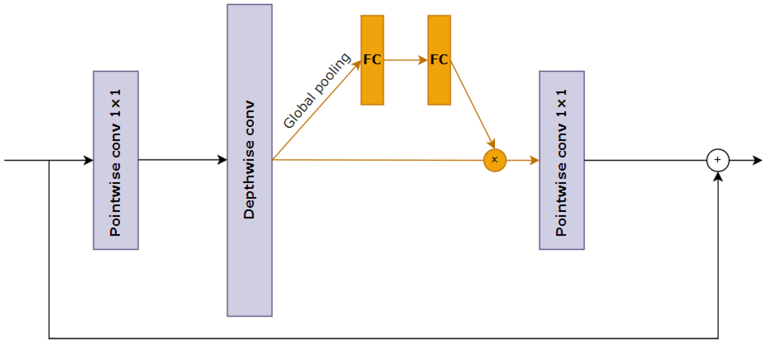
25]—the mobile inverted bottleneck convolution (MBConv). The structure of the building block is illustrated in
Figure 4. It consists of a depthwise separable convolution used in an inverse bottleneck structure and, in many cases, a squeeze-and-excitation unit.
While it has been shown to be a computationally efficient building block, recent work has shown that the large variation within layers of edge models due to the use of various diverse compression techniques results in throughput and energy efficiency shortcomings [
26].
In the remainder of this article, we evaluate alternative building blocks which differ in the convolutional layer type, the bottleneck structure and the inclusion of a squeeze-and-excitation unit.
4.2. Setup
We evaluate building blocks for mobile vision models based on the
RegNet design space [
20]. This is defined by four parameters: depth
d, initial width
, slope
and quantization
. Instead of making the width of every block in the neural network a hyperparameter, the RegNet design space parameterizes the block widths as
for
. This block width is additionally quantized through the hyperparameter
, such that the network only increases width at each of the four stages, where each stage consists of a sequence of identical blocks (see [
20] for more details).
For all evaluations, we sampled 130 models (as described in
Section 3.2) from the design spaces created by the evaluated building block and trained each model for 10 epochs. The models were trained using SGD and a cosine learning rate schedule with initial learning rate 0.05, a weight decay of
and a batch size of 128 on an RTX 3090.
All evaluated networks were trained on the Visual Wake Words dataset [
27]. This is specifically designed for vision models in embedded applications. It represents the vision use-case of identifying whether a person is present in an image or not. The dataset was derived from the publicly available COCO dataset and provides a realistic benchmark for tiny vision models.
4.3. Hardware Platforms
We evaluated the different mobile building block choices on a range of hardware platforms. The platforms evaluated were a CPU and GPU found in modern mobile phones, such as the Pixel 4, a dedicated hardware accelerator for edge devices (i.e., the Intel Movidius Myriad X Vision Processing Unit (VPU)), and an embedded GPU from NVIDIA found on the Jetson Nano. We also included a benchmark on a server-grade GPU to highlight the difference between choices for mobile deployment versus cloud deployment.
Table 1 gives an overview of the hardware platforms and also includes the inference framework used as it also influences the inference speed.
The latencies from the mobile CPU, mobile GPU and VPU were obtained using nn-Meter [
28], a highly accurate latency prediction library.
4.4. Depthwise Separable Convolutions versus Standard Convolutions
Since its introduction in MobileNet [
1], depthwise separable convolutions have been the de facto building block for efficient vision models. A depthwise separable convolution factorizes a standard convolution into a depthwise convolution and a
convolution called a pointwise convolution. This factorisation reduces the computations by a factor of
, where
is the number of output channels of the convolution and
K the kernel size. For the commonly used
kernel size, this means a reduction by a factor of eight to nine. While depthwise separable convolutions were initially introduced for small vision models, they became standard in vision models across all complexity ranges, for example, the very large vision model EfficientNet-L2 with 480M parameters, and 585B FLOPS also uses them.
Although standard convolutions may be more computationally expensive, they can, in certain cases, utilize the hardware resources more effectively. Hardware accelerators for DL commonly use wide single-instruction multiple-data (SIMD) processing units to achieve a high FLOP/S throughput. However high throughput can only be achieved if there is enough data re-use to fully utilize the processing units. In depthwise convolutions, the data re-use is much lower than in standard convolutions as each input feature map is only used in the computation of its corresponding output feature map. During training, resource utilization can be improved by using large batch sizes, obtaining data re-use with the convolutional kernel weights. However, during inference, where, typically, batch sizes of one are used, this places a memory bottleneck on the hardware accelerator. As a result, fused versions of the MobileNetV2 building block (Fused-MBConv), where the first pointwise and depthwise convolution are fused into a standard convolution, have recently been included in some hardware-aware neural architecture searches [
24,
29,
30] and been shown to be amongst the best models on certain hardware platforms.
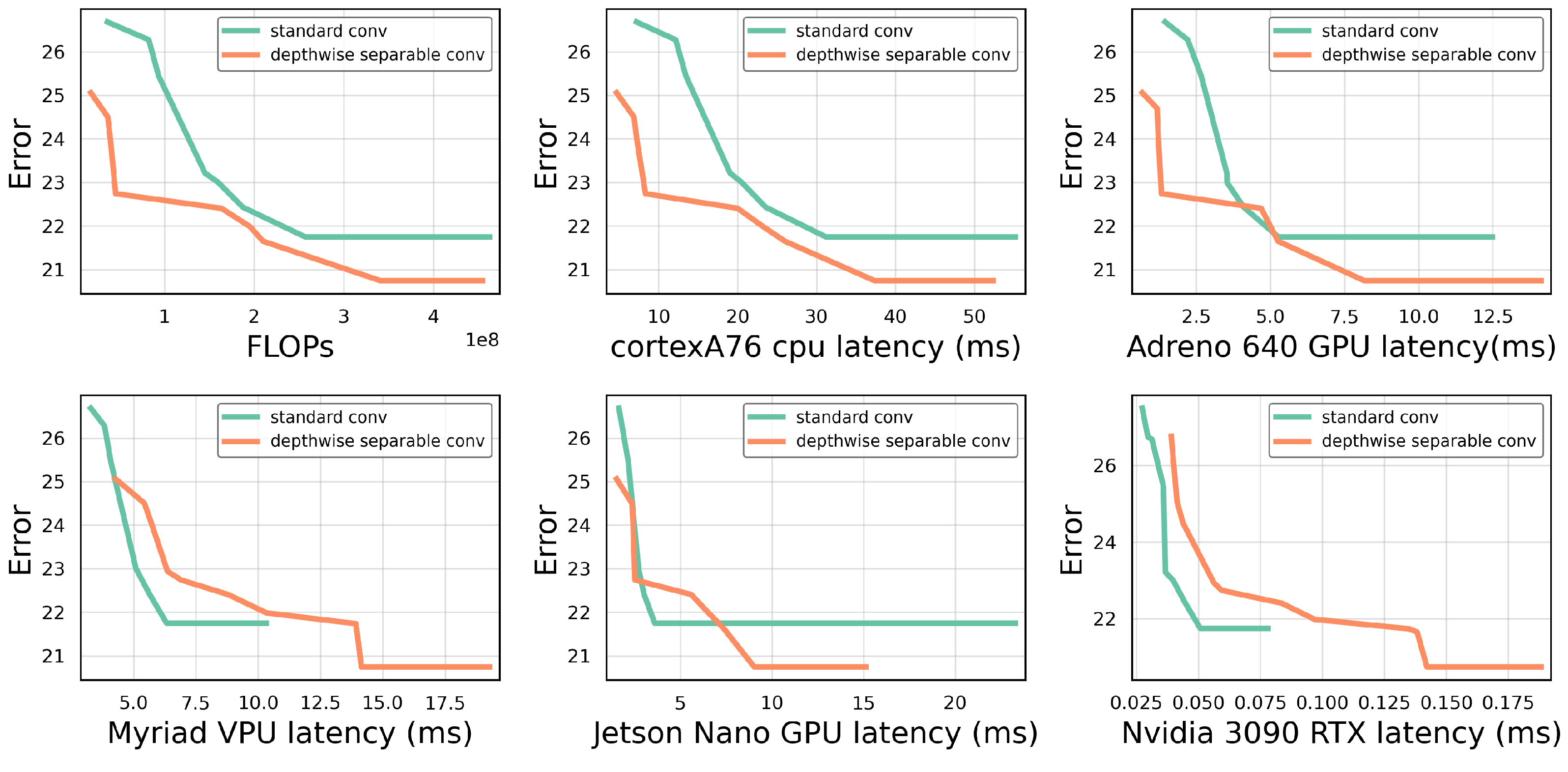
Figure 5 compares the randomly sampled pareto front of the design space based on the depthwise separable convolution to the design space based on the standard convolution. It can be seen that depthwise separable convolutions outperform standard convolutions when comparing FLOPs. The performance curves for the mobile CPU and mobile GPU have similar trend lines and also favour the depthwise separable convolutions. For the Jetson Nano embedded GPU, however, we see that the theoretical advantage of standard convolutions no longer translates into faster latency. Instead, standard convolutions outperform depthwise convolutions as the complexity grows. On the VPU and server-grade GPU, the initial order is reversed and standard convolution executes faster than the depthwise separable convolution.
To quantify the difference, we selected models with equal FLOPs from both families and compared the latencies on the different hardware platforms. On the mobile CPU, models from both families with equal FLOPs also have about equal latencies, but, on the VPU, the inference time of the depthwise separable convolution models is twice as long as for the standard convolution models. A similar trend was seen on the embedded GPU, where the latencies of those models were a factor of longer.
4.5. Grouped Convolutions
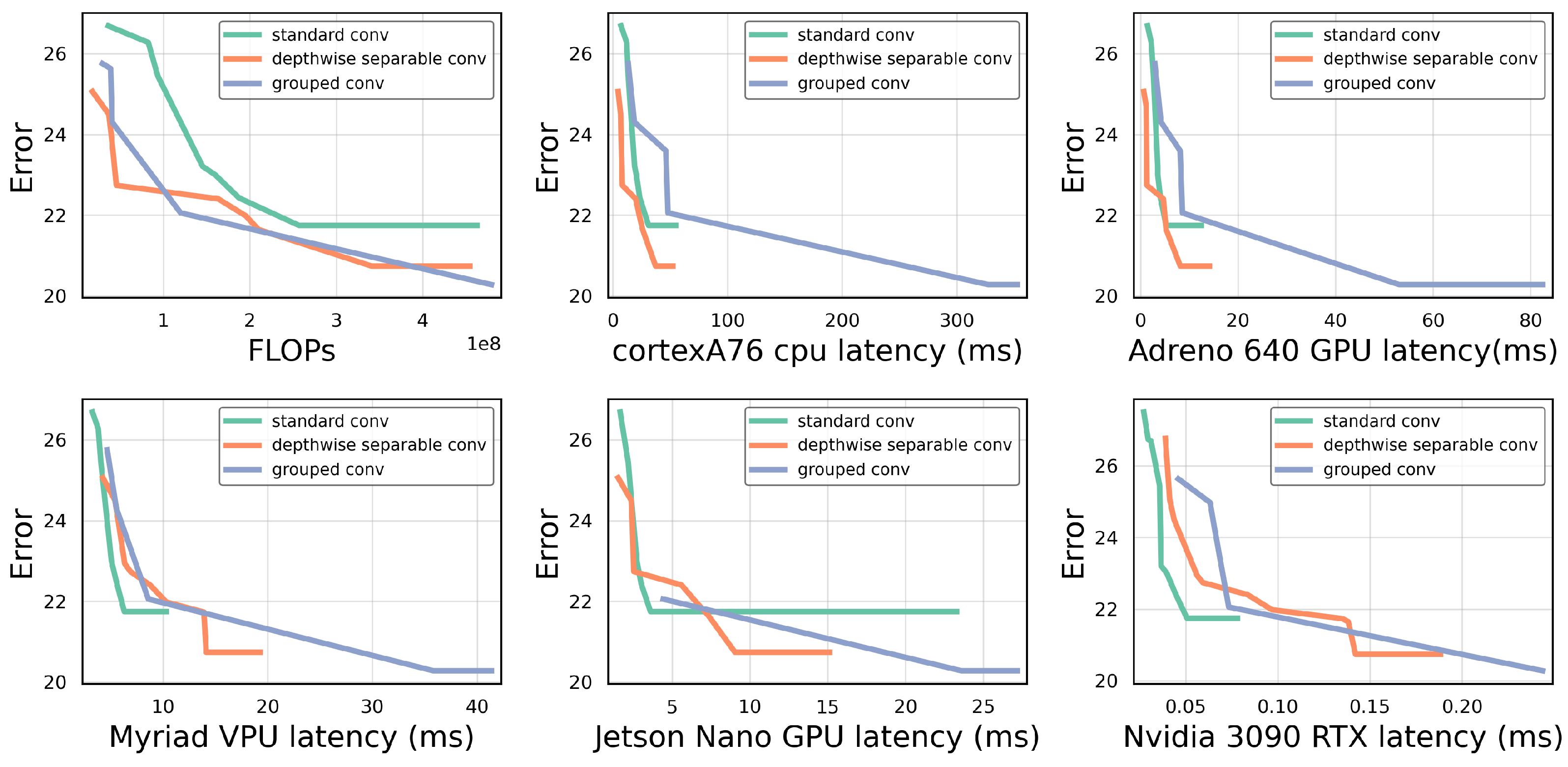
In grouped convolutions, the input channels are divided into multiple groups over which a normal convolution is performed. This puts their cost in FLOPs between those of depthwise separable and standard convolutions. This is confirmed in
Figure 6 (top left). Depthwise convolutions can be considered as a special case of grouped convolutions, where the number of groups equals the number of input and output channels. Similarly, standard convolutions are a special case where there is only one group.
In theory, grouped convolutions should be able to improve hardware utilization through their improved data reuse, while still using significantly fewer FLOPs than standard convolutions. However, current implementations in most deep learning frameworks fail to leverage these advantages, which in practice makes grouped convolutions slower than their standard convolution counterpart [
31].
Figure 6 shows that grouped convolutions are never the most promising solution on any of the tested hardware platforms. This means that, for most target latency ranges and platforms, using the much larger search space offered by grouped convolutions will rarely be beneficial. Instead, it is more efficient to narrow down the model design space to either depthwise separable convolutions or standard convolutions, based on their relative performance in trade-off plots like that shown in
Figure 6.
4.6. Bottleneck versus Inverted Bottleneck
Bottlenecks were introduced, together with residual connections, in ResNets [
8]. The main idea behind this was to lower the computational cost of each building block by performing the convolutions at a lower dimension, such that more building blocks can be stacked and deeper networks can be created without significantly increasing the computational cost.
A standard bottleneck structure consists of three convolutional layers: a
pointwise convolution to reduce the channel size, a standard convolution to improve the features, and a final
pointwise convolution to restore the channel dimensions. A parallel residual path connects the input and output of this block. In MobileNetV2 [
2], an
inverted bottleneck was introduced where the residual connection is moved to connect the bottlenecks. In practice, this means that an inverted bottleneck consists of a pointwise convolution to expand, instead of reduce, the channel dimension, a (depthwise) convolution and a final pointwise convolution to restore the original channel dimension. The motivation for this design was that it is more hardware efficient as only the bottleneck lower dimension tensors need to be fully saved to memory as the intermediate higher channel dimension tensors are only used in depthwise convolutions. This means the tensor can be split into smaller ones.
A third possibility is to use no bottleneck, since the RegNet paper found that their best models used a bottleneck expansion/reduction factor of
[
20]. When using no bottleneck, we also drop the final pointwise convolution present in bottleneck structures, since it is no longer required to make channel sizes match. All our building blocks in this comparison make use of depthwise convolutions.
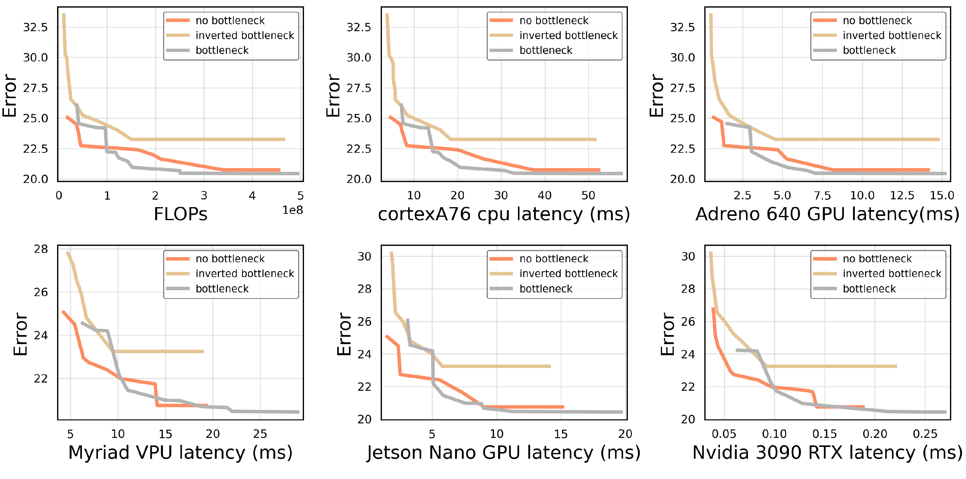
The results, as shown in
Figure 7, indicate that using inverted bottlenecks degrades performance and fails to deliver the promised expected inference speedup. In general, across all hardware platforms, the blocks without a bottleneck and with a regular bottleneck show very similar performance. It can be observed that the VPU and server-grade GPU slightly favour the building block without a bottleneck as it executes faster compared to bottleneck blocks. These are the same hardware platforms as those where the standard convolution outperformed the depthwise separable convolution, indicating that pointwise convolutions underperform on these platforms.
4.7. Squeeze-and-Excitation Unit
A squeeze-and-excitation (SE) [
4] block is an architectural unit for convolutional neural networks that performs dynamic channel-wise feature recalibration to improve the representation power of a convolutional building block. Given input
, the SE unit first squeezes the spatial information using global average pooling:
This step is followed by an excitation step that recalibrates the channels:
where
and
are two learned linear transformations and
refers to the sigmoid activation function. The final output
of the SE unit is obtained by scaling the original inputs
:
, where · refers to the channel-wise multiplication.
MnasNet [
15] brought the SE unit to mobile vision networks, as they were shown to improve model performance compared to previous state-of-the-art models with similar latency. More recently, however, squeeze-and-excitation modules have been removed from mobile vision architectures when they are deployed on embedded ML accelerators. EfficientNet-lite [
32] and MobileNetEdgeTPUv2 [
33], for example, remove the SE unit as they claim it is not well supported for mobile accelerators, such as the Google EdgeTPU.
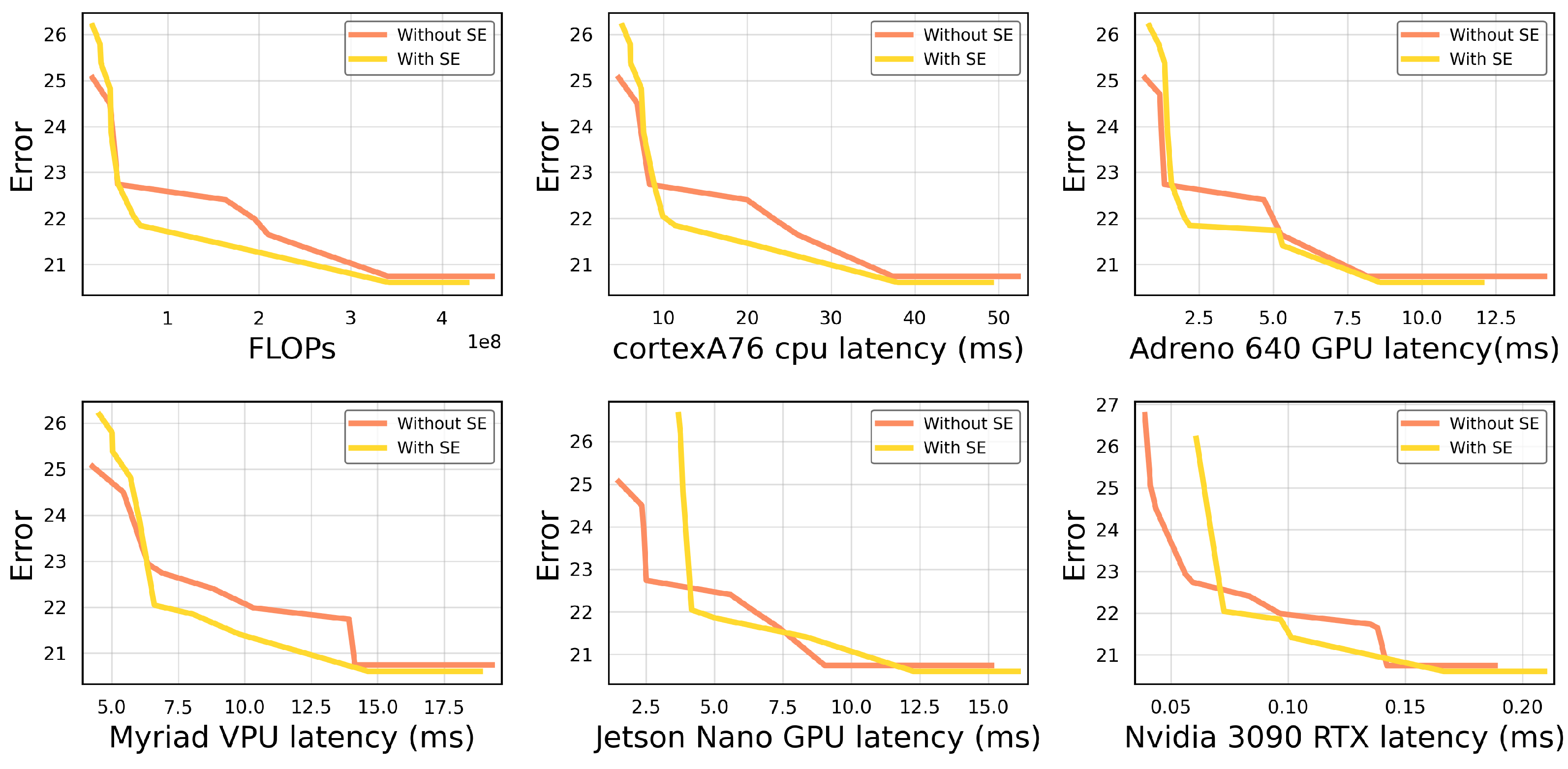
We evaluated the SE block by comparing design spaces with the depthwise separable building block, with and without an SE unit extension.
Figure 8 shows that the SE block is a favorable addition for certain mobile platforms as it is very FLOPS-efficient. This translates to it being more optimal for mobile CPUs and GPUs. However, for the embedded Jetson Nano GPU, it is no longer a clear benefit to include the SE unit as it fails to exploit the optimizations for convolutional kernels and adds a significant delay. Comparing models with and without the SE unit and with equal execution time on a mobile CPU, we found that those same models without the SE unit have a running time that is up to a factor of
longer on the embedded Jetson Nano GPU.
5. Conclusions
Developing a new model for a targeted hardware platform, and with given design constraints, requires careful consideration of the building block. An evaluation based on FLOPs often leads to misleading conclusions with respect to the relative benefits of the components in the standard MBConv block on specific hardware platforms. We developed a methodology that can be used to select building blocks and constrain the design spaces as a first step in the network design process (i.e., as a preselection step before NAS) in a hardware-aware manner, while maintaining the freedom to trade-off between task performance and execution efficiency.
We used our approach to evaluate the hardware efficiency of different convolutional building blocks on various hardware platforms. Our results show that execution of building blocks with components that are theoretically efficient, such as the SE unit, take a factor of longer to execute than their non-optimized counterparts due to better hardware utilization on platforms with specific embedded ML accelerators, such as the Intel NCS2 or the Nvidia Jetson Nano.
In essence, the insights gained from this investigation highlight the importance of benchmarking the building blocks used in mobile vision neural networks, which has been overlooked in the past. We believe that our methodology will be key to the development of hardware-aware neural networks for deployment on edge devices.

