Article

Seismic Imaging of Complex Velocity Structures by 2D Pseudo-Viscoelastic Time-Domain Full-Waveform Inversion

by
Niloofar Alaei
1,
Mehrdad Soleimani Monfared
1,2,*,
Amin Roshandel Kahoo
1 and
Thomas Bohlen
2
1
Department of Mining Petroleum and Geophysics Engineering, Shahrood University of Technology, Shahrood 3619995161, Iran
2
Geophysical Institute (GPI), Karlsruhe Institute of Technology (KIT), 76131 Karlsruhe, Germany
*
Author to whom correspondence should be addressed.
Appl. Sci. 2022, 12(15), 7741; https://doi.org/10.3390/app12157741
Submission received: 27 June 2022 / Revised: 29 July 2022 / Accepted: 30 July 2022 / Published: 1 August 2022
(This article belongs to the Special Issue Advancing Complexity Research in Earth Sciences and Geography)

Abstract

:
In the presented study, multi-parameter inversion in the presence of attenuation is used for the reconstruction of the P- and the S- wave velocities and the density models of a synthetic shallow subsurface structure that contains a dipping high-velocity layer near the surface with varying thicknesses. The problem of high-velocity layers also complicates selection of an appropriate initial velocity model. The forward problem is solved with the finite difference, and the inverse problem is solved with the preconditioned conjugate gradient. We used also the adjoint wavefield approach for computing the gradient of the misfit function without explicitly build the sensitivity matrix. The proposed method is capable of either minimizing the least-squares norm of the data misfit or use the Born approximation for estimating partial derivative wavefields. It depends on which characteristics of the recorded data—such as amplitude, phase, logarithm of the complex-valued data, envelope in the misfit, or the linearization procedure of the inverse problem—are used. It showed that by a pseudo-viscoelastic time-domain full-waveform inversion, structures below the high-velocity layer can be imaged. However, by inverting attenuation of P- and S- waves simultaneously with the velocities and mass density, better results would be obtained.

1. Introduction

Imaging of geological complex structures in the subsurface can be used for geotechnical site characterization by geophysical methods. The term ‘complex’ is used for those subsurface earth models which cannot be easily imaged by conventional seismic imaging methods due to their complex velocity structures or geometry. Examples of complex structures can be steep dipping beds, intensive faulted or folded media, and earth models with strong velocity changes. In addition, the near-surface velocity anomalies can increase complexity of imaging problems, mostly due to the complexity in the simulation of the seismic wave propagation, or in other words, the complication caused by the propagation of the body waves through the complex near-surface layers [1]. The most realistic of such situations is the near-surface salt layers which can or cannot play a role as the caprock for petroleum reservoirs. In those cases, the fluids trapped in the layers beneath the salt have considerable effects on the elastic properties of the subsurface media. The better these properties are modeled, the more accurate an image of the subsurface will be obtained.
Conventional seismic imaging methods are no more reliable in solving imaging problems raised from complex geological media. High quality seismic imaging is needed in most exploration studies such as gas storage projects, geological hazard, CO2 storage projects in target finding and monitoring, and also in geothermal resources. To obtain a high-quality seismic image, further investigation of obstacles to obtaining reasonable seismic images and developing reliable imaging methods are required. Considering the problems of seismic imaging in complex media, it was stated that poor seismic images from different regions mostly resulted from the application of inappropriate imaging algorithms [2]. The minor concerns were related to the data acquisition problems due to harsh topography, but the major issues are rooted in extreme complexity in subsurface media and poor quality in signal to noise ratio (SNR) [3]. The former could be resolved by adequate acquisition; however, the later requires deep investigation on developing proper imaging tools. In one study, it was proposed resolving obstacle partially by the common reflection surface (CRS) and the normal incidence point (NIP) tomography method [4]. However, the CRS still suffers in handling strong lateral velocity changes or geologically complicated media [5]. The reverse time migration (RTM) and the full waveform inversion (FWI) methods, as the latest introduced methods, deal with a vast majority of problems in seismic imaging [6,7]. However, these methods are still present issues in application to large field datasets, poor quality data with shortage in frequency content, and low SNR in the low frequency part of the data [8]. Challenges for FWI land applications consist of addressing the wavefield propagation from rough topography, low SNR of the low-frequency data, and determination of an appropriate source wavelet throughout the iterations by improving the velocities and model parameters [9].
The FWI employs an iterative procedure that is based on a forward modeling and inversion procedure to find the optimal parameters [10,11]. Some studies have been carried out to show the efficiency of FWI in the imaging of complex media [7], presented the application of the FWI method in the frequency domain on the wide-aperture onshore seismic data with a complex geological setting (thrust belt) [12], and applied the elastic frequency-domain FWI to the synthetic onshore Marmousi2 model [13]. They implemented a velocity-gradient starting model and a very low starting frequency to image the complex structure model. Reference [14] also tested the application of this strategy to the offshore versions of the synthetic Marmousi2 model. They successfully imaged the complex model using their strategy. Reference [8] presented a parallel 2D elastic frequency-domain FWI algorithm based on a discontinuous forward problem [15] that was applied to a realistic synthetic onshore case study. They obtained a high-resolution P- and S- wave velocity of the complex onshore structure using a joint inversion of the surface and body waves recorded by a wide aperture acquisition geometry. Reference [16] studied the application of the FWI method in the time-domain on the problem of subsalt imaging with the modified Flooding Technique and showed the difference between the results of elastic and acoustic FWI methods. These differences reveal that the result of the acoustic FWI algorithm on elastic data for the subsalt imaging problem is not reliable. The application of the multi-parameter viscoelastic FWI using a frequency-domain on synthetic data example was proved by [17]. The low-order finite element discontinuous Galerkin method was used to solve the forward problem which can be a good option when studying the complex topographies and high-velocity contrasts, and the quasi-Newton L-BFGS optimization was implemented to estimate the inverse of the Hessian matrix in order to decrease the computational cost and improve the reconstruction of the velocities, density, and attenuation parameters. Reference [9] implemented the FWI-SIMAT algorithm to investigate the capability of the acoustic FWI in the reconstruction of the Marmousi velocity model both in the time and frequency domain. Reference [18] used a developed FWI method in which a two-stage sequential approach (SFWI) was tested on the field datasets recorded in the Black Sea and in the shallow-water area of a river delta in the Atlantic Ocean to obtain detailed subsurface images containing rock formations that might be potential gas deposits. Most applications of the FWI methods on complex structures have been performed in the frequency domain or ignored seismic wave attenuation. Ignoring the viscous effect of the propagation media provides an unrealistic reconstructed S- wave velocity model, especially in the study of the complex geologic media [19]. Reference [20] showed that taking key elements properly into account, FWI produces a reliable high-resolution near-surface model that could not be otherwise recovered through traditional methods. Although few attempts have been reported that incorporate FWI for land studies [18]; however, they were convincing in providing acceptable seismic image. Therefore, it is supposed that deriving a processing workflow modified for accurate imaging of seismic data from complex regions would be promising in resolving the problem of low SNR and strong lateral velocity changes due to complexity in wave propagation media.

2. Problem Statement

It was shown that seismic imaging in seismic data with above mentioned properties is technically a challenging task due to several reasons. The first is complexity of the media. These complexities will introduce lateral velocity changes, make reduction in quality of data and reduce SNR of data. These problems prevent application of conventional imaging methods and require advanced methods, such as RTM and FWI, to be modified accordingly. The FWI method estimates subsurface properties affecting the seismic wave-field via minimizing the field data and synthetic seismogram generated from forward modeling. An ultimate FWI method should take attenuation and dispersions into account, which means considering the wave propagation medium as a viscoelastic medium. An appropriate choice of model parameterization is also very important in viscoelastic FWI. Various approaches are presented for FWI in viscous media in the frequency and time domain [21]. Shot parallelization, variable grids in the near future and better free surface implementation are also other compatibilities of an appropriate FWI method. Obviously, to make the inversion process converge to the correct and accurate response, the initial velocity model needs to be close enough to the real field velocity model. The focal issue here is to resolve the problem of imaging on data which contains a high-velocity layer and causes less energy of transmitted wavefield reach to the structures under this layer. Presence of steep dips, low SNR, and energy absorption by thick layers of evaporites—which dramatically reduce the quality of images in deeper parts—are obstacles in obtaining high quality images. Since the data suffer from reduction in quality due also to faults and variations in the thickness of the high-velocity layer, it is required that the FWI method modified accordingly in considering attenuation and wavelet estimations [22]. The lateral velocity changes due to the evaporites will reduce the sensitivity of the FWI method in reconstruction of the velocity models. Therefore, it is important to define appropriate initial velocity models. Furthermore, since the FWI package of the Karlsruhe institute of technology (KIT) could model the viscoelastic properties of the media in wave propagation simulation, it is assumed that the data quality will increase in regions with above mentioned problem [23]. The model parameterization and discretization of the media is also challenging in application of FWI method in such regions. Discretization should be flexible and appropriate for boundaries of abrupt changes in elastic properties of the media, which is the result of complex mud intrusions [24]. This complexity will also introduce problems in model parameterization, which needs to be optimized via parameter analysis. In this study, the performance of the 2D pseudo-viscoelastic FWI proposed by [20] to image a synthetic model with velocity complexity is investigated. A time-domain multi-parameter FWI is applied to reconstruct the P- wave velocity, S- wave velocity, and density models. The forward problem is solved using the finite difference method (FD) and the viscoelastic wave equation is discretized considering the convolutional perfectly matched layers (PMLs) absorbing boundary condition to prevent the edge effects. To solve the inverse problem, the preconditioned conjugate gradient (PCG) is used. The gradients are computed with the adjoint-state method. A simple model generated by the 1D linear gradient is considered as the initial model.

3. Theory

3.1. Forward problem

In this study, the stress–velocity equation of the wave equation in the time domain in an anisotropic viscoelastic medium with rheology described by a GSLS [25,26] is taken to solve the forward problem [27,28]:
ρ ν i t = σ i j x j + f i
σ ˙ i j = ν k x k { M ( 1 + τ p ) 2 μ ( 1 + τ s ) } + 2 ν i x j μ ( 1 + τ s ) + l = 1 L r i j l i f i = j ,
σ ˙ i j = ( ν i x j + ν j x i ) μ ( 1 + τ s ) + l = 1 L r i j l i f i j
r ˙ i j l = 1 τ σ l { ( M τ p 2 μ τ s ) ν k x k + 2 ν i x j μ τ s + r i j l } i f i = j ,
r ˙ i j l = 1 τ σ l { ( M τ s [ ν i x j + ν j x i ] + r i j l } i f i j .
where σ i j denotes the i jth component of the stress tensor, ν i denotes the components of particle velocity, f i is the components of external body force, ρ is density, M is the P- wave modulus, and μ is the S- wave modulus. r i j l denotes the L memory variables ( l = 1 , , L ) which correspond to the stress tensor σ i j , τ σ l , are the L stress relaxation times for P- and S- waves and τ p , τ s are the level of attenuation for P- and S- waves respectively. It is necessary to mention that the dot over symbols indicates partial differentiation with respect to time. The attenuation of rocks is defined by the seismic quality factor (Q):
Q ( ω , τ σ l , τ ) = 1 + l = 1 L ω 2 τ σ l 2 1 + ω 2 τ σ l 2 τ l = 1 L ω τ σ l 1 + ω 2 τ σ l 2 τ
where   ω   is the angular frequency, and the variable τ denotes
τ = τ ε l τ σ l
where τ σ l is the stress relaxation time, and τ ε l is the strain retardation time for the lth Maxwell body of the GSLS. With Equation (6), L + 1 parameters τ σ l , τ are obtained that describe a constant Q-spectrum within a limited frequency range by a limited number of Maxwell bodies [27]. The forward problem is solved by using a time-domain two-dimensional second order FD operator in time and space on a staggered grid [27]. To reduce the edge effects and reflections at the boundaries the CPMLs are implemented [29,30].

3.2. Inverse Problem

FWI is a non-linear optimization problem that needs an appropriate objective function to be minimized. The L2-norm of the data residuals as the objective function E is used in the presented study [28,31].
E = s = 1 n s r = 1 n r j = 1 n c 0 T ( d j ( x s , x r , t ) , s j ( x s , x r , t , m ) ) 2   d t
where d j denotes the observed data, and s j is the synthetic data at receiver r at point x r . n s and n r are the number of sources and receivers respectively. n c is the number of components and T is the recording time. The PCG method [32] is implemented to minimize the objective function by iteratively updating the model parameters m along the conjugate direction δ c n
δ c n = δ m n + β n δ c n 1
At the first iteration step ( n = 1 ), the model is updated along the steepest descent direction
m 2 = m 1 + μ 1 δ m 1
The model is updated along the conjugate direction in all subsequent steps ( n > 1 )
m n + 1 = m n + μ n δ c n
where δ c 1 = δ m 1 .   μ n denotes the step length that is estimated by a parabolic line search method [33,34,35,36]. The weighting factor beta is calculated using the Polak–Ribiere formulation:
β n P R = δ m n T ( δ m n δ m n 1 ) δ m n 1 T δ m n 1
δ m n = E m denotes the gradients of material parameters that can be calculated using the adjoint state method [28,32,37,38]. The model parameters can be density ρ and unrelaxed P- and S-wave moduli π u , μ u for a viscoelastic medium assuming a constant a priori known quality factor Q . The gradients of the misfit function for the unrelaxed moduli of a grid cell at a point x can be calculated by a zero-lag cross-correlation of the forward propagated s and the adjoint wavefield s are approximated [28].
E π k = 0 T ( s 1 ( x " , T t ) x 1 + s 2 ( x , T t ) x 2 ) . ( s 0 1 ( x , t ) x 1 + s 0 2 ( x , t ) x 2 ) d t Δ x 3
E π μ k = 0 T [ ( s 1 ( x " , T t ) x 2 " + s 2 ( x " , T t ) x 1 " ) . ( s 0 1 ( x " , t ) x 2 " + s 0 2 ( x " , t ) x 1 " ) + 2 ( s 1 ( x " , T t ) x 1 " s 0 2 ( x " , t ) x 2 " + s 2 ( x " , T t ) x 2 " s 0 1 ( x " , t ) x 1 " ) ] d t Δ x " 3
E ρ k = 0 T ( s 1 ( x , T t ) t s 0 1 ( x , t ) t + s 2 ( x , T t ) t s 0 2 ( x , t ) t ) d t Δ x 3
The parametrization considered in this study is ( ρ , V p , V s ). The gradients are calculated for these parameters using the chain rule. To change the parametrization from the parameters ( ρ , π u , μ u ) to ( ρ , V p , V s ) one can apply the chain rule according to the relations of unrelaxed moduli with the unrelaxed Lamé parameters ( ρ , λ u , μ u ) and seismic velocity parameters respectively (Equations (16) and (20)).
ρ = ρ , π u = λ u + 2 μ u ,   and   μ u = μ u
The gradients for density and Lamé parameters can be expressed by
E ρ = E ρ ρ ρ + E π u π u ρ + E μ u μ u ρ = E ρ
E λ u = E π u π u λ u + E μ u μ u λ u + E ρ ρ λ u = E π u
E μ u ' = E π u π u μ u ' + E μ u μ u μ u ' + E ρ ρ μ u ' = 2 E π u + E μ u = 0 T [ ( s 1 x 2 + s 2 x 1 ) . ( s 0 1 x 2 + s 0 2 x 1 ) + 2 ( s 1 x 1 s 0 1 x 1 + s 2 x 2 s 0 2 x 2 ) ] d t Δ x 3
with the relations
ρ = ρ   a n d   v p = λ + 2 μ ρ λ = ρ ( v p 2 2 v s 2 )
v s = μ ρ μ = ρ v s 2
one obtains
E v p = 2 ρ v p E λ
E v s = 4 ρ v s E λ + 2 ρ v s E μ
E ρ = ( v p 2 2 v s 2 ) E λ + v s 2 E μ + E ρ
It is worth noting that an approximated Hessian (after [39]) is applied as an appropriate preconditioning operator P to the gradient δ m before updating the model parameters. The Hessian is calculated for each shot individually and will be applied to the gradient from each shot directly. A multi-scale inversion strategy is implemented to reduce the high nonlinearity at the beginning of the inversion and pass the cycle skipping problem [40].

4. Synthetic Data Example

In this section, a synthetic example is performed to investigate the capability of 2D pseudo-viscoelastic FWI in the time domain to image shallow complex structures using IFOS2D. The true model used to simulate the observed data for three parameters (P- wave and S- wave velocity model and density model) is generated inspired by a real model located in Iran, which contains large synclinal shape of evaporite layers with very high velocity, faulted in the left side and the thickness of the high-velocity layers varies through the section. The seismic velocity of this evaporite layers is between 3840 and 5420 m/s, according to the percent of the containing salt compare to anhydrite, depth and thickness of the layer, which is in the range investigated in different studies [41,42]. The surrounding carbonate and shale layers show velocities around 2800–3420 m/s. The main problem in the seismic data with the abovementioned problem is to image target layers below the high-velocity layer, which is supposed to be resolved by FWI method. Therefore, in our study, in the first step, we tried to build a synthetic model with same geometry and shape of the high-velocity layer. In the next step, we tried to select velocities for each layer according to the real velocity of the media. In this step, since the provided forward and reverse codes for FWI in this study are mainly used for near-surface data, rather than deep seismic; so to prevent instability in analysis, we scaled down all the velocities of the layers in the model with a constant value. Therefore, we modeled the high-velocity layer near the surface with velocity close to 600 m/s. It should not be considered as the real high-velocity layers in deep earth, but a downscaled version of that.
Due to high velocity, propagation of the surface and body waves through the complex near-surface layers would be more complicated. This example can test the capability of the FWI to image a complex velocity structure. The model space has a size of 400 grid points in the horizontal direction and 160 grid points in the vertical direction. Therefore, the actual dimension would be 50 × 20 m considering a grid spacing of 0.125 m. A total of 19 shots and a total of 73 receivers located at the constant depth of 0.2 m that record both horizontal and vertical components are used. A cubed sine wavelet with a center frequency of 31.25 Hz generated by a hammer source is used as the source signal. The CPML frame is marked by the black dashed line. A viscoelastic medium is considered in this example and approximated a constant quality factor of Q s = Q p = 20 in the analyzed frequency band up to 60 Hz (a high-cut frequency filter of 10, 20, 30, 40, 50, and 60 Hz is used in stages) with three relaxation mechanisms of a generalized standard linear solid. A minimum of five iterations are taken into account at each stage. A 1D linear gradient is used to build the background of the true model and the background is considered as the initial model for each parameter in inversion. All models are updated simultaneously during inversion. It is worth mentioning that the true and initial velocity models are built with a v p v s ratio of 1.5 and a total propagation time of 0.6 s is considered. Initially, we tried the Vp/Vs ratio of 1.5 because it is the minimum ratio which can be used as a reasonable value for sediments or soft rocks near the surface. In the following, we have selected the Vp/Vs ratio of 2.5 which is more realistic for our example. The PCG is carried out to solve the inverse problem.

5. Results

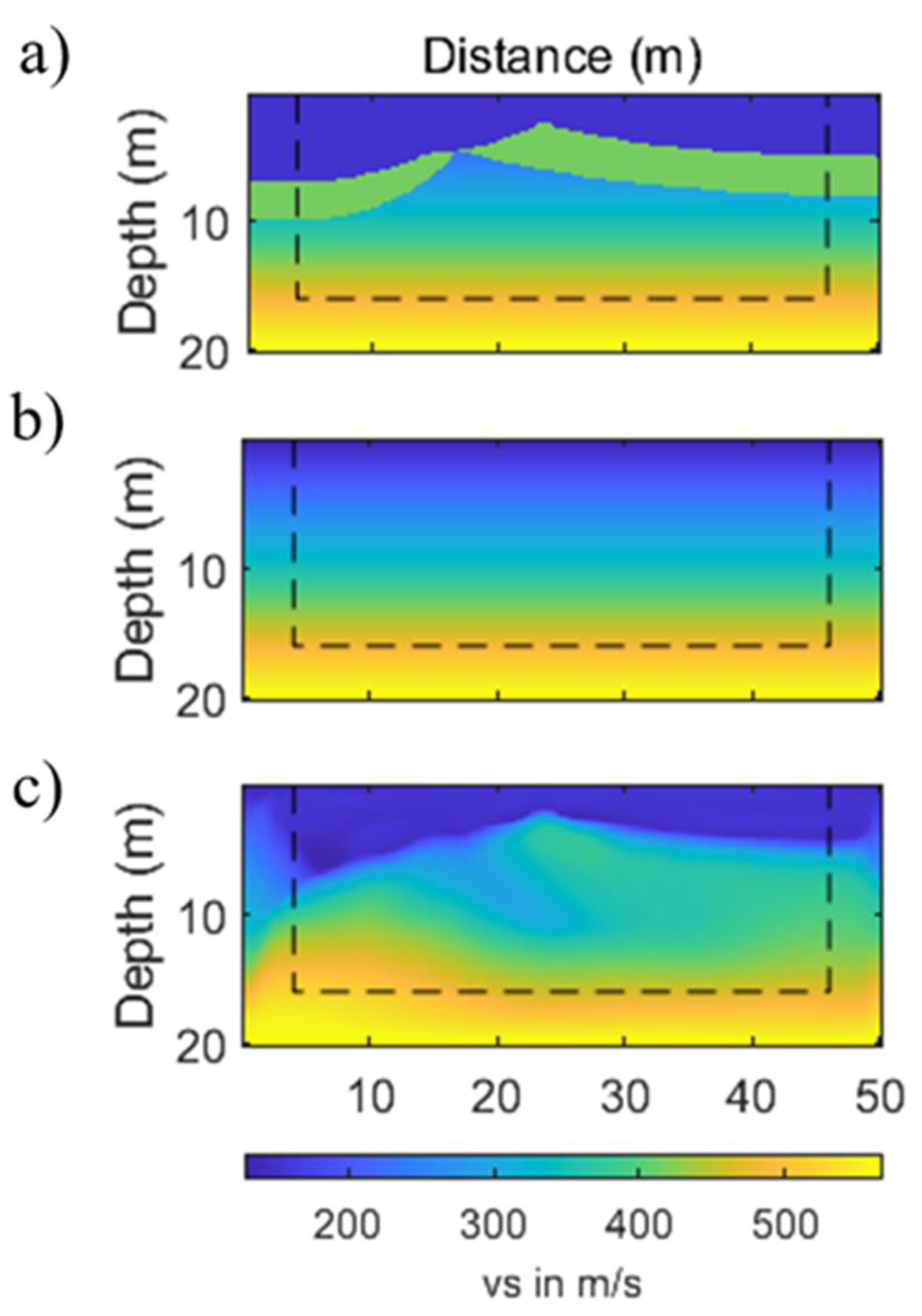
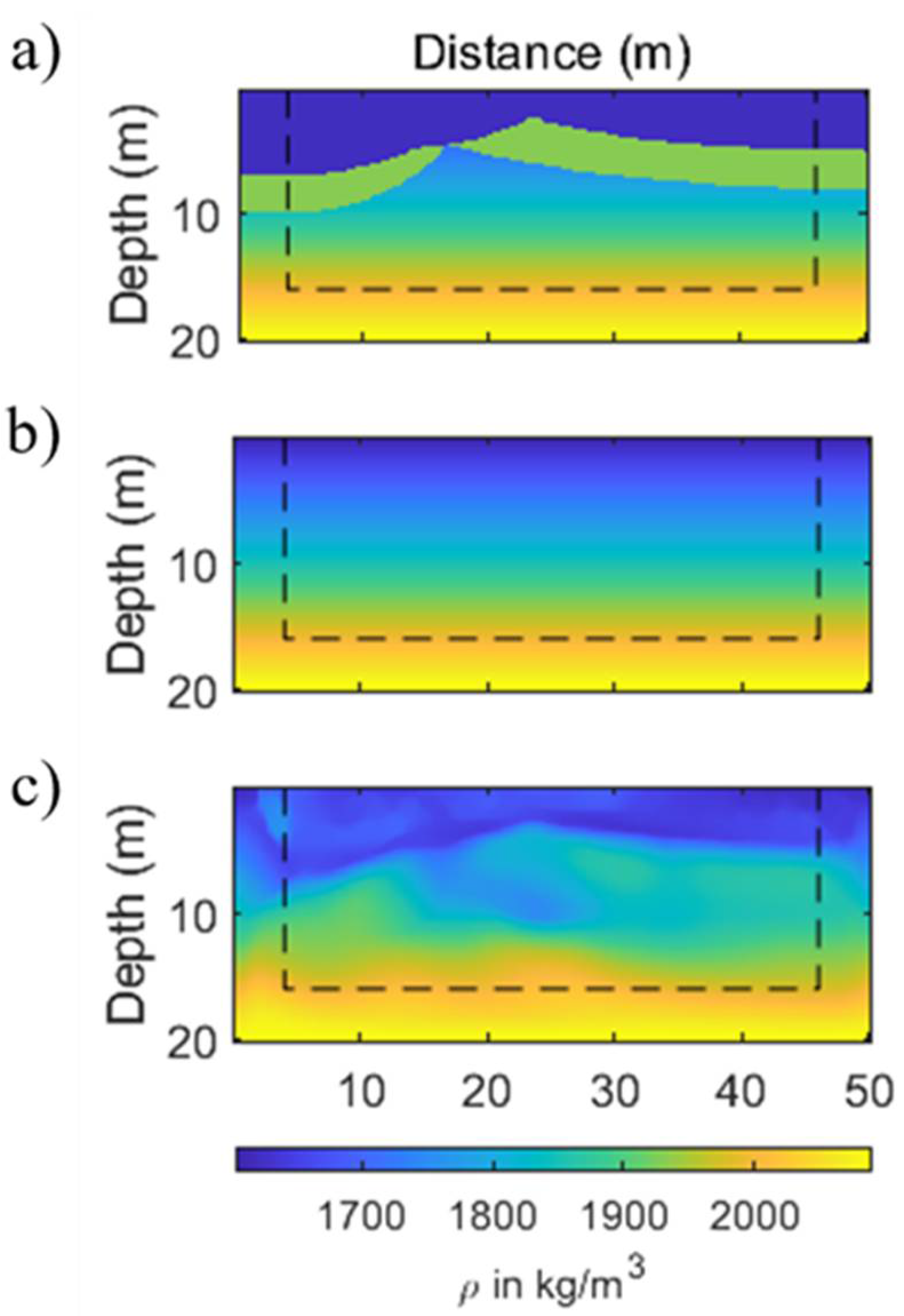
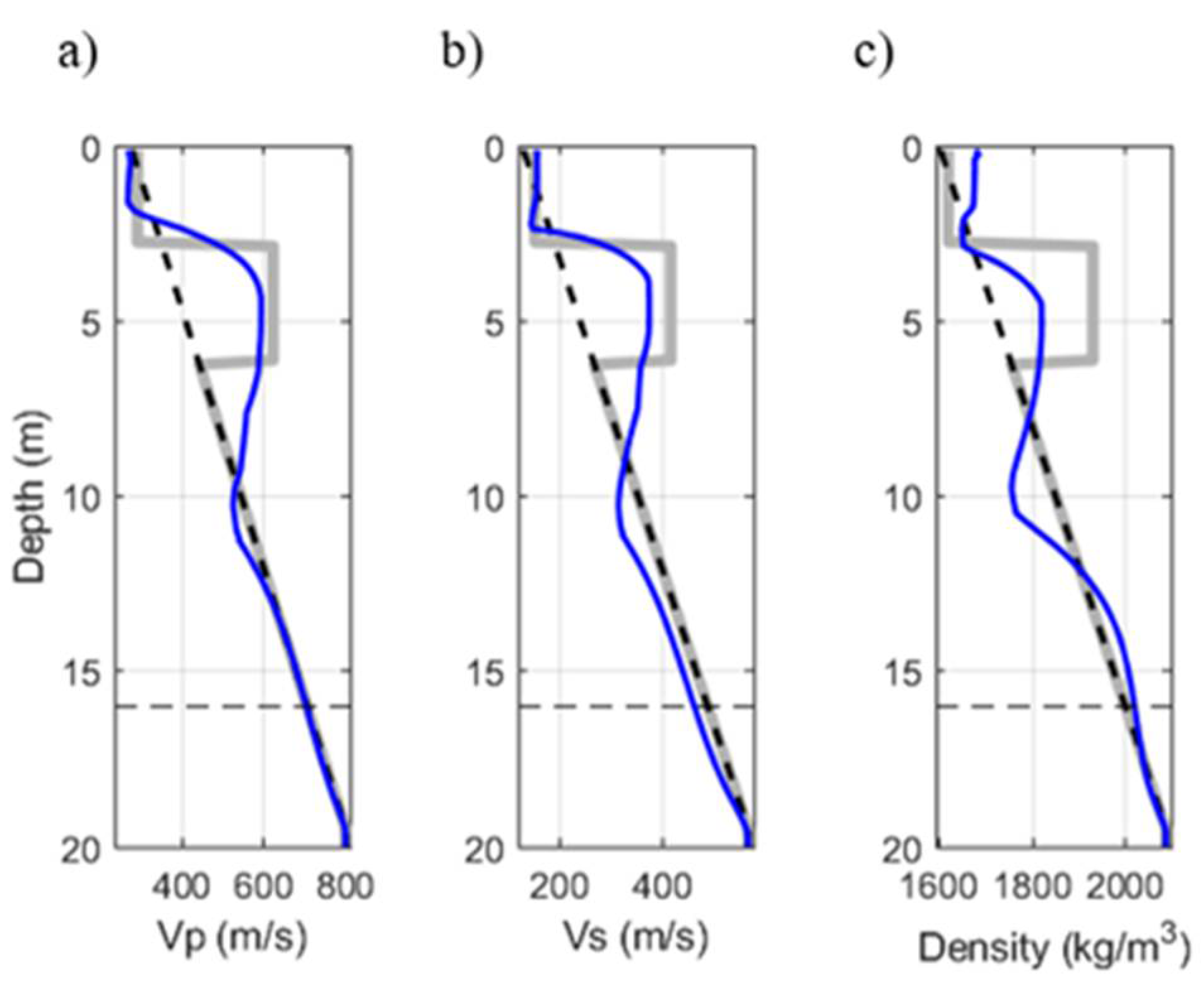
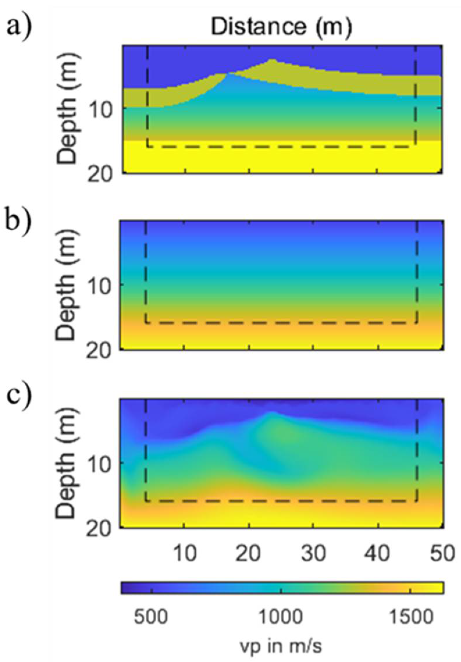
In this study, 314 iteration steps are calculated, and the inversion takes about 10 h when using a system with four cores with 3.1 GHz speed and 16 Gb of ram. The true, initial, and inverted P- wave velocity models are shown in Figure 1. The same order is given, for the S- wave velocity and density models in Figure 2 and Figure 3, respectively. Figure 4 shows the vertical profiles through the P- wave and S- wave velocity and density models that are considered to compare the results with the true model in more detail. Vertical profiles through the models are obtained at x = 25   m . The reconstructed models are in good accordance with the true models, especially for the S- wave velocity model. In the inverted S- wave velocity model, the upper edge of the high-velocity layer can be seen more sharply compared to the two other models. The bottom edge of the high-velocity layer is reconstructed in each model but not in the accurate location. Some artifacts are seen in the low-velocity zone of the density and P- wave velocity models. Regarding the low sensitivity of surface waves with respect to the P- wave velocity and density model [41], inaccurate results of inversion for the P- wave velocity and density models can be expected, also because the amplitude of surface waves is much higher than the amplitude of P- waves. The sensitivity of surface waves with respect to the P- waves is low and it leads to an inaccurate P- wave velocity model at each iteration step.
Because the density model is in relation to the P- wave velocity model using an empirical relation. Therefore, it affects the density model and the result of these two models is not as accurate as of the inverted S- wave velocity model [42].
To assess the results precisely, the final synthetic shot gathers are compared with the observed data. The vertical velocity seismogram of the shot at x = 9 m is obtained and the seismograms for the initial models are calculated for trace 36 of the shot and compared with the seismogram of the observed and inverted model. The comparison of the synthetic and observed seismograms of the shot at x = 9 m is shown in Figure 5a and the comparison of the initial, observed, and inverted data for trace 36 at this shot is shown in Figure 5b. Each seismogram is normalized to its maximum amplitude. The comparison of the initial and inverted data indicates the good performance of the inversion method and application of the software IFOS2D (Inversion of Full Observed Seismograms (2D)) in reconstructing model parameters. The calculated data agreeably fit the observed data. Therefore, the inversion result is a model which better explains the observed data. In the following, the true and initial models are built considering the v p v s ratio of 2.5 that is more realistic in the case of studying the soft rocks near the surface. In this case, due to the increase in the velocity values, the wavelengths propagated through the medium are increased and the resolution is influenced by the wavelength. The high-velocity layer is not resolved with the P- wave velocity model. Therefore, to reconstruct the model, a broad bandwidth of the source signal is needed. A broad bandwidth signal cannot be generated by a hammer source, thus a vibroseis source can be used to generate a signal which has a higher center frequency and covers a broader frequency range than a cubed sine wavelet [43,44]. Since a Ricker wavelet is similar to a Klauder wavelet generated by vibroseis source and is used in the synthetic seismic modeling, in the following a Ricker wavelet with a center frequency of 50 Hz is considered as the source signal.
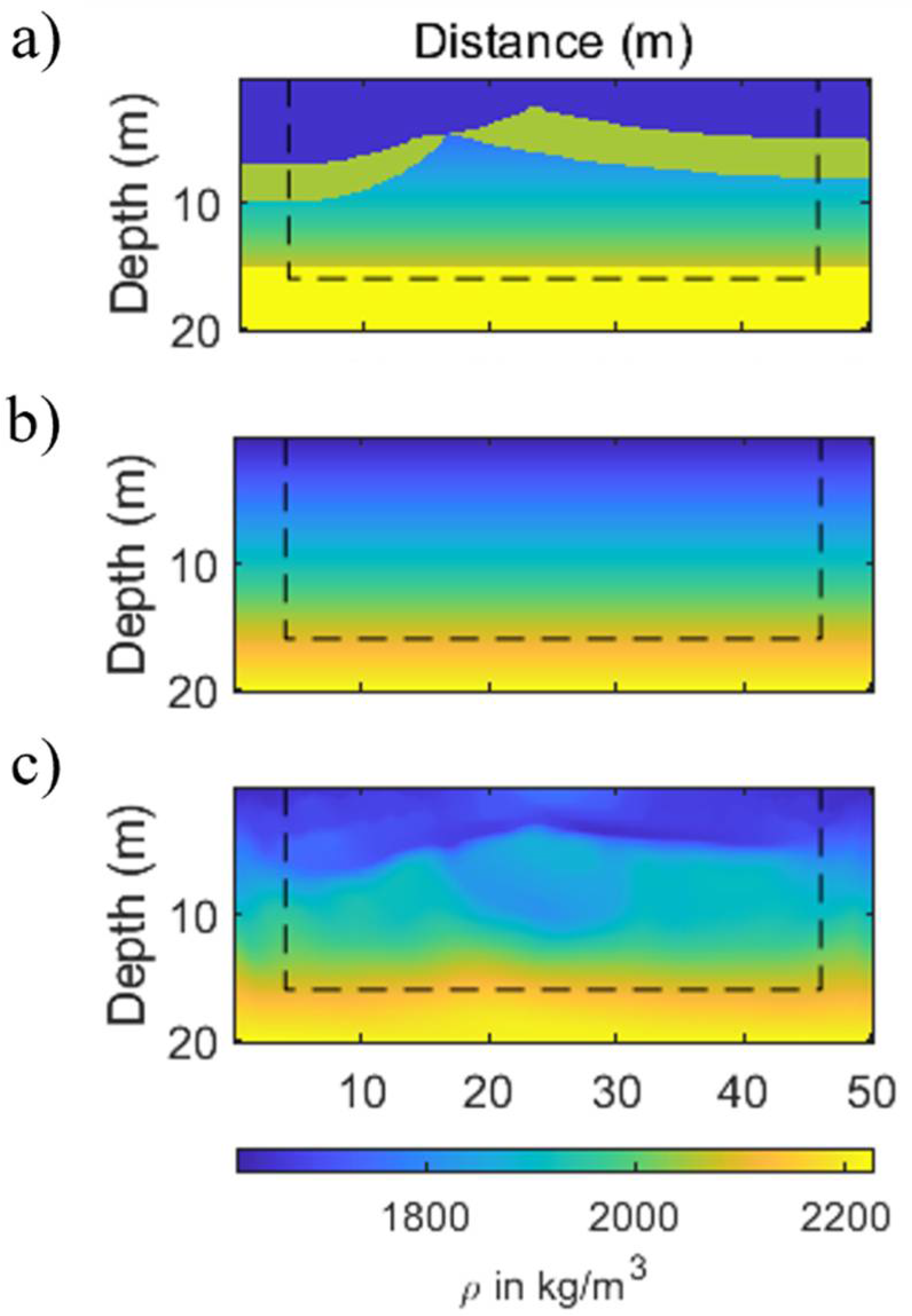
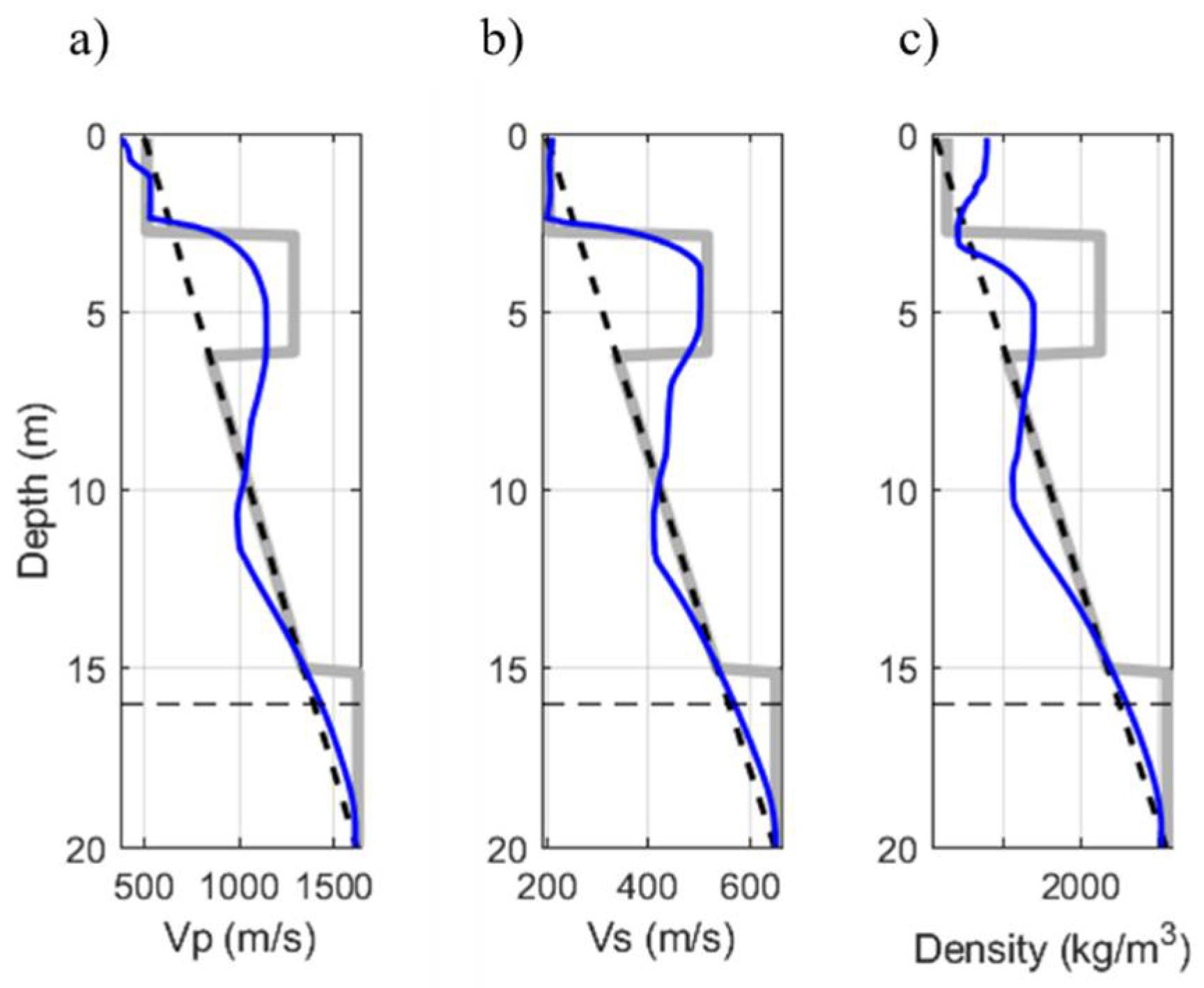
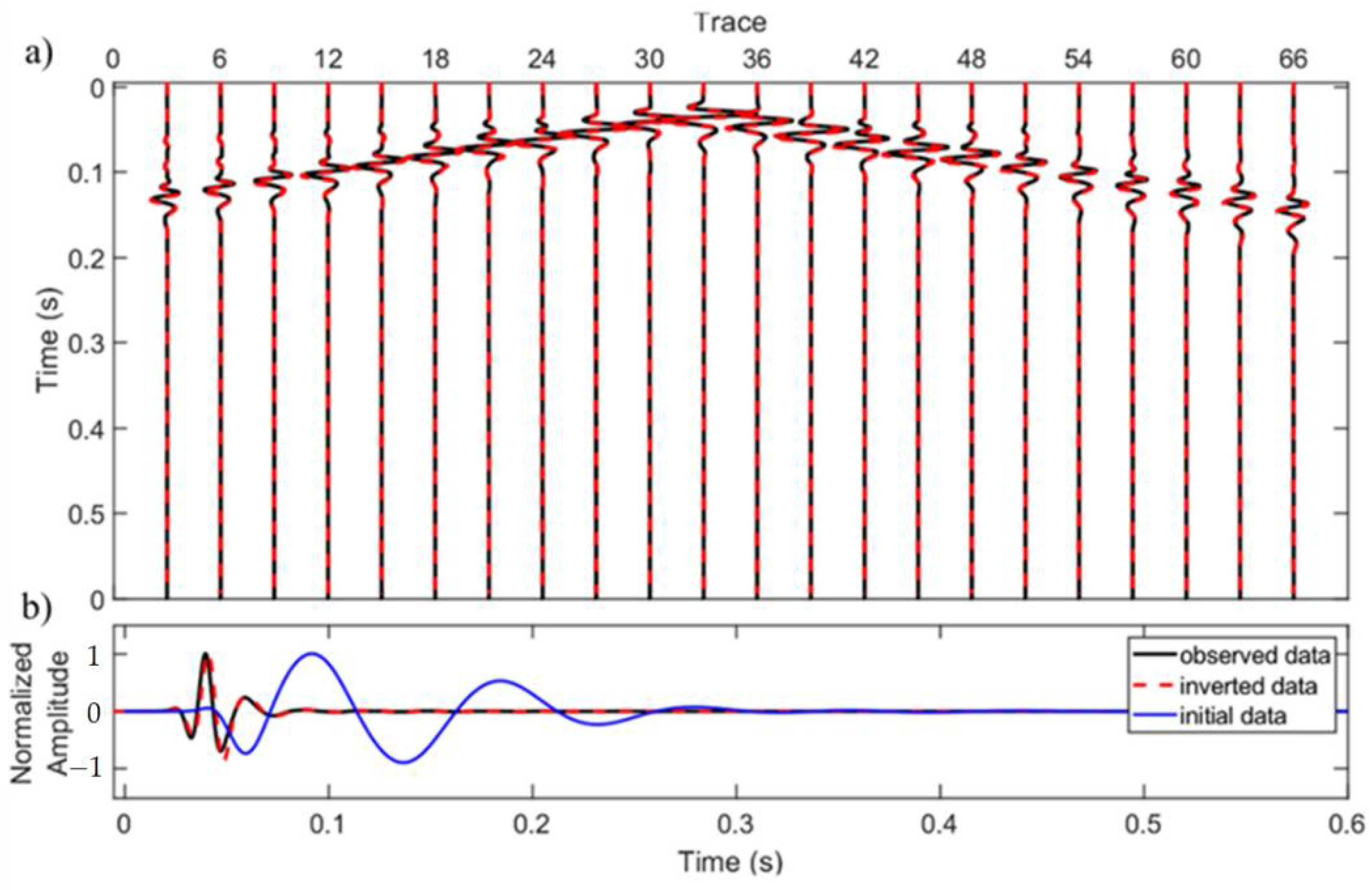
Therefore, it can be said that in this study by considering a broad bandwidth signal as the source wavelet, the capability of the multi-parameter pseudo-viscoelastic FWI of the shallow-seismic wavefield is tested in the case of using a vibroseis source, too. A reflector is then added to the bottom of the true models (Figure 6a, Figure 7a and Figure 8a) at the depth of 15 m. A 1D model is also used for the initial and background of the true models (Figure 6b, Figure 7b and Figure 8b). Multi-parameter inversion is conducted for the parameters discretized at a 2D cartesian grid with the same grid spacing and the total propagation time as were used in the previous example. The high cut frequency filter, up to 100 Hz is applied progressively in the multi-scale strategy. In order to reduce the computational time, the number of receivers was reduced to 66 and the total of shots used in this test is 17. This test takes about 11 hours, and 317 iteration steps are calculated by using the same system as used in the previous test. In this example, the inverted S- wave velocity model (Figure 7c), is still better reconstructed than the P- wave velocity (Figure 6c) and the density (8c) models. The high-velocity layer is reconstructed sharper and more accurate compared to the inverted S- wave velocity model in the previous test. As can be seen in the vertical profile obtained for this model in Figure 9b, the velocity value of the high-velocity layer matches the value of the true high-velocity layer robustly. The velocity value of the low-velocity zone is obtained precisely too. There is an improvement in the results of inversion of the P- wave velocity and density models. As the artefacts in the low-velocity zone are decreased. In the presence of the reflector at the bottom of the model, the structure beneath the high-velocity layer is resolved with higher quality and resolution. In other words, the artefacts at the dipper parts of the models are significantly decreased too. Similar to the previous example, the final synthetic data nicely fits the observed data (Figure 10a). According to the zoomed comparison of the initial and inverted data for trace 36 (Figure 10b), misfit of the inverted and observed data is low.

6. Conclusions

In this study, a 2D multi-parameter pseudo-viscoelastic time domain is applied to a synthetic shallow complex velocity model where a dipping high-velocity layer near the surface with varying thicknesses is used as the case study and both surface and body waves are present. Investigation of these problems requires consideration of various aspects in the presented FWI methods. Some of these aspects that need to be considered in this workflow could be noise contamination, initial velocity model building, elastic and viscoelastic effects, Q factor estimation, and handling long offsets. The other concern about the presented FWI is the convergence speed and computational time of both the forward and inverse steps. Obviously, the size of the velocity model and observed data for near-surface application is not comparable with deep reflection data. The forward modeling step for generating synthetically predicted data from the initial model, back propagation, and computing the gradient, are time consuming steps in the proposed strategy. Thus, to speed up the processing time and increase the converge speed, the nonlinear conjugate gradient method was used. Defining the order of the finite difference operator, discretization, built-in wavelet, Q factor approximation, optimization method, and boundary condition definitions also need to be considered. The first synthetic example shows that when the velocity values in the model are not high, P- wave and S- wave velocity, and density models can be reconstructed well using a low frequency source signal. When the velocity values in the model are higher, the high-velocity layer cannot be resolved with the P- wave velocity model because of the large p-wavelength propagated through the medium. Therefore, the use of a wavelet with a broader bandwidth and higher center frequency can be the solution. In the second experiment, a Ricker wavelet is used to fulfill this issue. Both experiments provide satisfactory and reasonable results as the high-velocity layer near the surface is fairly reconstructed and the structures below this layer are also partially imaged. Reconstruction of the S- wave velocity model is more reliable and accurate compared to p-wave velocity and density models, due to less sensitivity of the surface waves with respect to the P- wave velocity and density parameters. This issue needs to be studied and improved in the future. However, it should be noted that a better image of subsurface structures would be obtained if attenuation of P- and S- waves are inverted simultaneously with the model parameters.

Author Contributions

Conceptualization, N.A., M.S.M. and T.B.; Methodology, T.B.; Software, N.A., M.S.M. and T.B.; Validation, N.A.; Formal analysis, N.A., M.S.M. and T.B.; Data curation, T.B.; Writing—original draft preparation, N.A.; Writing—review and editing, M.S.M.; Supervision, M.S.M., A.R.K. and T.B. All authors have read and agreed to the published version of the manuscript.

Funding

This research received no external funding.

Institutional Review Board Statement

Not applicable.

Informed Consent Statement

Not applicable.

Data Availability Statement

Not applicable.

Conflicts of Interest

The authors declare no conflict of interest.

References

  1. Al-Ali, M.N.; Verschuur, D.J. An integrated method for resolving the seismic complex near-surface problem. Geophys. Prospect. 2006, 54, 739–750. [Google Scholar] [CrossRef]
  2. Soleimani, M. Challenges of seismic imaging in complex media around Iran, from Zagros overthrust in the southwest to Gorgan Plain in the northeast. Lead. Edge 2017, 36, 499–506. [Google Scholar] [CrossRef]
  3. Wittkamp, F.; Athanasopoulos, N.; Bohlen, T. Individual and joint 2-D elastic full-waveform inversion of Rayleigh and Love waves. Geophys. J. Int. 2019, 216, 350–364. [Google Scholar] [CrossRef] [Green Version]
  4. Soleimani, M. Seismic image enhancement of mud volcano bearing complex structure by the CDS method, a case study in SE of the Caspian Sea shoreline. Russ. Geol. Geophys. 2016, 57, 1757–1768. [Google Scholar] [CrossRef]
  5. Soleimani, M. Naturally fractured hydrocarbon reservoir simulation by elastic fractures modeling. Petrol. Sci. 2017, 14, 286–301. [Google Scholar] [CrossRef] [Green Version]
  6. Pan, Y.; Gao, L.; Bohlen, T. Time-domain full-waveform inversion of Rayleigh and Love waves in presence of free-surface topography. J. Appl. Geophys. 2018, 152, 77–85. [Google Scholar] [CrossRef]
  7. Ravaut, C.; Operto, S.; Improta, L.; Virieux, J.; Herrero, A.; Dell’Aversana, P. Multiscale imaging of complex structures from multifold wide-aperture seismic data by frequency-domain full-waveform tomography: Application to a thrust belt. Geophys. J. Int. 2004, 159, 1032–1056. [Google Scholar] [CrossRef] [Green Version]
  8. Brossier, R. Seismic imaging of complex structures by 2D elastic frequency-domain full-waveform inversion. Geophysics 2009, 74, WCC63–WCC76. [Google Scholar] [CrossRef]
  9. Singh, S.; Kanli, A.I.; Mukhopadhyay, S. Full waveform inversion in time and frequency domain of velocity modeling in seismic imaging: FWISIMAT a Matlab code. Earth Sci. Res. J. 2018, 22, 291–300. [Google Scholar] [CrossRef]
  10. Tarantola, A. A strategy for nonlinear inversion of seismic reflection data. Geophysics 1986, 51, 1893–1903. [Google Scholar] [CrossRef]
  11. Soleimani, M. Seismic imaging by 3D partial CDS method in complex media. J. Pet. Sci. Eng. 2016, 143, 54–64. [Google Scholar] [CrossRef]
  12. Choi, Y.; Shin, C. Frequency-domain elastic full waveform inversion using the new pseudo-Hessian matrix: Experience of elastic Marmousi 2 synthetic data. Bull. Seismol. Soc. Am. 2008, 98, 2402–2415. [Google Scholar] [CrossRef]
  13. Martin, G.S.; Wiley, R.; Marfurt, K.J. Marmousi2: An elastic upgrade for Marmousi. Lead. Edge 2006, 25, 156–166. [Google Scholar] [CrossRef]
  14. Choi, Y.; Min, D.; Shin, C. Two-dimensional waveform inversion of multi-component data in acoustic elastic coupled media. Geophys. Prospect. 2008, 56, 863–881. [Google Scholar] [CrossRef]
  15. Brossier, R.; Virieux, J.; Operto, S. Parsimonious finite-volume frequency-domain method for 2-D P-SV-wave modelling. Geophys. J. Int. 2008, 175, 541–559. [Google Scholar] [CrossRef] [Green Version]
  16. Thiel, N.; Bohlen, T. 2d Acoustic Full Waveform Inversion of Submarine Salt Layer Using Dual Sensor Streamer Data; Annual WIT Report; Annual WIT: Hamburg, Germany, 2016. [Google Scholar]
  17. Brossier, R. Two-dimensional frequency-domain visco-elastic full waveform inversion: Parallel algorithms, optimization and performance. Comput. Geosci. 2011, 37, 444–455. [Google Scholar] [CrossRef]
  18. Kurzmann, A.; Gaßner, L.; Shigapov, R.; Thiel, N.; Athanasopoulos, N.; Bohlen, T.; Steinweg, T. Real data applications of seismic full waveform inversion. In High Performance Computing in Science and Engineering’17; Springer: Cham, Switzerland, 2018; pp. 467–484. [Google Scholar]
  19. Gao, L.; Pan, Y.; Bohlen, T. 2-D multiparameter viscoelastic shallow-seismic full-waveform inversion: Reconstruction tests and first field-data application. Geophys. J. Int. 2020, 222, 560–571. [Google Scholar] [CrossRef]
  20. Groos, L.; Schäfer, M.; Forbriger, T.; Bohlen, T. The role of attenuation in 2D full-waveform inversion of shallow-seismic body and Rayleigh waves. Geophysics 2014, 79, R247–R261. [Google Scholar] [CrossRef]
  21. Groos, L.; Schäfer, M.; Forbriger, T.; Bohlen, T. Application of a complete workflow for 2D elastic full-waveform inversion to recorded shallow-seismic Rayleigh waves. Geophysics 2017, 82, R109–R117. [Google Scholar] [CrossRef]
  22. Bohlen, T.; Wittkamp, F. Three-dimensional viscoelastic time-domain finite-difference seismic modelling using the staggered Adams–Bashforth time integrator. Geophys. J. Int. 2016, 204, 1781–1788. [Google Scholar] [CrossRef] [Green Version]
  23. Butzer, S.; Kurzmann, A.; Bohlen, T. 3D elastic full-waveform inversion of small scale heterogeneities in transmission geometry. Geophys. Prospect. 2013, 61, 1238–1251. [Google Scholar] [CrossRef]
  24. Jetschny, S.; Bohlen, T.; Kurzmann, A. Seismic prediction of geological structures ahead of the tunnel using tunnel surface waves. Geophys. Prospect. 2011, 59, 934–946. [Google Scholar] [CrossRef]
  25. Robertsson, J.O.; Levander, A.; Symes, W.W.; Holliger, K. A Comparative Study of Free-Surface Boundary Conditions for Finite-Difference Simulation of Elastic/Viscoelastic Wave Propagation. In SEG Technical Program Expanded Abstracts; SEG library: Houston, TX, USA, 1995; pp. 1277–1280. [Google Scholar]
  26. Blanch, J.O.; Robertsson, J.O.A.; Symes, W.W. Modeling of a constant Q: Methodology and algorithm for an efficient and optimally inexpensive viscoelastic technique. Geophysics 1995, 60, 176–184. [Google Scholar] [CrossRef] [Green Version]
  27. Bohlen, T. Parallel 3-D viscoelastic finite difference seismic modeling. Comput. Geosci. 2002, 28, 887–899. [Google Scholar] [CrossRef]
  28. Groos, L. 2D Full Waveform Inversion of Shallow Seismic Rayleigh Waves. Ph.D Thesis, Karlsruher Institut für Technologie (KIT), Karlsruhe, Germany, 2013. [Google Scholar]
  29. Komatitsch, D.; Martin, R. An unsplit convolutional perfectly matched layer improved at grazing incidence for the seismic wave equation. Geophysics 2007, 72, SM155–SM167. [Google Scholar] [CrossRef]
  30. Martin, R.; Komatitsch, D. An unsplit convolutional perfectly matched layer technique improved at grazing incidence for the viscoelastic wave equation. Geophys. J. Int. 2009, 179, 333–344. [Google Scholar] [CrossRef] [Green Version]
  31. Choi, Y.; Alkhalifah, T. Application of multi-source waveform inversion to marine streamer data using the global correlation norm. Geophys. Prospect. 2012, 60, 748–758. [Google Scholar] [CrossRef]
  32. Köhn, D. Time Domain 2D Elastic Full Waveform Tomography. Ph.D. Thesis, Christian-Albrechts-Universität zu Kiel, Kiel, Germany, 2011. [Google Scholar]
  33. Sourbier, F.; Operto, S.; Virieux, J.; Amestoy, P.; L’Excellent, J.Y. FWT2D: A massively parallel program for frequency-domain full-waveform tomography of wide-aperture seismic data—Part 1: Algorithm. Comput. Geosci. 2009, 35, 487–495. [Google Scholar] [CrossRef]
  34. Sourbier, F.; Operto, S.; Virieux, J.; Amestoy, P.; L’Excellent, J.Y. FWT2D: A massively parallel program for frequency-domain full-waveform tomography of wide-aperture seismic data—Part 2: Numerical examples and scalability analysis. Comput. Geosci. 2009, 35, 496–514. [Google Scholar] [CrossRef]
  35. Brossier, R. Imagerie Sismique à deux Dimensions des Milieux Visco-Élastiques par Inversion des Formes D’ondes: Développements Méthodologiques et Applications. Ph.D. Thesis, Université Nice Sophia Antipolis, Nice, France, 2009. [Google Scholar]
  36. Soleimani, M.; Rafie, M. Imaging of seismic data in complex structures by introducing the partial diffraction surface stack method. Studia Geophys. Geod. 2016, 60, 644–661. [Google Scholar] [CrossRef]
  37. Mora, P. Nonlinear two-dimensional elastic inversion of multioffset seismic data. Geophysics 1987, 52, 1211–1228. [Google Scholar] [CrossRef]
  38. Tarantola, A. Theoretical background for the inversion of seismic waveforms, including elasticity and attenuation. Pure Appl. Geophys. 1988, 128, 365–399. [Google Scholar] [CrossRef]
  39. Plessix, R.E.; Mulder, W.A. Frequency-domain finite-difference amplitude-preserving migration. Geophys. J. Int. 2004, 157, 975–987. [Google Scholar] [CrossRef]
  40. Bunks, C.; Saleck, F.M.; Zaleski, S.; Chavent, G. Multiscale seismic wave-form inversion. Geophysics 1995, 60, 1457–1473. [Google Scholar] [CrossRef]
  41. Kamberis, E.; Kokinou, E.; Koci, F.; Lioni, K.; Alves, T.M.; Velaj, T. Triassic evaporites and the structural architecture of the External Hellenides and Albanides (SE Europe): Controls on the petroleum and geoenergy systems of Greece and Albania. Int. J. Earth Sci. 2022, 111, 789–821. [Google Scholar] [CrossRef]
  42. Roure, F.; Andriessen, P.; Callot, J.P.; Faure, J.L.; Ferket, H.; Gonzales, E.; Guilhaumou, N.; Lacombe, O.; Malandain, J.; Sassi, W.; et al. The Use of Palaeo-Thermo-Barometers and Coupled Thermal, Fluid Flow and Pore-Fluid Pressure Modelling for Hydrocarbon and Reservoir Prediction in Fold and Thrust Belts; Book chapter; Geological Society Publications: London, UK, 2010; Volume 348. [Google Scholar]
  43. Socco, L.V.; Foti, S.; Boiero, D. Surface-wave analysis for building near-surface velocity models -Established approaches and new perspectives. Geophysics 2010, 75, 75A83–75A102. [Google Scholar] [CrossRef]
  44. Athanasopoulos, N.; Manukyan, E.; Bohlen, T.; Maurer, H. Accurate reconstruction of shallow P-wave velocity model with time-windowed elastic full-waveform inversion. In Proceedings of the 80th EAGE Conference and Exhibition 2018, Copenhagen, Denmark, 11–14 June 2018; pp. 1–5. [Google Scholar]
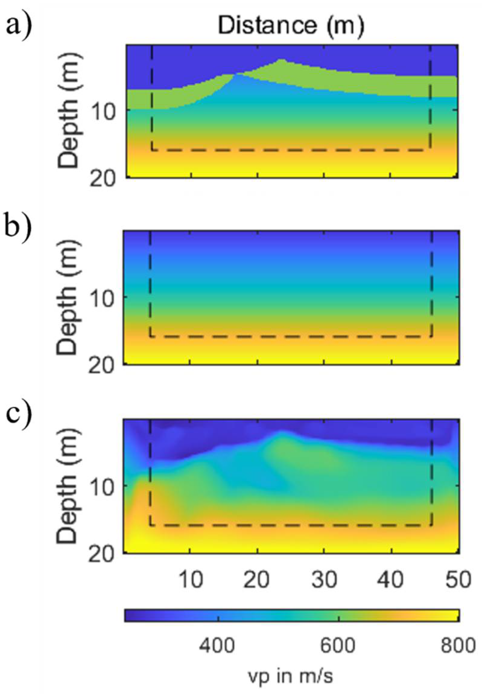
Figure 1. Multi-parameter synthetic example when using a low-frequency source signal: (a) the true P- wave velocity model for the calculation of the observed data, (b) the initial P- wave velocity model, and (c) the inverted P- wave velocity model. The CPML frame is marked by a thin black line.
Applsci 12 07741 g001
Figure 2. Multi-parameter synthetic example when using a low-frequency source signal: (a) the true S- wave velocity model for the calculation of the observed data, (b) the initial S- wave velocity model, and (c) the inverted S- wave velocity model. The CPML frame is marked by a thin black line.
Applsci 12 07741 g002
Figure 3. Multi-parameter synthetic example when using a low-frequency source signal: (a) the true density model for the calculation of the observed data, (b) the initial density model, and (c) the inverted density model. The CPML frame is marked by a thin black line.
Applsci 12 07741 g003
Figure 4. Model fitting when using a low-frequency source signal: (a) vertical profiles of the P- wave velocity model, (b) vertical profiles of the S- wave velocity model, and (c) vertical profiles of the density model. The true model is plotted with the grey line, the initial model is represented by the dashed black line and vertical profile at x = 25   m of the inverted models is the plotted blue line.
Applsci 12 07741 g004
Figure 5. Fitting of the data in the shot at x = 9 m when using a low-frequency source signal. (a) Comparison of the vertical velocity observed and inverted seismograms. (b) Comparison of the normalized seismograms calculated for the initial, inverted, and observed data for trace 36.
Applsci 12 07741 g005
Figure 6. Multi-parameter synthetic example when using a high-frequency source signal: (a) the true P- wave velocity model for the calculation of the observed data, (b) the initial P- wave velocity model, and (c) the inverted P- wave velocity model. The CPML frame is marked by a thin black line.
Applsci 12 07741 g006
Figure 7. Multi-parameter synthetic example when using a high-frequency source signal: (a) the true S- wave velocity model for the calculation of the observed data, (b) the initial S- wave velocity model, and (c) the inverted S- wave velocity model. The CPML frame is marked by a thin black line.
Applsci 12 07741 g007
Figure 8. Multi-parameter synthetic example when using a high-frequency source signal: (a) the true density model for the calculation of the observed data, (b) the initial density model, and (c) the inverted density model. The CPML frame is marked by a thin black line.
Applsci 12 07741 g008
Figure 9. Model fitting when using a high-frequency source signal: (a) vertical profiles of the P- wave velocity model, (b) vertical profiles of the S- wave velocity model, (c) vertical profiles of the density model. The true model is plotted with the grey line, the initial model is represented by the dashed black line and vertical profile at x = 25   m of the inverted models is the plotted blue line.
Applsci 12 07741 g009
Figure 10. Fitting of the data in the shot at x = 9 m when using a high-frequency source signal. (a) Comparison of the vertical velocity observed and inverted seismograms. (b) Comparison of the normalized seismograms calculated for the initial, inverted, and observed data for trace 36.
Applsci 12 07741 g010
Publisher’s Note: MDPI stays neutral with regard to jurisdictional claims in published maps and institutional affiliations.