Regimes in the Response of Photomechanical Materials

Abstract

Photomechanical materials perform mechanical work in response to illumination. Photoisomerization-based photomechanical materials may operate in different regimes depending on the intensity of the illuminating light. We examine the photoresponse of liquid crystalline azo-acrylate networks and show that a material property, the characteristic intensity of the material, defines the boundaries between different regimes. Asymptotic analysis indicates that whereas at low relative light levels, photostress is proportional to intensity, at high levels, it is proportional to fluence. Model predictions are in good agreement with the experimental results.

1. Introduction

Photomechanical materials are under intense current scrutiny to assess their suitability for the direct conversion of light into mechanical work. Of particular interest are materials containing or consisting of photoisomerizable molecules [1,2,3,4,5]. In this work, we focus on azo-dye-doped nematic liquid crystal networks/elastomers but expect that our approach may be applicable to a broad range of photoisomerizable materials [6]. Key to effective utilization of these materials is the efficient photoisomerization of the azo-acrylate molecules in the network. Although it is clear that it is the energy of the absorbed light that ultimately delivers the photowork, it is less clear what intensity of illumination best accomplishes this. It is known from the work of Warner [7,8] that there exists a material parameter with the units of intensity that set the scale. Here we give an explicit definition of this critical intensity, measure the parameters that allow its experimental determination and then carry out experiments to compare model predictions based on this critical intensity with observed results.

It is often assumed that the photostrain depends on light intensity [9,10,11,12,13], or the number density of the cis molecules is a function of light intensity [14]. We show that, instead, the photostrain depends on light intensity only when the light intensity is small. When the light intensity is large, the system saturates, and the response is to fluence rather than intensity.

In Section 2, we begin with a simple description of such a system, an azo-acrylate network, in order to define the relevant physical parameters. We introduce the dynamics of the azo isomer population. We perform asympotics on this and identify three regimes of intensity with different photoresponse. In Section 3, we measure the cis-lifetime and trans- absorption cross-section, and from these, we determine the characteristic intensity. We then present recent new and unexpected experimental results in Section 4, which suggest a new perspective to better understand the photomechanical response of these materials. We close with a brief summary of our results in Section 5.

2. Light Intensity and Photoisomerization Dynamics

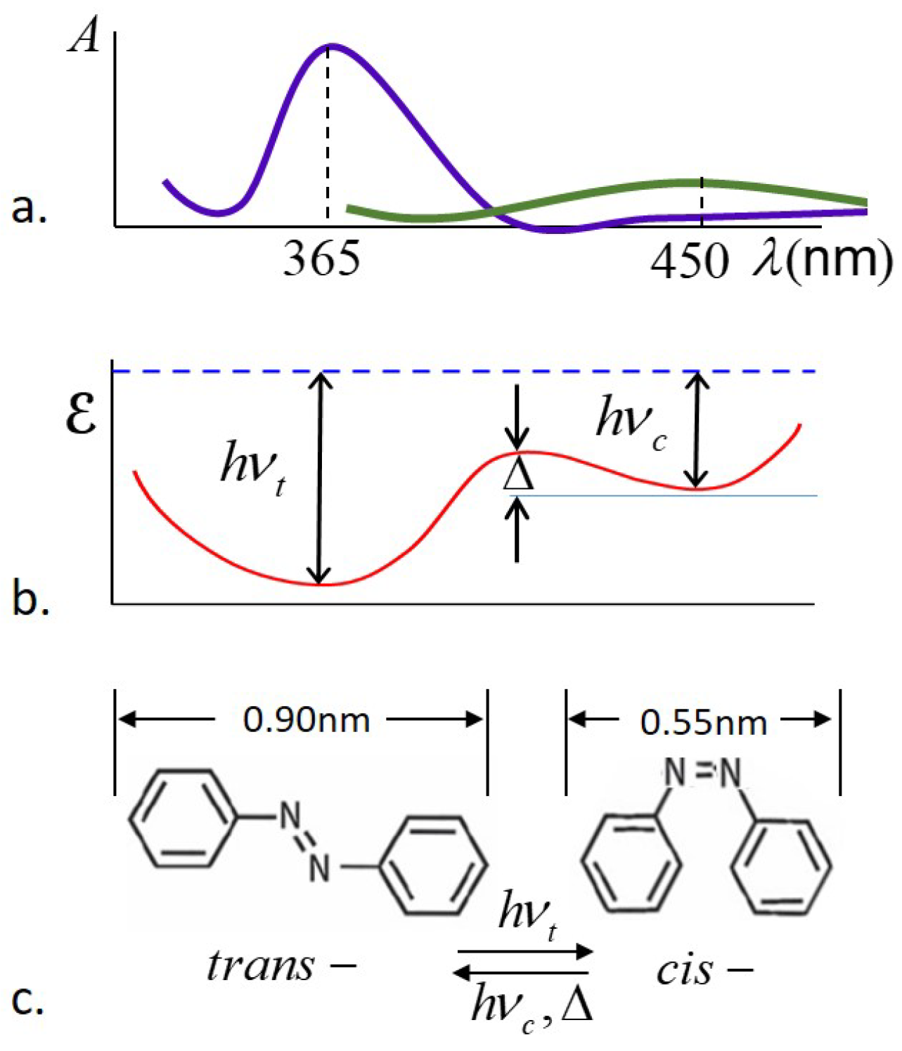
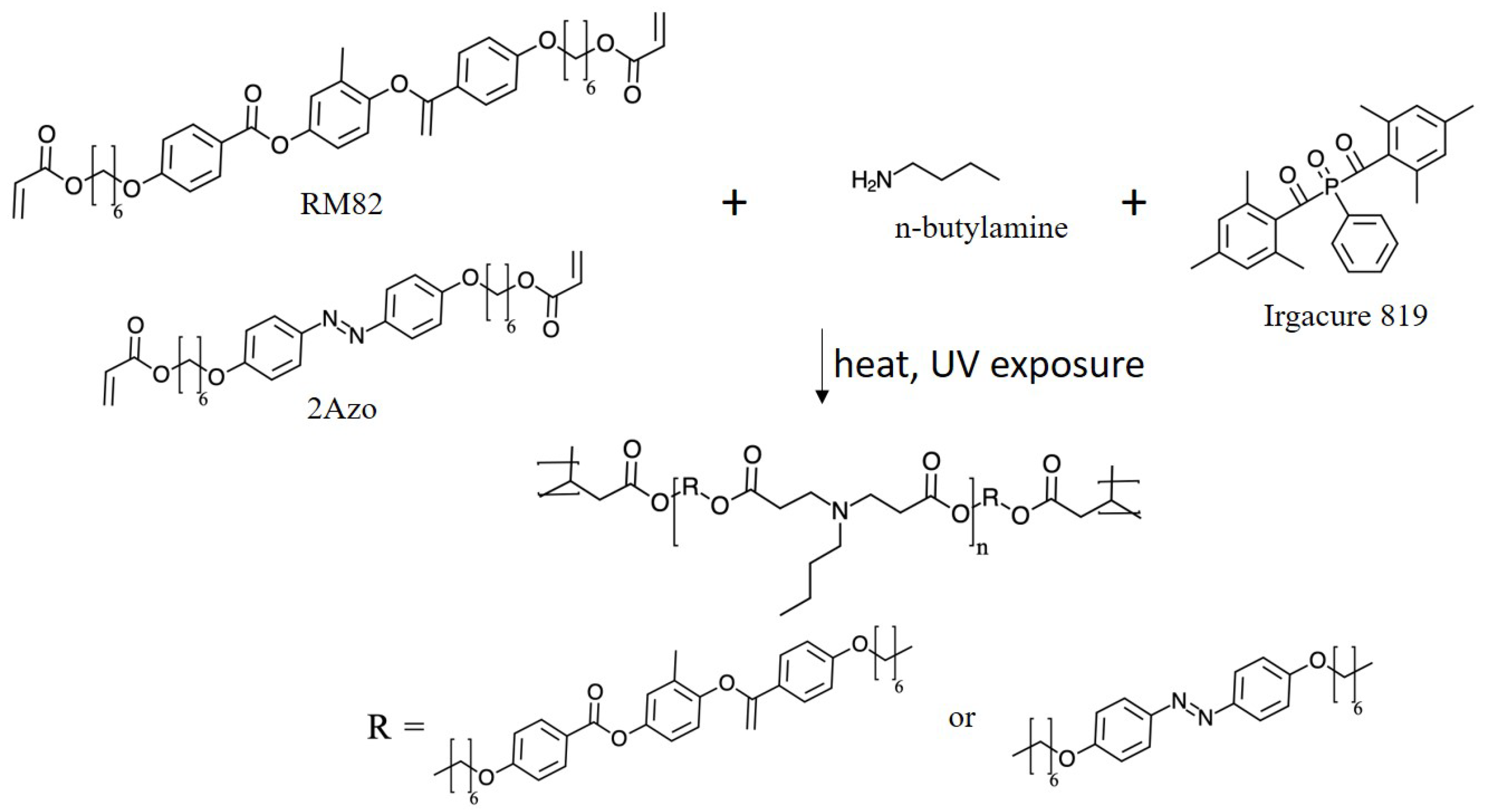
The system under consideration consists of a polymer network formed by cross-linked chains consisting of liquid crystal-forming mesogenic units and photoisomerizable azo dyes. A schematic of one system studied, and the molecular structure of its constituents are shown in Figure 1. The relative quantities of the constituents are given in

Table 1. The relative quantities of the constituents.

	RM82	2 Azo	Acrylates to Amine	Irgacure
	Molar Fraction	Molar Fraction	Molar Ratio	819
Sample	$1-x$	x	$1.1$	$2.5$ wt%

.

The sample shape considered is a rectangular film, consisting of the material in the nematic phase, where the director $\hat{\mathbf{n}}$, the direction of average orientation of the mesogenic units, is in the plane of the film, parallel to the long edge. The azo dye units, which can be either in the elongated low-energy trans-isomer state or the more compact high-energy cis-isomer state, are randomly distributed throughout the sample. It is assumed that the trans-isomers are aligned along the nematic director $\hat{\mathbf{n}}$, while the cis-isomers are assumed to be unaligned, effectively spherical in shape and randomly oriented. The key notion is that photons with energy $h\nu$, where h is Planck’s constant and $\nu$ is the frequency of peak UV absorption by the trans-isomers, are absorbed by the trans-isomers, which then undergo photoisomerization to the cis-form. The shape change of the azo dye constituents results in a shape change of the entire sample, and due to this shape change, the sample is capable of exerting pressure and performing mechanical work on a load. Due to thermal excitations, the photoexcited cis-isomers have a lifetime $\tau$, after which they decay back to the low-energy trans-form. It is assumed that the rate of thermal excitation from trans-to cis-form is essentially negligible, but thermal excitation drives the cis- to trans-isomerization. A schematic of the absorbance, energy landscape, and the corresponding molecular shapes for the trans- and cis-isomers is shown in Figure 2.

Denoting the number densities of the trans- and cis-isomers and a total number of dye molecules by ${\rho }_t$, ${\rho }_c$ and ${\rho }_0$, we have

$${\rho }_t+{\rho }_c={\rho }_0.$$

(1)

If the sample is illuminated by normally incident UV, then the number densities depend on time t and position x in the sample, where x is measured along the normal film surface. The dynamics of the system are given by

$$\frac{\mathrm{\partial }{\rho }_t}{\mathrm{\partial }t}=-I\frac{{\rho }_t{\sigma }^a}{h\nu }+\frac{{\rho }_c}{\tau },$$

(2)

where $I(x, t)$ is the UV light intensity, $\nu$ is the peak absorption frequency, and ${\sigma }^a$ is the absorption cross-section of the trans-isomers.

It is useful to define the characteristic intensity (The characteristic intensity was identified by Warner [7,8], but its relation to material parameters has not been previously given explicitly.) $I_0$, a material parameter, as

$$I_0=\frac{h\nu }{{\sigma }^a\tau },$$

(3)

which sets the scale of the photoexcitation. This corresponds to a characteristic photon number density of

$${\rho }_0^{photon}=\frac{1}{c{\sigma }^a\tau }=\frac{I_0}{ch\nu },$$

(4)

where c is the speed of light.

The dependence of intensity on distance is given by

$$\frac{\partial I}{\partial x}=-I{\rho }_t{\sigma }^a.$$

(5)

It is also useful to define a decay length $l_d$ as

$$l_d=\frac{1}{{\rho }_0{\sigma }^a},$$

(6)

in terms of the total dye number density. As can be seen from Equation (2), the system behavior is determined by the characteristic intensity $I_0$ and the cis-decay time $\tau$.

The dynamical equations of the system, in dimensionless form, are

$$\frac{\partial {\rho }_t}{\partial t}=-{\rho }_t(I+1)+1,$$

(7)

and

$$\frac{\partial I}{\partial x}=-I{\rho }_t,$$

(8)

where the intensity I is measured in units of $I_0$, distance x in units of $l_d$, time t in units of $\tau$, and number density $\rho$ in units of ${\rho }_0$. The coupled equations, Equations (7) and (8), describe the spatial and temporal evolution of the system. We remark here that four material parameters: the cis-lifetime $\tau$, the trans-absorption cross-section ${\sigma }^a$, the energy $h\nu$ absorbed by trans-isomer, and the dye number density ${\rho }_0$ are needed to describe the dynamics of a specific system. The shape change of the sample is the result of the shape change of the dye molecules; the quantity of primary interest is, therefore, ${\rho }_c$, the number density of dye molecules excited into the cis-state, which we assume to be proportional to the photostress.

The total absorbed energy per volume by the sample to reach the time-independent photostationary state in dimensional units is

$${\mathcal{E}}_p\simeq \frac{1}{d}{\int }_0^d{\int }_0^{{\tau }_p}I{\rho }_t{\sigma }^{a}dxdt,$$

(9)

where ${\tau }_p$ is the time to reach the photostationary state.

Since there is no closed-form analytic solution of the dynamical equations, we look at the behavior asymptotically.

Asymptotic Dynamics

In general, the intensity I varies with time because ${\rho }_t$ changes with time. However, our numerical experiments suggest that keeping the intensity invariant with time would not result in a large discrepancy in ${\rho }_t$. This implies that we can treat the intensity as a constant in time (This is reasonable for samples thin compared to the absorption length $l_d$.), which enables us to make qualitative estimates of the dye dynamics. In dimensionless quantities, Equation (7) can be integrated to give

$${\rho }_t=\frac{1}{I+1}(1+I{e}^{-(I+1)t}),$$

(10)

where the constant of integration has been chosen so that ${\rho }_t(x, 0)=1$; that is, all dyes are in the trans-state initially. It follows that

$${\rho }_c=\frac{I}{I+1}(1-e^{-(I+1)t}),$$

(11)

and the system approaches the steady-state exponentially. Early; that is, when $t \ll 1/(I + 1)$, we have that

$${\rho }_c\simeq It,$$

(12)

and the cis-number density ${\rho }_c$ is proportional to the fluence of the incident light.

The characteristic intensity plays a key role in the system response. Depending on the intensity, three different regimes can be distinguished.

Regime 1. If $I \ll 1$, then the cis-number density ${\rho }_c$ is

$${\rho }_c\simeq I(1-e^{-t}).$$

(13)

The time to reach the photostationary state is $t \approx 1$, or, in dimensional units, $\tau$ seconds. In the photostationary state,

$${\rho }_c\simeq I$$

(14)

and the photostress is proportional to the intensity. If the illumination is removed, the cis-population will decay with the time constant $\tau$ seconds; at the same rate as to reach the photostationary state. The total absorbed energy per volume by the sample to reach the photostationary state, from Equation (9), is ${\mathcal{E}}_p\simeq {\rho }_0\frac{I}{I_0}h\nu$ in dimensional units, and in this regime, the absorbed energy is $h\nu$ per molecule for the fraction $I/I_0$ of dye molecules.

Regime 2. If $I \approx 1$, then the cis-number density ${\rho }_c$ is

$${\rho }_c\simeq \frac{I}{I+1}(1-e^{-(I+1)t}).$$

(15)

The time to reach the photostationary state is $t \approx 1/(I + 1)$, or, in dimensional units, $\tau /(I/I_0+1)$ seconds. In the photostationary state,

$${\rho }_c\approx \frac{I}{I+1}.$$

(16)

If the illumination is removed, the cis-population will decay with time constant $\tau$ seconds; a factor of $I + 1$ slower than to reach the photostationary state. The total absorbed energy per volume by the sample to reach the photostationary state, in dimensional units, is ${\mathcal{E}}_p\simeq \frac{1}{I/I_0+1}{\rho }_{0}h\nu$, and in this regime, the absorbed energy is $h\nu$ per molecule for the fraction $\frac{1}{I/I_0+1}$ of dye molecules.

Regime 3. If $I \gg 1$, then the cis-number density ${\rho }_c$ is

$${\rho }_c\simeq 1-e^{-It}.$$

(17)

The time to reach the photostationary state is $t \approx 1/I$, or, in dimensional units, $\tau /(I/I_0)$ seconds. In the photostationary state,

$${\rho }_c=\frac{I}{I+1}\simeq 1,$$

(18)

and

$${\rho }_t\simeq 0.$$

(19)

If the illumination is removed, the cis-population will decay with time constant $\tau$ seconds; a factor $I/I_0$ slower than to reach the photostationary state. The total absorbed energy per volume by the sample to reach the photostationary state, in dimensional units, is $\mathcal{E}\simeq {\rho }_{0}h\nu$, and in this regime, the absorbed energy is $h\nu$ per every dye molecule.

The key difference among the three regimes is the difference in the cis-populations, and the difference in times to reach the photostationary state. In regime 1, $I \ll 1$, ${\rho }_c \simeq 0$, ${\rho }_t$$\simeq 1$, while in regime 3, $I \gg 1$, ${\rho }_c \simeq 1$, ${\rho }_t$$\simeq 0$.

3. Material Parameters

As we pointed out in Section 2, key parameters that determine the photoisomer populations and hence the response of the system are $h\nu , {\rho }_0, {\sigma }^a$, and $\tau$. We have determined these experimentally, as discussed below.

The number density ratio of the trans- and cis-isomers in the absence of illumination can be estimated. First, at 365 nm, $h\nu = 5.45 \times {10}^{-19}$ J = 3.4 eV. The energy difference between trans- and cis-isomers is approximately $h\nu /10$. At room temperature, ${\rho }_c/{\rho }_t \approx {10}^{-6}$, ${\rho }_t \approx {\rho }_0$ and, without photoexcitation, essentially all dye molecules are in the trans state.

The number density of azo dye molecules, regardless of isomerization, can be estimated as follows. If the mass density of azo dye is comparable to that of water, then $1\mathrm{mol}$ of dye has a volume of 551 cm³, and the number density ${\rho }_0$ is $1.1 \times {10}^{27}$/m³ for pure azo dye. For typical mixtures with 10 wt% azo, we then estimate the dye number density to be ${\rho }_0 \simeq {10}^{26}$/m³ and recognize that the margin of error may be as large as one order of magnitude.

The absorption cross-section can be estimated from the absorbance if the dye number density is known. For a 10 $\mathsf{\mu }$m sample with 5 mol% dye, the measured absorbance at 365 nm is $1.3$. The transmittance T is $e^{-1.3} = 0.272$, and since we expect that, at low intensity,

$$I=I_i{e}^{-x/l_d},$$

(20)

we have that the absorption length is $l_d={10}^{-5}/1.3$ m = 7.7 $\mathsf{\mu }$m. From Equation (6) we obtain

$${\sigma }^a=\frac{1}{{\rho }_0{l}_d}={10}^{-21} {\mathrm{m}}^2.$$

(21)

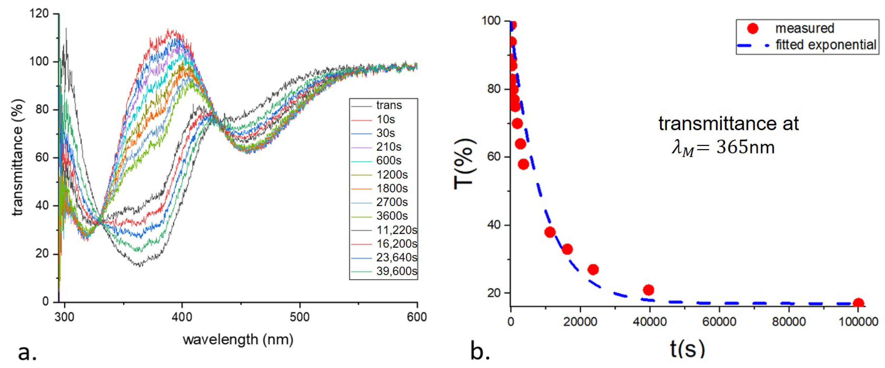
The relaxation time was obtained by measuring the transmittance of the photoexcited sample as a function of time. The transmittance, normalized to that of an identical but undyed sample, is shown in Figure 3a. The decay time $\tau$ is 9030 s.

The characteristic intensity can now be calculated as

$$I_0=\frac{h\nu }{{\sigma }^a\tau }\simeq \frac{{10}^{-18}}{{10}^{-21}\times {10}^4}=0.1 \mathrm{W}/{\mathrm{m}}^2.$$

(22)

The estimate for $I_0$ can be confirmed experimentally. For light traversing the sample in the photostationary state, from Equations (7) and (8), we write [8],

$$I_0=\frac{I_i(1-T)}{lnT+d{\rho }_0{\sigma }^a}.$$

(23)

For incident light at 365 nm and using an attenuator to achieve low intensity, the incident intensity $I_i$ was $0.05$ mW/cm², (We use the units mW/cm² from here on to enable ready comparison with the values in the literature.) and the transmittance T of the photoisomerized sample was $0.8$. This gives $I_0=0.013$ mW/cm², in agreement with our earlier estimate. In

Table 2. Material parameters of the azo-acrylate system.

Number Density	Decay Length	Absorption	cis-Lifetime	Characteristic
of Dye		Cross-Section		Intensity
${\rho }_0$ (m−3)	$l_d$ (m)	${\sigma }^a$ (m2)	$\tau$ (s)	$I_0$ (W/m2)
${10}^{26}$	${10}^{-5}$	${10}^{-21}$	${10}^4$	${10}^{-1}$

, we summarize our results for the material parameters of the azo-acrylate system studied.

Expected Impact on Experiments

Typical UV intensities in use in experiments on azo-acrylic systems are $I = 100$ mW/cm² [12,16,17,18,19,20,21] or similar [22,23]. Since we have determined that $I_0 = 0.01$ mW/cm², this corresponds to

$$\frac{I}{I_0}={10}^4,$$

(24)

a remarkably large value, placing the systems firmly in regime 3. The time to reach the photostationary state is, therefore,

$$t=\frac{\tau }{(I/I_0)}=1\mathrm{s}.$$

(25)

We expect, therefore, saturation of the photoresponse on this timescale, as well as energy absorption corresponding to $h\nu$ per dye molecule.

4. Experimental Results

We carried out experiments on samples (E) obtained from the Eindhoven group of D. Liu and D. Broer and on samples (K) synthesized at Kent. The samples were rectangular strips, with E-type samples 5 mm wide and 10 $\mathsf{\mu }$m thick, with 0 and 5 mol% azo and elastic modulus $Y \simeq 100$ MPa, while K-type samples were 5 mm wide and 25 $\mathsf{\mu }$m thick, with 0 and 2 mol% azo and elastic modulus Y$\simeq 60$ MPa. Typical sample lengths varied from 5 to 20 mm.

To our knowledge, samples with our compositions are not commercially available. The samples used were either synthesized by the group of D. Liu and D. Broer or by us. Some information on synthesis is provided in [18,24,25].

We note here that samples were held by specially designed endpieces, two parallel plexiglass strips held together by a miniature nylon bolt and nuts at each end. These were attached to the top and bottom edges of the vertically held samples. The bottom endpiece was rigidly held in place by two fingers on a metal arm supported by the optical table below. The top endpiece was attached either to an Entran force sensor or to a balance arm via a stiff thread. Since the top and bottom endpieces fit snugly against the flat front of the arm, the sample cannot rotate. The anticipated and observed photoresponse of the samples consisted either of no observable change of shape (photostress measurements) or observed linear contraction (photostrain measurements). Changes in width or thickness were too small to observe and were not measured.

4.1. Photostress

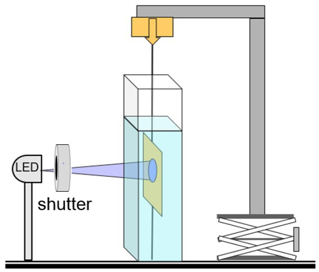
We carried out photostress measurements by holding the 5 mm top and bottom ends of the rectangular strips of sample materials fixed and measured the force exerted by the sample on illumination. The nematic director was parallel to the long vertical edge of the samples. The photostress produced by the samples was measured both in air and in water, the latter in order to maintain (nearly) constant temperature. Photomechanical forces were measured by an Entran force sensor attached to the top edge of the samples. Data were collected using NI LabVIEW. A schematic of the setup is shown in Figure 4.

The light source was a high-powered LED at 365 nm calibrated with a Scientech H410 power meter. The top and bottom edges of the samples were clamped in thin plexiglass sample holders, which were attached to the optical table below (details not shown) and to the Entran force sensor on top via a 100 $\mathsf{\mu }$m outside diameter nearly inextensible filament (Fireline jewelry thread). To probe details of the photoresponse, instead of using continuous illumination, samples were photoexcited by 200 ms pulses of UV light, followed by 1 s of darkness, using a shutter. 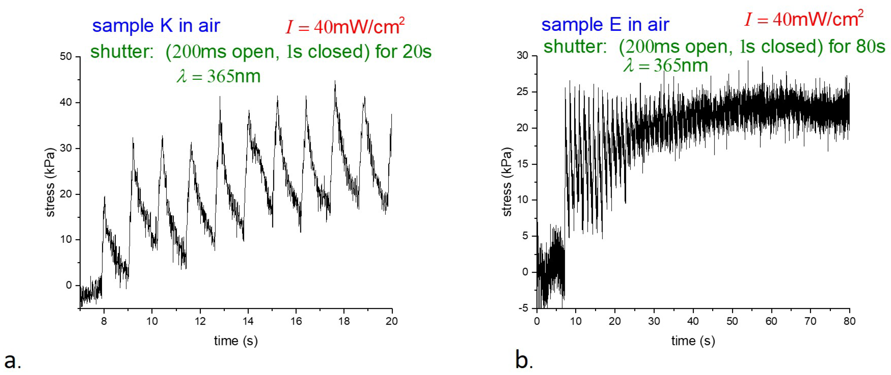The photostress in air is shown in Figure 5.

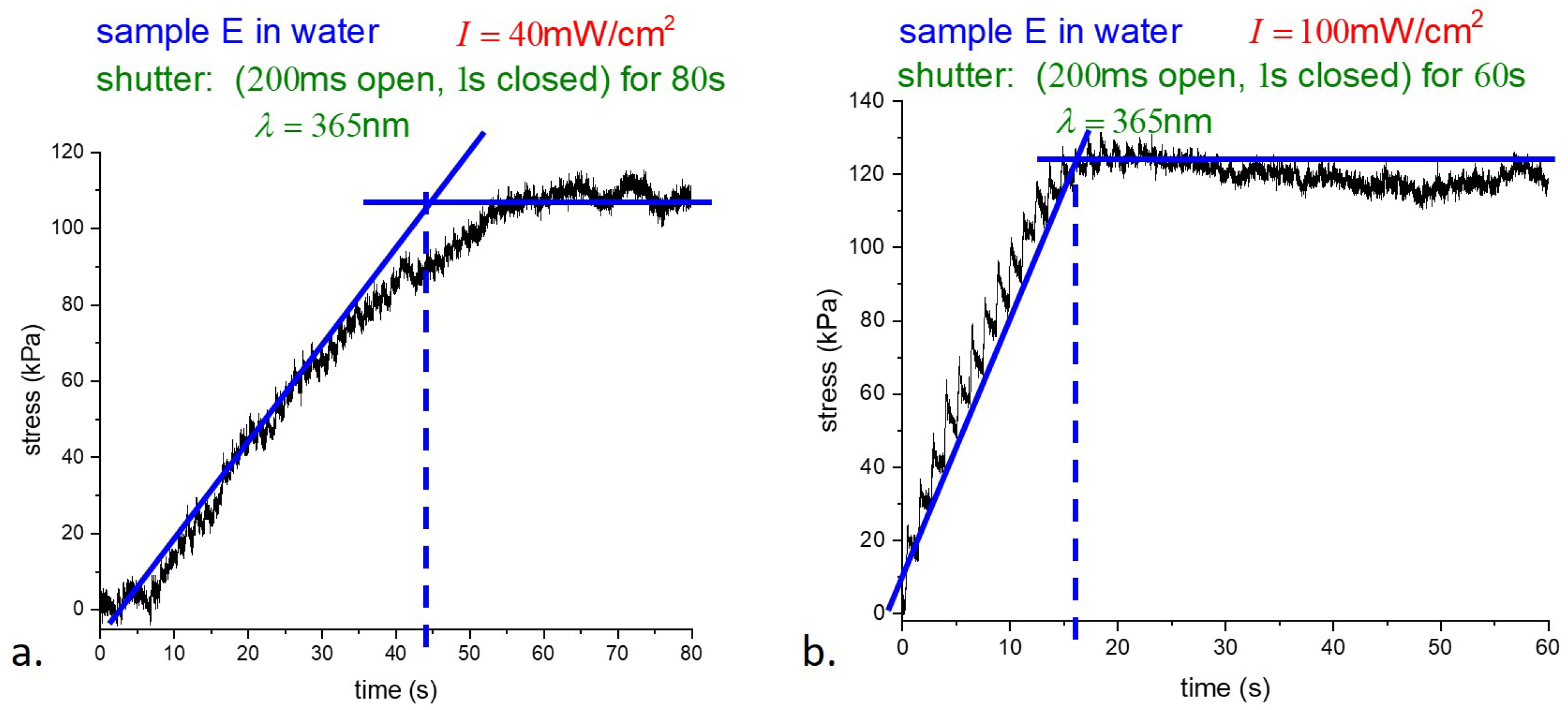
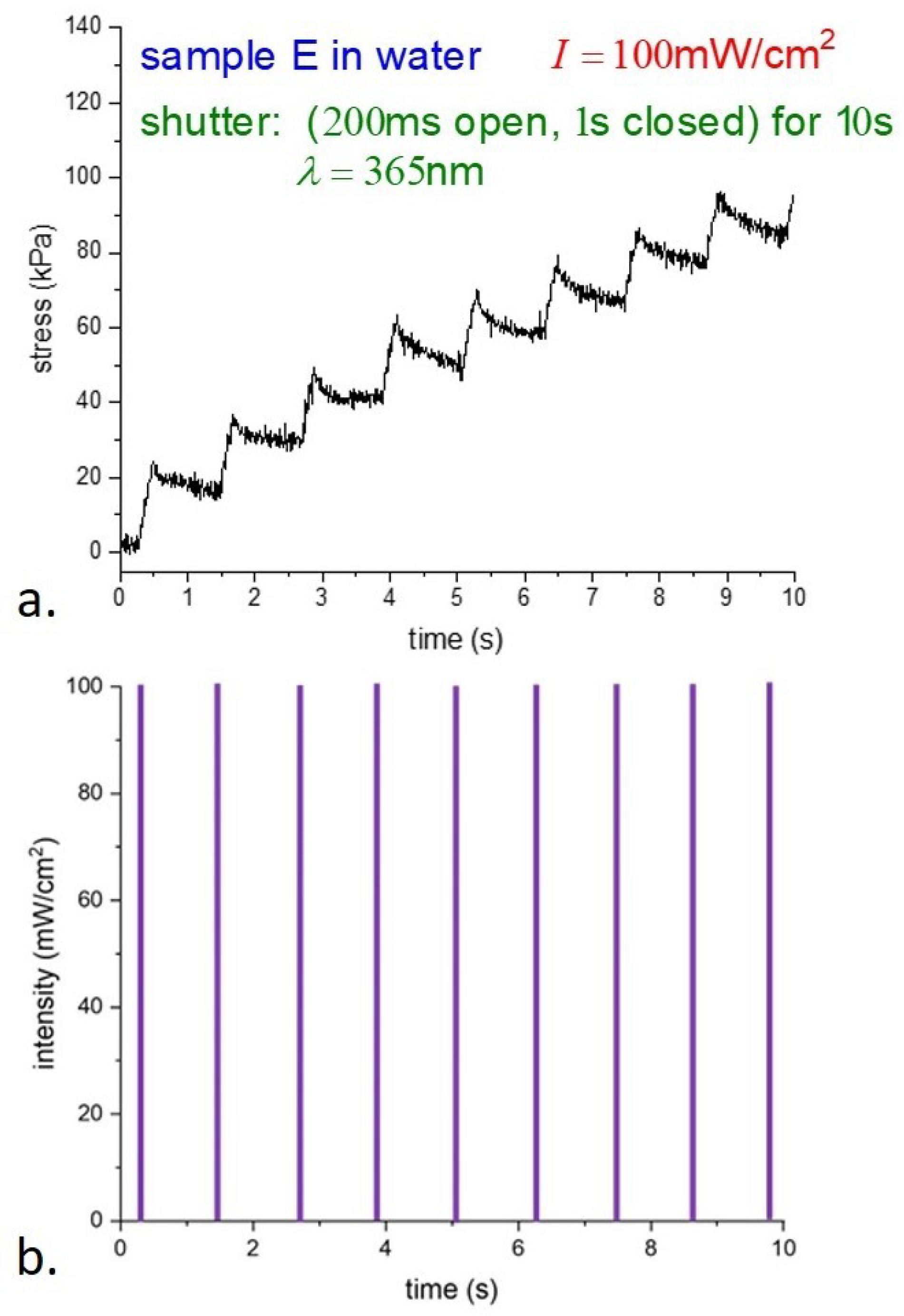
Although the data were collected at different times and on different time scales, the behavior of samples K and E was found to be essentially similar throughout. To avoid unnecessary duplication, we focus on the response of E-type samples below. Samples were suspended underwater in a thin-walled glass container and photostress measurements were taken with pulsed illumination as before. Stress underwater versus time for two different illumination intensities is shown in Figure 6.

As shown in Figure 6, the response of samples illuminated at different intensities saturates at very nearly the same stress, while the intensities differ by a factor of $2.5$. The time to reach the photostationary state, where essentially all the dye molecules are in the cis-state, is, in dimensional units from theory, is $t = \tau /(I/I_0) = 2.5$ s if $I = 40$ mW/cm², and $t = 1$ s for $I = 100$ mW/cm². The experiment from Figure 6a gives 7 s, and from Figure 6b gives 3 s, which are in good agreement with the theory.

Expanding the time scale and showing the leading edge of the light pulses, Figure 7 shows a rapid increase in the photostress with light, then a slow decay to a steady value. The details of the relaxation are not clear; we anticipate a possible connection with the results of [26].

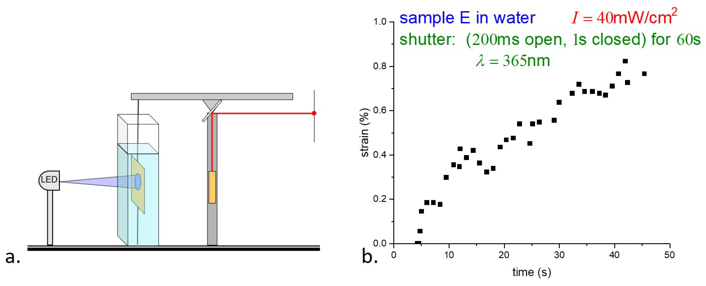
4.2. Photostrain

The photostrain of the samples was measured using a modified version of the apparatus shown in Figure 4. As shown in Figure 8a, a horizontal light beam on two point supports was mounted on top of the vertical post to act as a beam balance. An E-type sample was held as before, with the bottom edge attached to the table and the top edge to the balance beam. The length of the filament was adjusted so that the balance beam was nearly horizontal and the tension in the filament was nearly zero. The beam of a small HeNe laser, mounted on a vertical post, was reflected by a mirror attached to the balance beam at its fulcrum. A contraction of the sample causes rotation of the beam and mirror, and the displacement of the reflected laser spot in the far field enables the determination of the sample strain. Again, the sample was held underwater to minimize sample heating by the UV light. Although illumination was the same as for the stress measurements underwater (200 ms illumination followed by 1 s darkness), the uncertainty in the strain measurements is much greater than in the stress measurements. (A $0.1\%$ strain requires a challenging 20 $\mathsf{\mu }$m displacement resolution.) Although the balance beam is light and well balanced, its response time, due to its moment of inertia, leads to averaging the response. Although the accuracy is far from ideal, the photostrain measurements in Figure 8b nonetheless appear consistent with the saturation of the photostress of ∼45 s in Figure 6a.

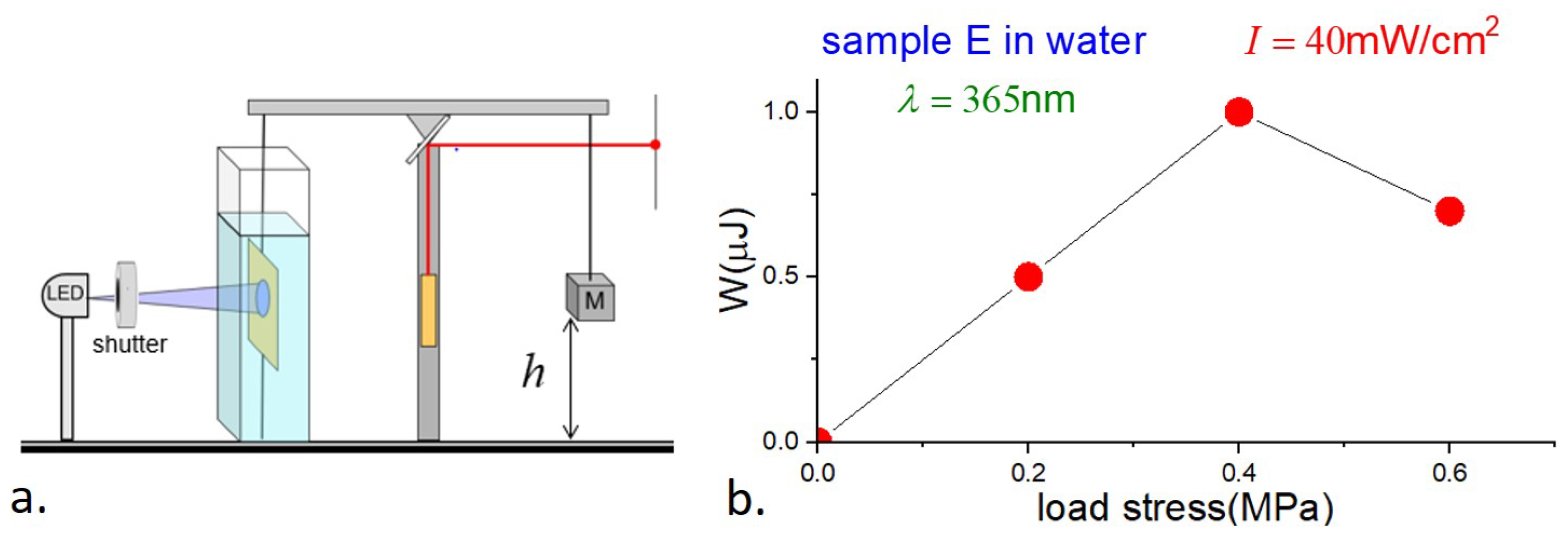
4.3. Photowork

Our final measurements involved the determination of photowork and light-to-work efficiency by E-type samples. The balance beam was balanced as in the strain measurements; a load was then applied by suspending a known mass near the other end of the balance beam, and the sample was illuminated with continuous UV at 365 nm and 40 mW/cm² intensity. The position of the laser spot in the far field provided information about the change in the height of the load as a function of time. A schematic is shown in Figure 9a.

The results, showing the loads F, displacements $\Delta h$, and work W, are presented in

Table 3. Data for photowork and efficiency.

M (kg)	F (N)	$\mathit{\sigma }$ (Pa)	$\mathbf{\Delta }\mathit{h}$ (m)	W (J)	$\mathbf{\Gamma }$
0	0	0	$3.1\times {10}^{-5}$	0	0
$1\times {10}^{-3}$	$1\times {10}^{-2}$	$2\times {10}^5$	$4.9\times {10}^{-5}$	$5\times {10}^{-7}$	$2\times {10}^{-5}$
$2\times {10}^{-3}$	$2\times {10}^{-2}$	$4\times {10}^5$	$5.5\times {10}^{-5}$	$10\times {10}^{-7}$	$5\times {10}^{-5}$
$3\times {10}^{-3}$	$2\times {10}^{-2}$	$6\times {10}^5$	$2.4\times {10}^{-5}$	$7\times {10}^{-7}$	$3\times {10}^{-5}$

, together with the efficiency $\mathrm{\Gamma }$, which is the photomechanical work done divided by the energy of the absorbed light,

$$\mathrm{\Gamma }=\frac{F\Delta h}{{\rho }_{0}h\nu V},$$

(26)

where V is the sample volume. The uncertainties in the strain, and hence in the work and efficiency, are estimated to be ∼10%.

We have no ready explanation for the curious observation that the photostrain with load is greater than without. There are at least two possible contributing factors. First, in our photostrain measurements, the sample was held vertically, but no additional tension was applied, and the sample may not have been perfectly planar. Second, the stress on the sample due to the load gave rise to tensile stress (magnitude comparable to $1\%$ of the modulus), which may have increased the orientational order and hence photostrain in the sample.

5. Summary

In this work, we proposed a precise definition of the critical intensity $I_0$, a material parameter that sets the scale of energy flux for photoactuation. To determine the value of $I_0$ for extensively studied azo-acrylate materials, we needed the values of the cis-isomer relaxation time and the absorption cross-section of the trans-isomer. From the dynamic absorption spectrum measurements, we determined that the cis-relaxation time of our samples is ∼10⁴ s. From the absorption measurements, we determined that the absorption cross-section of the trans-isomer at 365 nm is ${10}^{-21}$ m². Based on these, we showed that the critical intensity is $I_0 = {10}^{-2}$ mW/cm². This value is remarkably low; typical photomechanical measurements use intensities of 100 mW/cm², giving the ratio $I/I_0 = {10}^4$. We then considered the dependence of the system response on the ratio $I/I_0$. We identified three distinct regimes and we discussed their characteristics. In regime 3, corresponding to typical excitation intensities, the response time is ∼1 s, and on this timescale, the response is fluence dependent. Once the system saturates, no further absorption takes place, and the cis-isomer density and the bulk photostress remains constant at zero strain. We anticipate future experiments to further verify and utilize our results.