Multiple-Image Reconstruction of a Fast Periodic Moving/State-Changed Object Based on Compressive Ghost Imaging

Abstract

We propose a multiple-image reconstruction scheme of a fast periodic moving/state-changed object with a slow bucket detector based on compressive ghost imaging, named MIPO-CSGI. To obtain N frames of an object with fast periodic moving/state-changed, N random speckle patterns are generated in each cycle of the object, which are then used to illuminate the object one by one. The total energy reflected from the object is recorded by a slow bucket detector at each cycle time T. Each group with N random speckle patterns is programmed as one row of a random matrix, and each row of the matrix element corresponds to one measurement of the slow bucket detector. Finally, the compressive sensing algorithm is applied to the constructed matrix and bucket detector signals, resulting in the direct acquisition of multiple images of the object. The feasibility of our method has been demonstrated in both numerical simulations and experiments. Hence, even with a slow bucket detector, MIPO-CSGI can image a fast periodic moving/state-changed object effectively.

1. Introduction

Ghost imaging (GI), also known as correlated imaging (CI), has been extensively researched as a novel imaging method in recent years [1,2,3,4,5]. GI acquires object information by utilizing two spatially correlated optical beams. One beam known as the object beam crosses an object, and the reflected (or transmitted) signal is detected by a single-pixel bucket detector. The other beam, known as the reference beam, never interacts with the object and is detected by a spatially resolving detector. By calculating the correlation between the two beams, the image of the object can be recovered, and neither of them can restore the image of the object alone [6,7]. The demonstration of GI using entangled photons was explained as a quantum phenomenon firstly [8,9]. Subsequently, pseudothermal light sources and thermal light sources used in GI have also been proven effective [10,11,12]. Then, as a variant of the standard two-detector pseudothermal GI, computational ghost imaging (CGI), which simplifies the double optical paths to a single optical path and precomputes the reference patterns, further enhances the application of GI [13,14,15,16].

Recently, several papers have been devoted to studying GI in imaging moving objects. The condition of GI to imaging a moving object was firstly given by the second-order correlation function through quasistatic approximation [17]. Later, it was proven that Fourier-transform ghost diffraction has the ability to overcome the influence of the system’s shaking [18]. Then, the methods to overcome the decline of GI resolution caused by the tangential or axial movement of moving objects relative to the imaging system were discussed [19,20]. Meanwhile, background-subtracted images of moving targets were reconstructed by using compressive sensing (CS) and complementary modulation techniques [21]. By tracking the target position or motion trajectory captured by the under-sampled image, the moving object’s deblurred image can be gradually obtained [22,23]. With the prior knowledge of the motion, a method of setting the object as static and inversely transforming the illumination mode to image a moving object was proposed [24]. To compensate for the limited rate of structured illumination, structured illumination based on the light-emitting diode (LED) was designed to capture images of moving objects [25,26]. As CGI requires a certain number of measurements in one image, to reconstruct the image of a moving object with high quality, the object is always assumed to be relatively static during the measurement period. From the above works, we can see that there are two ways to improve the performance of imaging the moving object in CGI. One method is to design an optimization algorithm to reduce the number of measurements during the relative static period of the object as much as possible. Another way is to improve the performance of the devices in CGI to produce more speckle patterns and enable more detection in a small period. However, these schemes all need a high sampling bucket detector that performs the detection of the relatively static object in each measurement. In our previous work, we proposed a new scheme that uses a slow bucket detector to image an object with fast periodic moving/state-changed [27]. However, more speckle patterns and measurement times are required, resulting in an excessively long sampling time.

Since traditional GI uses random speckle patterns, the number of measurements required to obtain a good reconstruction of an N-pixel image is much greater than N [28]. Subsequently, compressive ghost imaging (CSGI) was proposed to obtain better imaging performance from fewer than N measurements by exploiting the sparsity of the object, at the expense of computational time for the reconstruction [29,30].

In this paper, we propose a method that uses a slow bucket detector to image objects with fast periodic moving/state-changes based on CSGI, and we call it MIPO-CSGI. In MIPO-CSGI, when we want to obtain the N frames of a fast periodic moving/state-changed object, we modulate N random speckle patterns in each cycle T of the object (the object has a known cycle time T). Then, using N speckle patterns as a group, we illuminate the periodic moving/state-changed object and collect the total intensity value reflected from the object as one measurement through a slow bucket detector at each cycle time T. We program each group of the speckle patterns as one row of a random matrix. As the object moves or changes periodically, we will obtain a series of bucket detector values and one random matrix. Finally, N frames of the object can be obtained directly by applying the compressive sensing algorithm to the bucket detector signals and the programmed random matrix. The advantage of this scheme is that even if the slow bucket detector is used, any number of high-quality frames of fast periodic moving/state-changed objects can be captured with fewer measurements.

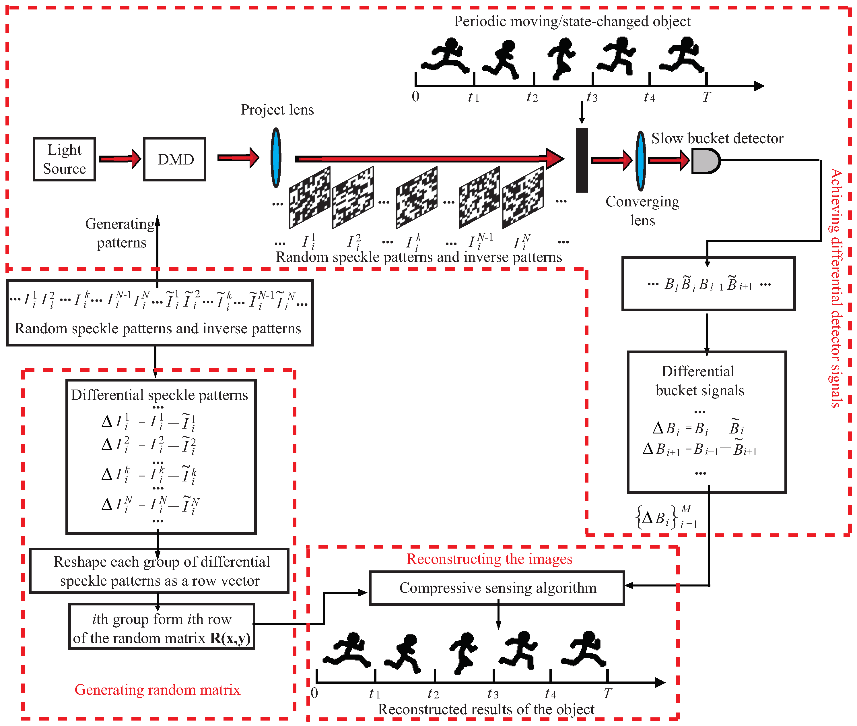
2. Theory and Methods

The MIPO-CSGI schematic diagram is illustrated in Figure 1, which has a part to achieve differential detector signals, a part to generate a random matrix, and a part to reconstruct the images. In the achieving differential detector signals part, the light field is modulated by a digital micro-mirror device (DMD) to produce pairs of random speckle patterns. Each speckle pattern pair includes a speckle pattern $I_i^k(x,y)$ and its inverse pattern ${\tilde{I}}_i^k(x,y)$, where, $x=1,2,\cdots ,N_x$, $y=1,2,\cdots ,N_y$, i is the ith number of the groups, k represents the kth number of the speckle patterns in each group, and the speckle patterns are either white 1 or black −1 for each coordinate (x,y). According to the differential acquisition method [21,31], we set $I_i^k(x,y)=-{\tilde{I}}_i^k(x,y)$.

In traditional CGI, the sampling rate of the bucket detector is high or equal to the frequency of the state switching of the object. When a slow bucket detector is used to obtain N frames of the periodic moving/state-changed object, we need to produce N random speckle patterns $I_i^k(x,y),k=1,2,\cdots ,N$ as one group according to the cycle time T of the object and use them to illuminate the object ${\left\{T(x,y,k)\right\}}_{k=1}^N$, which is then measured by the slow bucket detector and recorded as $B_i$:

$$B_i=\eta \int \int \int I_i^k(x,y)T(x,y,k)dxdydk+n,$$

(1)

where $\eta$ is the bucket detector’s responsivity, and n is the noise generated by environmental illuminations. Similarly, corresponding to ${\tilde{I}}_i^k(x,y),k=1,2,\cdots ,N$, we can obtain the detection result ${\tilde{B}}_i$ expressed as:

$${\tilde{B}}_i=\eta \int \int \int {\tilde{I}}_i^k(x,y)T(x,y,k)dxdydk+n.$$

(2)

Thus, the differential detector signal $▵B_i$ between the two corresponding detection results $B_i$ and ${\tilde{B}}_i$ can be expressed as:

$$\begin{array}{cc}\hfill ▵B_i& =B_i-{\tilde{B}}_i\hfill \\ \hfill & =\eta \int \int \int (I_i^k(x,y)-{\tilde{I}}_i^k(x,y))T(x,y,k)dxdydk\hfill \\ \hfill & =\eta \int \int \int ▵I_i^k(x,y)T(x,y,k)dxdydk,\hfill \end{array}$$

(3)

where $▵I_i^k(x,y)=I_i^k(x,y)-{\tilde{I}}_i^k(x,y)$. It can be seen that the environmental noise can be efficiently removed.

With M measurements, we will obtain M groups of random speckle patterns ${\left\{I_i^k(x,y)\right\}}_{i=1}^M$ $(k=1,2,\cdots ,N)$ and their corresponding bucket detector signals ${\left\{B_i\right\}}_{i=1}^M$. Meanwhile, M groups’ inverse patterns ${\left\{{\tilde{I}}_i^k(x,y)\right\}}_{i=1}^M$$(k=1,2,\cdots ,N)$ also correspond to M bucket detector signals ${\left\{{\tilde{B}}_i\right\}}_{i=1}^M$ and will be obtained by other M measurements. Therefore, we will obtain M groups of differential speckle patterns ${\{▵I_i^k(x,y)\}}_{i=1}^M(k=1,2,\cdots ,N)$ and their corresponding differential bucket detector signals ${\{▵B_i\}}_{i=1}^M$.

In the generating random matrix part, each speckle pattern $▵I_i^k(x,y)$ can be reshaped as a row vector ${\mathbf{I}}_i^k$ with size $1\times K$, where $K=N_x\times N_y$:

$$\begin{array}{c}\hfill \begin{array}{cc}\hfill {\mathbf{I}}_i^k& =[▵I_i^k(1,1)\cdots ▵I_i^k(1,N_y)▵I_i^k(2,1)\cdots \hfill \\ \hfill & ▵I_i^k(2,N_y)\cdots ▵I_i^k(N_x,1)\cdots ▵I_i^k(N_x,N_y)].\hfill \end{array}\end{array}$$

(4)

Each group with N speckle patterns $▵I_i^k(x,y)$$(k=1,2,\cdots ,N)$ can form a row vector ${\mathbf{A}}_i$, with size $1\times P$, where $P=N\times K$:

$$\begin{array}{c}\hfill \begin{array}{cc}\hfill {\mathbf{A}}_i& =[{\mathbf{I}}_i^1{\mathbf{I}}_i^2\cdots {\mathbf{I}}_i^N]\hfill \\ \hfill & =[▵I_i^1(1,1)\cdots ▵I_i^1(N_x,N_y)▵I_i^2(1,1)\cdots \hfill \\ \hfill & ▵I_i^2(N_x,N_y)\cdots ▵I_i^N(1,1)\cdots ▵I_i^N(N_x,N_y)].\hfill \end{array}\end{array}$$

(5)

M groups’ differential speckle patterns ${\{▵I_i^k(x,y)\}}_{i=1}^M(k=1,2,\cdots ,N)$ can construct an $M\times P$ matrix $\mathbf{R}$ as:

$$\begin{array}{c}\hfill \begin{array}{cc}\hfill \mathbf{R}& =\left[\begin{array}{c}{\mathbf{A}}_1\\ {\mathbf{A}}_2\\ ⋮\\ {\mathbf{A}}_M\end{array}\right]\hfill \\ \hfill & =\left[\begin{array}{cccc}▵I_1^1(1,1)& ▵I_1^1(1,2)& \cdots & ▵I_1^N(N_x,N_y)\\ ▵I_2^1(1,1)& ▵I_2^1(1,2)& \cdots & ▵I_2^N(N_x,N_y)\\ ⋮& ⋮& \ddots & ⋮\\ ▵I_M^1(1,1)& ▵I_M^1(1,2)& \cdots & ▵I_M^N(N_x,N_y)\end{array}\right].\hfill \end{array}\end{array}$$

(6)

Equation (3) can be expressed in a matrix form:

$$\begin{array}{c}\hfill \begin{array}{cc}\hfill \left[\begin{array}{c}▵B_1\\ ▵B_2\\ ⋮\\ ▵B_M\end{array}\right]& =\eta \left[\begin{array}{cccc}▵I_1^1(1,1)& ▵I_1^1(1,2)& \cdots & ▵I_1^N(N_x,N_y)\\ ▵I_2^1(1,1)& ▵I_2^1(1,2)& \cdots & ▵I_2^N(N_x,N_y)\\ ⋮& ⋮& \ddots & ⋮\\ ▵I_M^1(1,1)& ▵I_M^1(1,2)& \cdots & ▵I_M^N(N_x,N_y)\end{array}\right]\left[\begin{array}{c}T(1,1,1)\\ T(1,2,1)\\ ⋮\\ T(N_x,N_y,N)\end{array}\right],\hfill \end{array}\end{array}$$

(7)

where ${\mathbf{T}}_N={\left[T(1,1,1)T(1,2,1)\cdots T(N_x,N_y,N)\right]}^T$ is a $P\times 1$ column vector representing the object’s transmission coefficient ${\left\{T(x,y,k)\right\}}_{k=1}^N$.

In reconstructing the images part, to reduce the number of measurements, the CS algorithm is used to reconstruct ${\left\{T(x,y,k)\right\}}_{k=1}^N$. Here, we use the TVAL3 algorithm [32], which has the advantage of reconstructing high-quality images with fewer measurements. Therefore, the object’s N images ${\left\{\widehat{T}(x,y,k)\right\}}_{k=1}^N$ can be reconstructed by:

$$\begin{array}{c}\hfill \begin{array}{c}\hfill \min \sum _j\parallel D_j{\mathbf{T}}_N{\parallel }_1+\frac{\mu }{2}{\parallel \mathbf{B}-\mathbf{R}{\mathbf{T}}_N\parallel }_2^2,\end{array}\end{array}$$

(8)

where $\mathbf{B}$ is a $M\times 1$ column vector consisting of the M differential bucket detector signals ${\{▵B_i\}}_{i=1}^M$. $D_j{\mathbf{T}}_N$ denotes the discrete gradient of ${\mathbf{T}}_N$ at element $j(j=1,2,\cdots ,P)$, ${\sum }_j\parallel D_j{\mathbf{T}}_N\parallel$ is the discrete total variation of ${\mathbf{T}}_N$, ${\parallel ·\parallel }_1$ and ${\parallel ·\parallel }_2$ stand for the $l_1$ norm and $l_2$ norm, respectively, $\mu$ is a coefficient used to balance data fidelity and regularization, and here we set $\mu$ equal $2^{12}$.

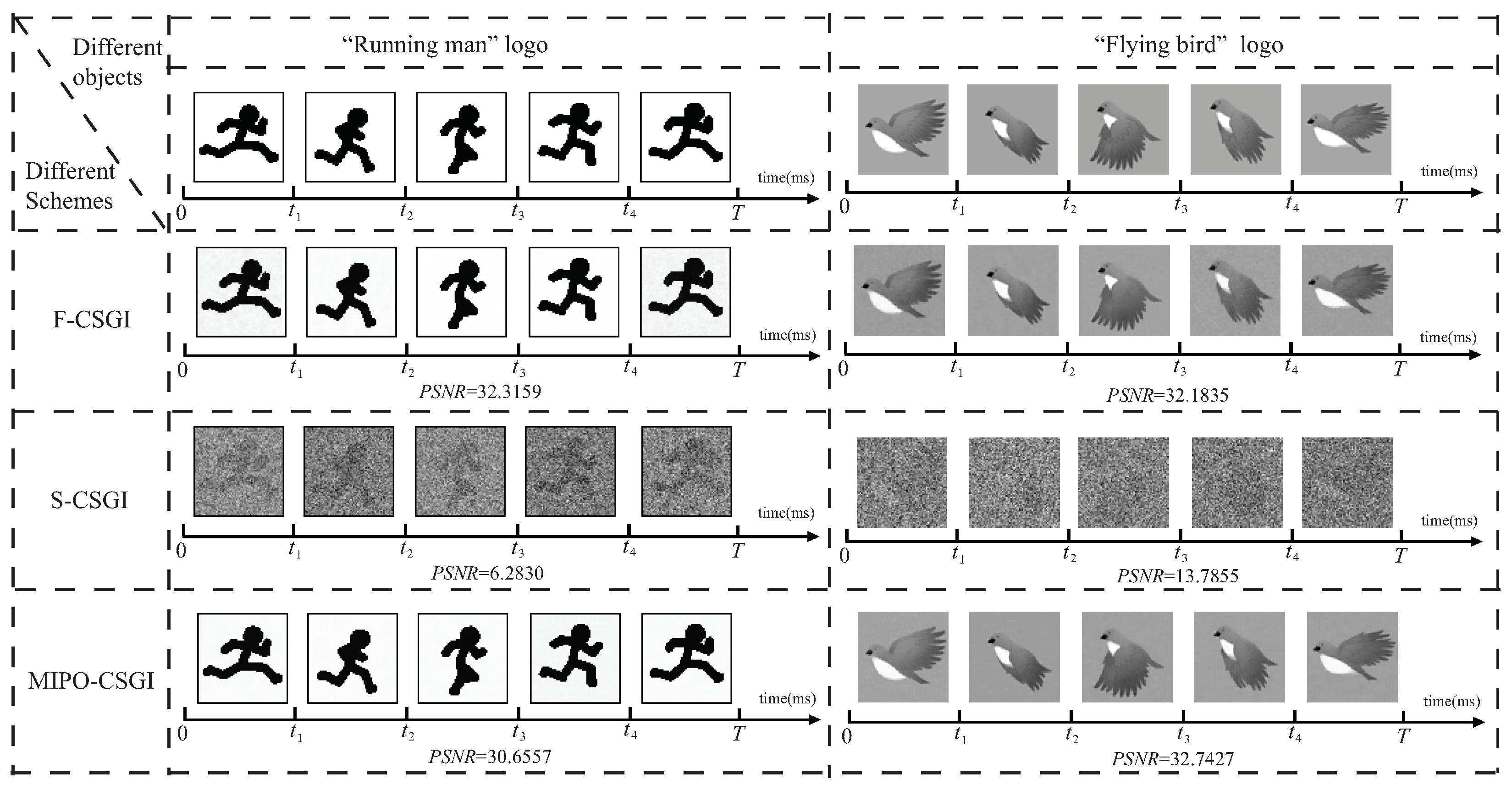
3. Numerical Verification

In this section, numerical simulations are used to validate the effectiveness of MIPO-CSGI. The image resolution of each target is set to 64 × 64. The simulations are carried out on Matlab R2018a on the Windows 11 operating system. The hardware system is a laptop with a 3.20 GHz central processor unit (AMD Ryzen 7 5800H) and 16.0 GB of random access memory. Additionally, we use the peak signal-to-noise ratio (PSNR) as an objective evaluation, as defined by the following definition [29,33]:

$$\begin{array}{c}\hfill \begin{array}{c}\hfill PSNR=10lo{g}_{10}\left[\frac{{255}^2}{\frac{1}{N_x·N_y}{\sum }_{x,y}{(\widehat{T}(x,y)-T(x,y))}^2}\right],\end{array}\end{array}$$

(9)

where $T(x,y)$ and $\widehat{T}(x,y)$ are the original and recovered image intensity values, respectively. $N_x$ and $N_y$ represent the object’s horizontal and vertical dimensions. In general, the higher the PSNR value, the higher the quality of the reconstructed image. Meanwhile, we characterize the compressive sampling ratio by the parameter $\beta =M/P$, which is defined as a ratio of the number of measurements M to the total pixels P of the multiple images.

We first perform numerical simulations by imaging the periodic moving object to verify the feasibility of MIPO-CSGI. The MIPO-CSGI reconstruction results are compared to those of CSGI using a fast bucket detector (F-CSGI) and CSGI using a slow bucket detector (S-CSGI). In F-CSGI, the sampling rate of the fast bucket detector is high or equal to the frequency of the state switching of the object, and each bucket detector value corresponds to one speckle pattern acting on each state of the object. The sampling rate of the slow bucket detectors in S-CSGI and MIPO-CSGI is slower, so they can only record the total energy of each group of the speckle patterns acting on the object at each cycle time T. Assume the original objects are two two-grayscale objects such as a jumping “square”, a moving “T”, and an eight-grayscale moving “spacecraft”. Taking the jumping “square” as an example, in order to obtain four frames of the object, we use the computer to simulate DMD to produce four 64 × 64-resolution random speckle patterns in each cycle. The sampling rate of the bucket detector used in F-CSGI is four times that in MIPO-CSGI and S-CSGI, which also means that to get the same number of the bucket detector signals, the number of speckle patterns and the optical measurements time in MIPO-CSGI and S-CSGI is four times that of F-CSGI. Then, one by one, each speckle pattern is used to illuminate each state of the periodic moving object. When $\beta$ is set to 60.01%, each scheme will obtain 9,832 differential bucket detector signals. We will obtain a 9832 × 16,384-resolution random matrix in MIPO-CSGI. As the reconstruction results are shown in Figure 2, four frames of the “square” reconstructed by MIPO-CSGI and F-CSGI both have a high PSNR. Because the fast bucket detector is fast at making enough measurements of each state of the moving object, F-CSGI can reconstruct the images of the object with high quality. Although the slow bucket detector cannot capture each state of the moving object, MIPO-CSGI programmed a random matrix, constructed from four speckle patterns used in each cycle time T. MIPO-CSGI makes the total energy value detected by the slow bucket detector in one cycle time T equivalent to one measurement of the effect of a large speckle pattern composed of a row of the constructed matrix on a large static image composed of each state of a moving object. With a certain amount of measurements, MIPO-CSGI can also reconstruct a large image with each state of the object of high quality. Although the PSNR of F-CSGI is almost the same as the MIPO-CSGI, the sampling rate of the bucket detector in F-CSGI is four times that in MIPO-CSGI. For S-CSGI, each detector value of the slow detector of each cycle T is equivalent to one state of the object detected by the bucket detector, and noise composed of other state detections is added. So, with the same slow bucket detector, the PSNR value of MIPO-CSGI is better than that of S-CSGI. For the moving “T”, we just need to perform the same operation as imaging the jumping “square”. From Figure 2, we can see that MIPO-CSGI reconstructs four frames of the “T”, as well as the jumping “square”. We can also image each state of the moving “spacecraft”, although its operation trajectory is more complex. The reconstruction results of the “spacecraft” further confirm the MIPO-CSGI’s effectiveness.

To further compare the performance of F-CSGI, S-CSGI, and MIPO-CSGI, we take the jumping “square” as the target to simulate these schemes with varying compressive sampling ratios $\beta$. Due to the randomness of the reconstruction results of random speckle patterns in CGI, we present the average PSNR values of the reconstructed images using F-CSGI, S-CSGI, and MIPO-CSGI schemes at 10 times. The results are presented in Figure 3. From Figure 3, it can be seen that the PSNR of S-CSGI under different compression rates $\beta$ is almost unchanged. The PSNRs of F-CSGI and MIPO-CSGI under different compressive sampling ratios $\beta$ are almost the same, and both increase with the increase in the compressive sampling ratios. Under the same imaging quality, the sampling rate of the bucket detector in F-CSGI is four times that of MIPO-CSGI, and the PSNR of MIPO-CSGI is significantly higher than that of S-CSGI under the same sampling rate of the bucket detector.

In addition, numerical simulations for the periodic state-changed object with MIPO-CSGI, F-CSGI, and S-CSGI are performed in Figure 4. The original objects are 64 × 64-resolution two-grayscale “running man” and 64 × 64-resolution eight-grayscale “flying bird”. Taking the “running man” as an example, five 64 × 64-resolution random speckle patterns with their inverse speckle patterns are modulated in each cycle to obtain five frames of the object. Meanwhile, the bucket detector’s sampling rate in F-CSGI is five times that in MIPO-CSGI, and the bucket detector’s sampling rate in MIPO-CSGI is the same as that in S-CSGI. With a 60.01% compressive sampling ratio, all schemes will obtain 12,290 differential bucket detector signals. One 12,290 × 20,480-resolution random matrix will be programmed in MIPO-CSGI. Figure 4 shows that the PSNR of MIPO-CSGI is almost the same as that of F-CSGI and more than twice that of S-CSGI. According to the reconstruction result of MIPO-CSGI and F-CSGI, we can easily obtain the motion state of the object. The reconstructed “flying bird” also verifies that MIPO-CSGI can image eight-grayscale objects with fast periodic state-changes, which further proves the effectiveness of MIPO-CSGI.

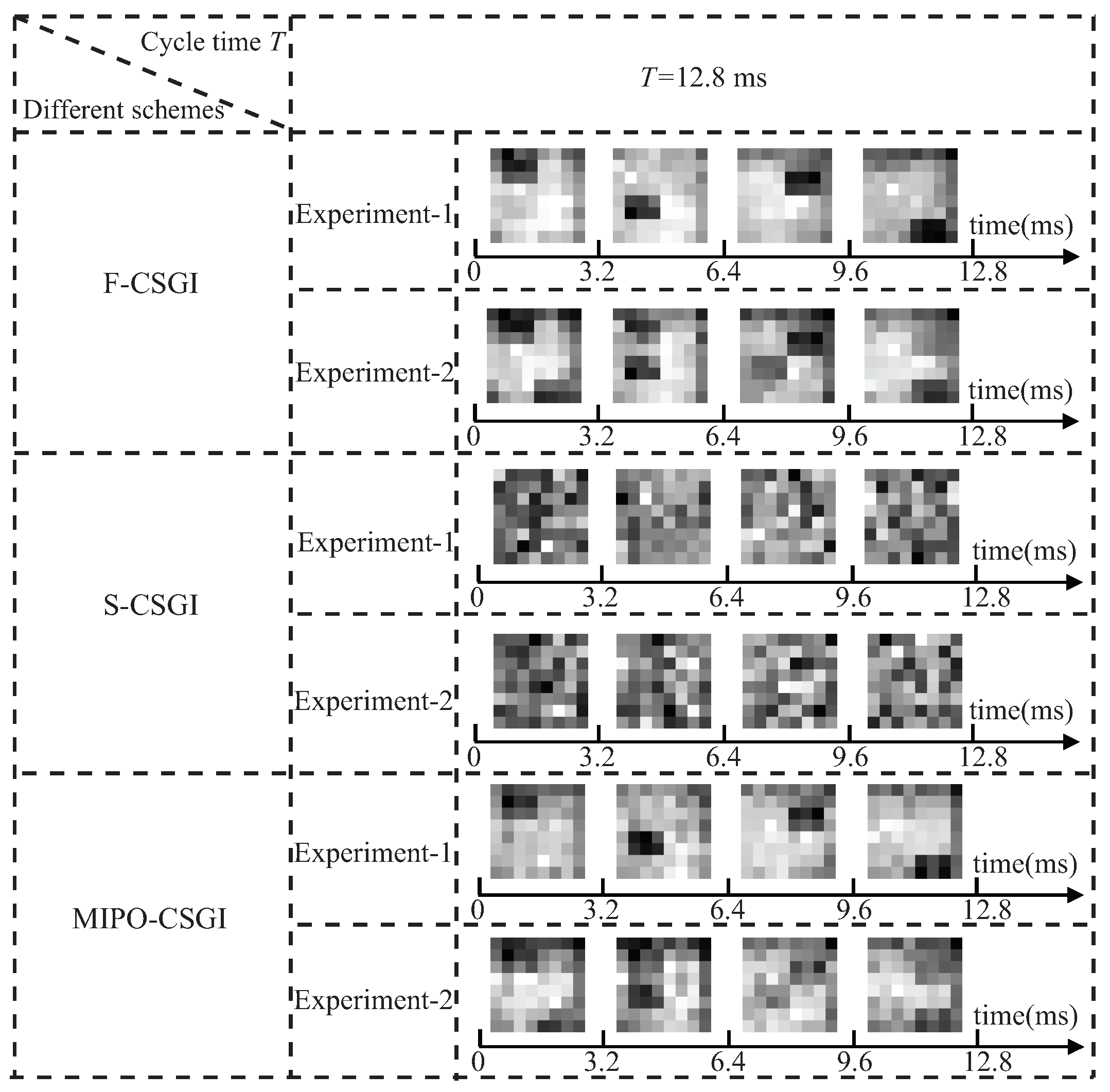
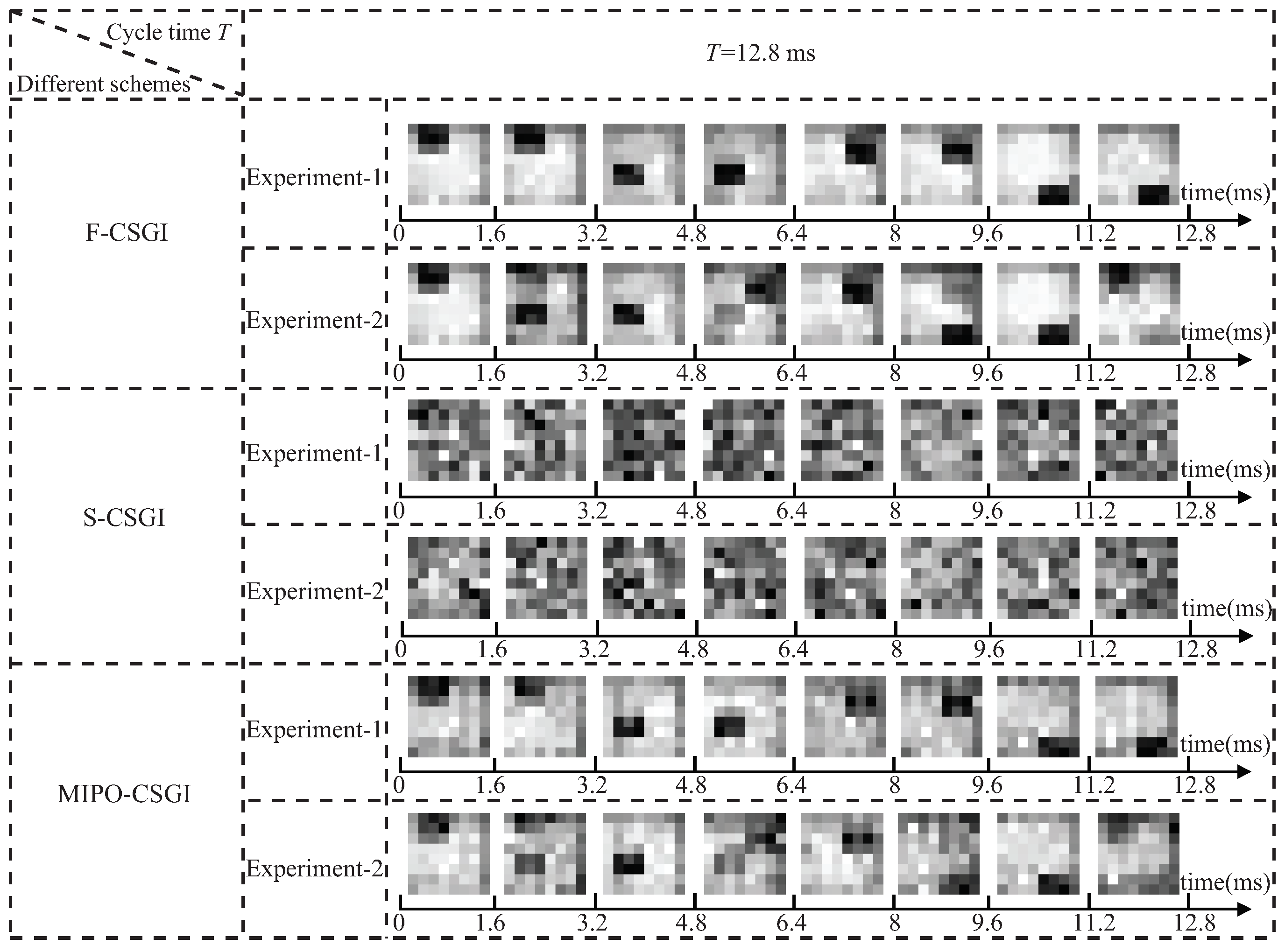
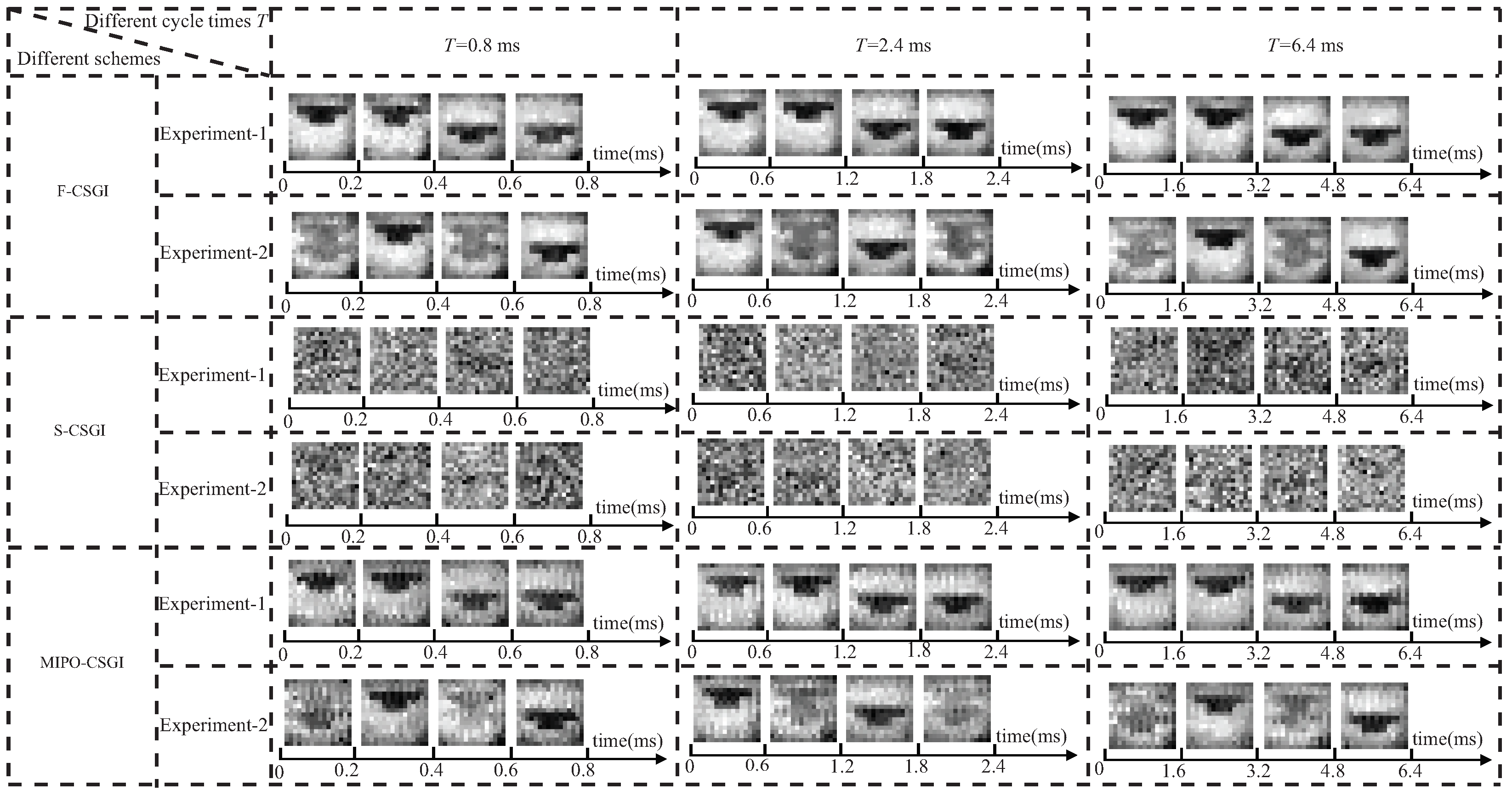
4. Experimental Verification

Next, MIPO-CSGI is verified experimentally. The experimental setup of MIPO-CSGI is shown in Figure 5. Computer-1 controls DMD-1 (TI DLPC350), modulates the light emitted by an LED, and generates a series of speckle patterns pairs, $I_i^k(x,y)$ and ${\tilde{I}}_i^k(x,y)$. Then, a projector lens projects the speckle patterns onto DMD-2 (TI DLPC350). Computer-2 controls DMD-2 to repeatedly display the object with a cycle time T. A lens (focal length is 50 mm) collects the light reflected from the object, which is detected by a slow bucket detector (Thorlabs PDA100A2), and the paired detection results $B_i$ and ${\tilde{B}}_i$ are generated in turn. With the operation repeated $2\times M$ times, we will obtain M differential signals ${\{▵B_i\}}_{i=1}^M$ by $B_i-{\tilde{B}}_i(i=1,2,\dots ,M)$. Meanwhile, computer-1 will program matrix $\mathbf{R}$ based on the M groups’ differential speckle patterns ${\{▵I_i^k(x,y)\}}_{i=1}^M(k=1,2,\cdots ,N)$. Finally, we use the compressive sensing algorithm to obtain multiple images of the target based on matrix $\mathbf{R}$ and ${\{▵B_i\}}_{i=1}^M$ generated by computer-1.

Four frames of the jumping “square” chosen from Figure 2 are selected as the experimental target to validate MIPO-CSGI’s reconstruction ability. In the experiment, DMD-2 displays four frames of 1024 × 768-resolution jumping “square” with a cycle time T of 12.8 ms. Then, each random speckle pattern is modulated by DMD-1 to 8 × 8-resolution. We set four speckle patterns in each cycle to obtain four frames of the object. The compressive sampling ratio of MIPO-CSGI, F-CSGI, and S-CSGI is set up to 70.31%, which means there will be 180 differential bucket detector signals obtained in each scheme. We will program a 180 × 256-resolution random matrix in MIPO-CSGI, and the sampling rate of the bucket detector in F-CSGI will be four times that of MIPO-CSGI and S-CSGI. Meanwhile, the total optical measurement time used in MIPO-CSGI and S-CSGI is four times that in F-CSGI. Figure 6 shows the results of two sets of experiments using MIPO-CSGI, F-CSGI, and S-CSGI. The experimental results-1 of MIPO-CSGI, F-CSGI, and S-CSGI are similar to the simulation results in Figure 2. Because the detection results are inevitably influenced by background and detector noise, even when the compression ratio is high, the reconstructed image quality of the experimental results in Figure 6 will be lower than the numerical simulation results in Figure 2. The bucket detector has a slow sampling rate and a long sampling time, which means that more environmental noise is introduced. Therefore, there is a certain attenuation in the imaging quality of MIPO-CSGI compared with F-CSGI in the experiment. It is known that DMD requires a certain amount of time to refresh and display different objects. During the experiment, we may obtain the intermediate states displayed by the DMD-2 switching between two frames, as shown in experimental results-2. As illustrated in Figure 6, although F-CSGI has a better reconstruction ability than MIPO-CSGI, it is hard to obtain information about the object when a slow bucket detector is used in S-CSGI. To obtain eight frames of the object, eight $8\times 8$-resolution speckle patterns with their inverse speckle patterns are generated in each cycle time T. With a 70.31% compressive sampling ratio, a 360 × 512-resolution random matrix will be recorded by computer-1 in MIPO-CSGI. All of these schemes will record 360 differential bucket detector signals. Meanwhile, the bucket detector’s sampling rate in F-CSGI is set to be eight times that in MIPO-CSGI and S-CSGI. As can be seen from Figure 7, we can see that F-CSGI and MIPO-CSGI will produce eight frames of the object as experimental results-1 or produce four frames and four intermediate states of the object as experimental results-2. S-CSGI still cannot obtain any information about the jumping “square”.

The experiments are then carried out on different cycle times T of the two middle frames “T” chosen from Figure 2 to investigate the effectiveness of MIPO-CSGI. DMD-2 displays two frames of the moving “T” at 1,024 × 768-resolution under different cycle times T as 0.8 ms, 2.4 ms, and 6.4 ms, respectively. Here, each random speckle pattern is modulated by DMD-1 to 16 × 16-resolution. To obtain two frames of the “T”, we must modulate two 16 × 16-resolution speckle patterns in each cycle time T. With $\beta$ set to 69.92%, we will obtain a 358 × 512-resolution random matrix in MIPO-CSGI, and the bucket detector’s sampling rate in F-CSGI is set to twice that in MIPO-CSGI and S-CSGI. Figure 8 depicts the experimental results of MIPO-CSGI, F-CSGI, and S-CSGI. Both MIPO-CSGI and F-CSGI can image the object “T” into two frames as experimental results-1 or two intermediate states as experimental results-2. The longer the cycle time T of the object, that is, the longer the DMD-2 displays each state of the moving object, as shown in Figure 8, the better the imaging quality of MIPO-CSGI. We cannot obtain the motion information of the moving “T” from the reconstruction results of S-CSGI. Furthermore, we compare the experimental results of MIPO-CSGI, F-CSGI, and S-CSGI for obtaining four frames of the “T” under different cycle times T as 0.8 ms, 2.4 ms, and 6.4 ms, respectively. Figure 9 shows that both MIPO-CSGI and F-CSGI can image the “T” into four frames, as in experimental result-1, or into two frames and two intermediate states, as in experimental result-2. Due to the use of a slow bucket detector, S-CSGI is consistently unable to image moving objects. Therefore, the effectiveness of the MIPO-CSGI is further validated.

5. Conclusions

In conclusion, we have proposed MIPO-CSGI, which employs a slow bucket detector to image a fast periodically moving/state-changed object using compressive ghost imaging. The proposed scheme constructed a random matrix based on the speckle patterns which acted on the object in each cycle T and establish a one-to-one correspondence between each row of the matrix and the measurement of the slow bucket detector. The multi-frame imaging of a periodically moving/state-changed object is converted into the imaging of a static large image composed of each state of the moving object to compensate for the sampling rate of the bucket detector. Finally, compressive sensing is used to reconstruct multiple images based on the random matrix with fewer bucket detector measurements. To further prove the feasibility of MIPO-CSGI, simulations and experiments are taken to compare with traditional F-CSGI, which uses a fast bucket detector, and S-CSGI, which uses a slow bucket detector. Through the simulations, we can see the imaging quality of MIPO-CSGI is almost the same as that of F-CSGI and better than that of S-CSGI. In the experiments, the noise introduced by the long response time of the slow detector makes the imaging quality of MPIO-CSGI slightly lower than that of F-CSGI, but it is always better than that of S-CSGI. Therefore, MIPO-CSGI provides more application flexibility for GI to use a slow bucket detector to image objects with fast periodic moving/state-changes.

References

1. Gatti, A.; Brambilla, E.; Bache, M.; Lugiato, L.A. Ghost Imaging with Thermal Light: Comparing Entanglement and Classical Correlation. Phys. Rev. Lett. 2004, 93, 093602. [Google Scholar] [CrossRef] [PubMed] [Green Version]
2. Wang, L.; Zhao, S. Fast reconstructed and high-quality ghost imaging with fast Walsh–Hadamard transform. Photon. Res. 2016, 4, 240–244. [Google Scholar] [CrossRef]
3. Zhang, H.; Duan, D. Computational ghost imaging with compressed sensing based on a convolutional neural network. Chin. Opt. Lett. 2021, 19, 101101. [Google Scholar] [CrossRef]
4. Wang, L.; Zhao, S. Super resolution ghost imaging based on Fourier spectrum acquisition. Opt. Lasers Eng. 2021, 139, 106473. [Google Scholar] [CrossRef]
5. Chen, W.; Chen, X. Optical authentication via photon-synthesized ghost imaging using optical nonlinear correlation. Opt. Lasers Eng. 2015, 73, 123–127. [Google Scholar] [CrossRef]
6. Wang, L.; Zou, L.; Zhao, S. Edge detection based on subpixel-speckle-shifting ghost imaging. Opt. Commun. 2018, 407, 181–185. [Google Scholar] [CrossRef]
7. Liu, J.; Wang, L.; Zhao, S. Spread spectrum ghost imaging. Opt. Express 2021, 29, 41485–41495. [Google Scholar] [CrossRef]
8. Pittman, T.B.; Shih, Y.H.; Strekalov, D.V.; Sergienko, A.V. Optical imaging by means of two-photon quantum entanglement. Phys. Rev. A 1995, 52, R3429–R3432. [Google Scholar] [CrossRef]
9. Strekalov, D.V.; Sergienko, A.V.; Klyshko, D.N.; Shih, Y.H. Observation of Two-Photon “Ghost” Interference and Diffraction. Phys. Rev. Lett. 1995, 74, 3600–3603. [Google Scholar] [CrossRef]
10. Cao, D.Z.; Xu, B.L.; Zhang, S.H.; Wang, K.G. Color Ghost Imaging with Pseudo-White-Thermal Light. Chin. Phys. Lett. 2015, 32, 114208. [Google Scholar] [CrossRef]
11. Ferri, F.; Magatti, D.; Gatti, A.; Bache, M.; Brambilla, E.; Lugiato, L.A. High-Resolution Ghost Image and Ghost Diffraction Experiments with Thermal Light. Phys. Rev. Lett. 2005, 94, 183602. [Google Scholar] [CrossRef] [PubMed] [Green Version]
12. Cao, D.Z.; Li, Q.C.; Zhuang, X.C.; Ren, C.; Zhang, S.H.; Song, X.B. Ghost images reconstructed from fractional-order moments with thermal light. Chin. Phys. B 2018, 27, 123401. [Google Scholar] [CrossRef]
13. Shapiro, J.H. Computational ghost imaging. Phys. Rev. A 2008, 78, 061802(R). [Google Scholar] [CrossRef]
14. Bromberg, Y.; Katz, O.; Silberberg, Y. Ghost imaging with a single detector. Phys. Rev. A 2009, 79, 053840. [Google Scholar] [CrossRef] [Green Version]
15. Jiao, S.; Feng, J.; Gao, Y.; Lei, T.; Yuan, X. Visual cryptography in single-pixel imaging. Opt. Express 2020, 28, 7301–7313. [Google Scholar] [CrossRef] [PubMed]
16. Wang, L.; Zhao, S. Full color single pixel imaging by using multiple input single output technology. Opt. Express 2021, 29, 24486–24499. [Google Scholar] [CrossRef]
17. Li, H.; Xiong, J.; Zeng, G. Lensless ghost imaging for moving objects. Opt. Eng. 2011, 50, 127005. [Google Scholar] [CrossRef]
18. Zhang, C.; Gong, W.; Han, S. Improving imaging resolution of shaking targets by Fourier-transform ghost diffraction. Appl. Phys. Lett. 2013, 102, 021111. [Google Scholar] [CrossRef] [Green Version]
19. Li, E.; Bo, Z.; Chen, M.; Gong, W.; Han, S. Ghost imaging of a moving target with an unknown constant speed. Appl. Phys. Lett. 2014, 104, 251120. [Google Scholar] [CrossRef]
20. Li, X.; Deng, C.; Chen, M.; Gong, W.; Han, S. Ghost imaging for an axially moving target with an unknown constant speed. Photon. Res. 2015, 3, 153–157. [Google Scholar] [CrossRef] [Green Version]
21. Yu, W.K.; Yao, X.R.; Liu, X.F.; Li, L.Z.; Zhai, G.J. Compressive moving target tracking with thermal light based on complementary sampling. Appl. Opt. 2015, 54, 4249–4254. [Google Scholar] [CrossRef]
22. Sun, S.; Gu, J.H.; Lin, H.Z.; Jiang, L.; Liu, W.T. Gradual ghost imaging of moving objects by tracking based on cross correlation. Opt. Lett. 2019, 44, 5594–5597. [Google Scholar] [CrossRef]
23. Yang, D.; Chang, C.; Wu, G.; Luo, B.; Yin, L. Compressive Ghost Imaging of the Moving Object Using the Low-Order Moments. Appl. Sci. 2020, 10, 7941. [Google Scholar] [CrossRef]
24. Jiao, S.; Sun, M.; Gao, Y.; Lei, T.; Xie, Z.; Yuan, X. Motion estimation and quality enhancement for a single image in dynamic single-pixel imaging. Opt. Express 2019, 27, 12841–12854. [Google Scholar] [CrossRef] [PubMed]
25. Xu, Z.H.; Chen, W.; Penuelas, J.; Padgett, M.; Sun, M.J. 1000 fps computational ghost imaging using LED-based structured illumination. Opt. Express 2018, 26, 2427–2434. [Google Scholar] [CrossRef] [PubMed] [Green Version]
26. Zhao, W.; Chen, H.; Yuan, Y.; Zheng, H.; Liu, J.; Xu, Z.; Zhou, Y. Ultrahigh-Speed Color Imaging with Single-Pixel Detectors at Low Light Level. Phys. Rev. Appl. 2019, 12, 034049. [Google Scholar] [CrossRef] [Green Version]
27. Guo, H.; Wang, L.; Zhao, S.M. Imaging a periodic moving/state-changed object with Hadamard-based computational ghost imaging. Chin. Phys. B 2022, 31, 084201. [Google Scholar] [CrossRef]
28. Katz, O.; Bromberg, Y.; Silberberg, Y. Compressive ghost imaging. Appl. Phys. Lett. 2009, 95, 131110. [Google Scholar] [CrossRef] [Green Version]
29. Wang, L.; Zhao, S.; Cheng, W.; Gong, L.; Chen, H. Optical image hiding based on computational ghost imaging. Opt. Commun. 2016, 366, 314–320. [Google Scholar] [CrossRef]
30. Huang, H.; Zhou, C.; Tian, T.; Liu, D.; Song, L. High-quality compressive ghost imaging. Opt. Commun. 2018, 412, 60–65. [Google Scholar] [CrossRef]
31. Wang, L.; Zhao, S. Compressed ghost imaging based on differential speckle patterns. Chin. Phys. B 2020, 29, 024204. [Google Scholar] [CrossRef]
32. Li, C.; Yin, W.; Jiang, H.; Zhang, Y. An efficient augmented Lagrangian method with applications to total variation minimization. Comput. Optim. Appl. 2013, 56, 507–530. [Google Scholar] [CrossRef] [Green Version]
33. Zhou, C.; Wang, G.; Huang, H.; Song, L.; Xue, K. Edge detection based on joint iteration ghost imaging. Opt. Express 2019, 27, 27295–27307. [Google Scholar] [CrossRef] [PubMed] [Green Version]
Figure 1. A schematic diagram of the MIPO-CSGI.
Applsci 12 07722 g001
Figure 2. The numerical simulation results of different periodic moving objects using F-CSGI, S-CSGI, and MIPO-CSGI, where PSNR is presented together.
Applsci 12 07722 g002
Figure 3. PSNR curves with varying compressive sampling ratios β using F-CSGI, S-CSGI, and MIPO-CSGI.
Applsci 12 07722 g003
Figure 4. The numerical simulation results of different periodic state-changed objects using F-CSGI, S-CSGI, and MIPO-CSGI, where PSNR is presented together.
Applsci 12 07722 g004
Figure 5. The experimental setup of the MIPO-CSGI.
Applsci 12 07722 g005
Figure 6. Experimental results of reconstructing four frames of a jumping “square” using F-CSGI, S-CSGI, and MIPO-CSGI.
Applsci 12 07722 g006
Figure 7. Experimental results of reconstructing eight frames of a jumping “square”using F-CSGI, S-CSGI, and MIPO-CSGI.
Applsci 12 07722 g007
Figure 8. Experimental results of reconstructing two frames of the “T” under different cycle times T using F-CSGI, S-CSGI, and MIPO-CSGI.
Applsci 12 07722 g008
Figure 9. Experimental results of reconstructing four frames of the “T” under different cycle times T using F-CSGI, S-CSGI, and MIPO-CSGI.
Applsci 12 07722 g009
Publisher’s Note: MDPI stays neutral with regard to jurisdictional claims in published maps and institutional affiliations.