Neural Graph Similarity Computation with Contrastive Learning

Abstract

Computing the similarity between graphs is a longstanding and challenging problem with many real-world applications. Recent years have witnessed a rapid increase in neural-network-based methods, which project graphs into embedding space and devise end-to-end frameworks to learn to estimate graph similarity. Nevertheless, these solutions usually design complicated networks to capture the fine-grained interactions between graphs, and hence have low efficiency. Additionally, they rely on labeled data for training the neural networks and overlook the useful information hidden in the graphs themselves. To address the aforementioned issues, in this work, we put forward a contrastive neural graph similarity learning framework, Conga. Specifically, we utilize vanilla graph convolutional networks to generate the graph representations and capture the cross-graph interactions via a simple multilayer perceptron. We further devise an unsupervised contrastive loss to discriminate the graph embeddings and guide the training process by learning more expressive entity representations. Extensive experiment results on public datasets validate that our proposal has more robust performance and higher efficiency compared with state-of-the-art methods.

1. Introduction

Graph similarity computation aims to calculate the similarity between graphs, which is essential to a number of downstream applications such as biological molecular similarity search [1], malware detection [2] and knowledge graph fusion [3,4]. Graph edit distance (GED)  [5] and maximum common subgraph (MCS) [6] are frequently used metrics for evaluating graph similarity (these two metrics are inter-related [5], and we mainly discuss GED in this paper.). Specifically, GED is defined as the minimum cost taken to transform one graph to the other via a sequence of graph edit operations of nodes or edges [7]. Figure 1a depicts a simple example of GED computation, where the graph $G_1$ is transformed into $G_2$ via edge deletion, node addition, and edge addition, resulting in the GED value of 3. Usually, a lower GED value between two graphs implies a higher similarity [7].

Figure 1. Illustration of graph similarity computation. (a) An example of GED computation process. (b) An example of neural methods for calculating graph similarity, where similar graphs are projected into the adjacent area in the embedding space.

Traditional methods design either exact or approximate algorithms to calculate the GED values [8,9,10]. Nevertheless, computing GED is widely known to be a NP-complete problem [9]. Hence, these algorithms usually consume high computation resources and have poor scalability. To mitigate the aforementioned issues, graph neural networks (GNNs) [11,12] are utilized to calculate the approximate graph similarity scores [7,13]. As shown in Figure 1b, the main idea is to project the symbolic graph representations into the embedding space via GNNs, where similar graphs (i.e., graphs with low GED values) are placed close in the embedding space. To this end, state-of-the-art solutions first embed the graphs, and then aggregate the node-level and graph-level interactions between the embeddings to generate the final similarity scores [7,14].

Nonetheless, we still observe several issues from existing schemes:

• Existing neural methods still require excessive running time and memory space due to the intricate neural network structure design, which might fail to work in real-life settings;
• They heavily rely on the labeled data for training an effective model and neglect the information hidden in the vast unlabeled data. Practically, the labeled data are difficult to obtain.

To address these issues, we put forward a contrastive neural graph matching network, i.e., Conga, to compute graph similarity scores in an effective and efficient manner. The backbone of Conga is a vanilla multilayer graph convolutional network (GCN), followed by attention-based pooling layers, which generate the representations for the two graphs, respectively. The graph representations generated by each layer are concatenated and sent to a multilayer perceptron to produce the similarity score between two graphs. To further mine useful signals from the graphs, we use an unsupervised contrastive loss to discriminate the graph embeddings and guide the training process by learning more expressive entity representations. Our proposed model is lightweight, as the complicated multilevel interaction modeling process is removed. That being said, it achieves state-of-the-art performance in existing graph similarity evaluation benchmarks.

Contribution.   The contribution of this work can be summarized into three ingredients:

• To the best of our knowledge, we are among the first attempts to utilize contrastive learning to facilitate the neural graph similarity computation process.
• We propose to simplify the graph similarity prediction network, and the resultant model attains higher efficiency and maintains competitive performance.
• We compare our proposed model, Conga, against state-of-the-art methods on existing benchmarks, and the results demonstrate that our proposed model attains superior performance.

Organization.    Section 2 overviews related works. Section 3 introduces the graph similarity prediction network and the contrastive learning module. Section 4 introduces the experimental results, followed by discussion in Section 5.

2. Related Works

In this section, we first present existing solutions to graph similarity computation. Next, we briefly mention contrastive learning and its applications. Finally, we introduce the graph matching task, which is closely related to graph similarity computation.

Graph similarity computation.    Computing the similarity between graphs is a long-standing and challenging problem with many real-world applications [15,16,17,18]. Graph similarity is usually defined based on structural similarity measures such as GED or MCS [19]. Traditional exact GED calculation is known to be NP-complete and cannot scale to graphs with more than tens of nodes. Thus, classic approximation algorithms are proposed to mitigate this issue. They essentially estimate the minimum cost (i.e., a set of edit operation) of transforming one graph to another, and the resultant edit operations can be used to explain the similarity score [20]. Nevertheless, the computation and storage costs of these algorithms are still very high [10,15,21,22].

To fill in this gap, recently, an increasing number of studies employ end-to-end GNNs to calculate the graph similarities in the embedding space [23,24,25]. The goal is to learn the parameters that can model graph similarity from empirical data, which are then used to predict graph similarity scores given new graphs. Specifically, SimGNN models node-level and graph-level cross-graph interactions using histogram features and neural tensor networks [7], while GraphSim instead utilizes convolutional neural networks to capture the node-level interactions [13]. GMN computes the similarity score through a cross-graph attention mechanism to associate nodes across graphs [26]. MGMN devises a multilevel graph matching network for computing graph similarity, including global-level graph–graph interactions, local-level node–node interactions, and cross-level interactions [14]. ${\mathtt{H}}^{\mathtt{2}}\mathtt{MN}$ models substructure similarities across the graphs by introducing the concept of hypergraphs [27]. Different from these studies, in this work, we remove the node-level and substructure-level interactions (whose complexity can grow sharply given larger graphs) and merely model the graph-level interactions. The resultant framework can achieve both high effectiveness and efficiency, which is demonstrated in the experiment section.

Additionally, a few works aim to increase the interpretability of the graph similarity learning process. GOTSim formulates graph similarity as the minimal transformation from one graph to another in the node embedding space, where an efficient differentiable model training strategy is offered [20]. Wang et al. present a hybrid approach that combines the interpretability of traditional search-based techniques for generating the edit path and the efficiency and adaptivity of neural models to reduce the cost of the GED solver [28]. Yang and Zhou propose to combine the ${\mathtt{A}}^{*}$ search algorithm and graph neural networks to compute approximate GED [29]. Specifically, the estimated cost function and the elastic beam size are learned through the neural networks.

A summary of existing methods can be found in Table 1.

Table 1. Summary of existing graph similarity computation methods. The Type column represents the type of the method, which can be classical, neural, or hybrid. Year refers to the publication year, and Ref. provides the reference.

Methods	Type	Year	Ref.	Methods	Type	Year	Ref.
${\mathtt{A}}^{*}$	Classical	1968	[8]	SimGNN	Neural	2019	[7]
Beam	Classical	2006	[15]	GMN	Neural	2019	[26]
Hungarian	Classical	2009	[21]	GraphSim	Neural	2020	[13]
VJ	Classical	2011	[22]	MGMN	Neural	2021	[14]
HED	Classical	2015	[10]	${\mathtt{H}}^{\mathtt{2}}\mathtt{MN}$	Neural	2021	[27]
Noah	Hybrid	2021	[29]	GOTSim	Neural	2021	[20]
GENN-${\mathtt{A}}^{*}$	Hybrid	2021	[28]

Contrastive learning.    Contrastive learning is a machine learning paradigm where unlabeled data points are juxtaposed against each other to teach a model which points are similar and which are different. The key is to create positive and negative samples, and samples that belong to the same distribution are pushed towards each other in the embedding space, while those belonging to different distributions are pulled against each other. By learning to encode the similarities or dissimilarities among a set of unlabeled examples, more expressive data representations can be learned [30]. Following a recent trend that uses contrastive learning to facilitate graph-related tasks [31,32], in this work, we also devise an unsupervised contrastive loss to guide graph similarity learning.

Graph matching.    Discovering the equivalent nodes among graphs, i.e., graph matching, has been intensively studied by different domains, such as social networks [33,34], computer vision [35,36] and knowledge graphs [37,38,39]. Since the graphs are usually in a large scale, state-of-the-art solutions utilize GNN embeddings to approximate the matching results. To learn the parameters of neural models, either node-level or graph-level matching label is used, and graph matching approximates the GED when GED is used as a graph-level annotation [20]. However, it should be noted that the goal of neural graph matching is to generate the fine-grained node matching result, while graph similarity learning merely needs to predict the similarity score.

There are also some other related works [40,41,42,43,44,45,46].

3. Methodology

In this section, we first describe the outline of our proposed framework. Next, we elaborate on the components.

3.1. Model Overview

We proposed a contrastive neural graph matching network, i.e., Conga. As shown in Figure 2, our proposal comprises two main modules, i.e., graph similarity prediction network for calculating the mean square error (MSE) loss and the contrastive learning network for computing the unsupervised contrastive loss. These losses are then combined and used for training our proposed framework. Next, we introduce these modules in detail.

Figure 2. The framework of our proposed model. Given two graphs, they are first fed to the graph similarity prediction network to predict similarity score, which is contrasted with the ground-truth label to produced the MSE loss. Additionally, each graph is processed by the contrastive learning model to produce the unsupervised contrastive loss. These losses are aggregated and used to train the proposed framework.

3.2. Graph Similarity Prediction Network

As shown in the middle of the figure, the graph similarity prediction network is composed of three graph convolutional layers. After each convolution, an attention-based pooling strategy is used to generate the graph-level embeddings. Finally, the graph embeddings from all layers are concatenated and forwarded to a multilayer perceptron (MLP) to generate the graph similarity scores, which are compared with the ground-truth values to produce the MSE loss. Next, we elaborate on these components.

3.2.1. Graph Convolutional Layer

The input to each graph convolutional layer l is the embedding matrix ${\mathit{X}}^l$ for all nodes. The message passing process can be expressed as:

$${\mathit{X}}^{l+1}=\sigma \left({\tilde{\mathit{D}}}^{-\frac{1}{2}}\tilde{\mathit{A}}{\tilde{\mathit{D}}}^{-\frac{1}{2}}{\mathit{X}}^l{\mathit{W}}^l\right),$$

(1)

where ${\mathit{W}}^l$ is the learnable weight matrix in the l-th layer, $\sigma$ is the activation function, $\mathit{A}$ is the adjacency matrix of the graph and $\tilde{\mathit{A}}$ is the adjacency matrix with self-loops. $\tilde{\mathit{D}}$ is the diagonal matrix that contains node degree information, i.e., ${\tilde{\mathit{D}}}_{ii}={\sum }_j{\tilde{\mathit{A}}}_{ij}$. As thus, ${\tilde{\mathit{D}}}^{-\frac{1}{2}}\tilde{\mathit{A}}{\tilde{\mathit{D}}}^{-\frac{1}{2}}$ refers to the normalized matrix of $\tilde{\mathit{A}}$ based on the degree information. The output node embedding matrix is denoted as ${\mathit{X}}^{l+1}$, which also serves as the input matrix to layer $l+1$. The node embedding matrix sent to the first layer is usually randomly initialized or set to the original features of the nodes.

3.2.2. Attention-Based Graph Pooling

The node-level embeddings generated by each convolutional layer are then aggregated to produce the graph-level embedding. Common approaches include the mean pooling or degree-aware pooling. To better characterize the weight of each node, we adopt the attention-based pooling strategy to generate the graph embedding [7].

Specifically, given the node embedding matrix ${\mathit{X}}^l$ generated by the l-th convolution layer, we first calculate the global context embedding ${\mathit{c}}^l$ using mean pooling operation $mean\_pool$, followed by a nonlinear transformation:

$${\mathit{c}}^l={\sigma }_p(mean\_pool\left({\mathit{X}}^l\right){\mathit{W}}_p^l),$$

(2)

where ${\mathit{W}}_p^l$ is the learnable weight matrix in the pooling layer, and ${\sigma }_p$ is the activation function. The global context embedding captures the graph structure information, which is then used to calculate the attention of each node, as nodes with more similar embeddings to the global context embedding theoretically should receive higher attention weights. Formally, the attention weight $at{t}_i$ assigned to node i is calculated as $sigmoid\left({\mathit{c}}^{⊺}{\mathit{X}}_i^l\right)$, where ${\mathit{X}}_i^l$ is the node embedding, $\mathit{c}$ refers to ${\mathit{c}}^l$ and ${}^{⊺}$ is the transpose function. Finally, the graph-level embedding produced by the attention-based pooling is denoted as ${\mathit{g}}^l={\sum }_{i}at{t}_i{\mathit{X}}_i^l$.

3.2.3. Graph–Graph Interaction and Similarity Prediction

After obtaining the node-level and graph-level embeddings generated by convolution and pooling modules, we aim to model the interactions between two graphs and compute the graph similarity. Specifically, we adopt a simple approach, i.e., concatenating the embeddings of the two graphs generated by each layer and feeding to a multilayer perceptron $MLP$ to produce the similarity score. Formally, the similarity score s is calculated as:

$$s=MLP\left({\mathit{g}}_1^1\right|\left|{\mathit{g}}_2^1\right||...{\mathit{g}}_1^n|\left|{\mathit{g}}_2^n\right),$$

(3)

where $\left|\right|$ denotes the concatenation of embeddings, ${\mathit{g}}_1^1,{\mathit{g}}_2^1,\dots ,{\mathit{g}}_n^1$ represent the set of graph-level embeddings of $G_1$ and ${\mathit{g}}_1^2,{\mathit{g}}_2^2,\dots ,{\mathit{g}}_n^2$ represent the set of graph-level embeddings of $G_2$.

Note that we do not follow state-of-the-art approaches that leverage the node-level (or substructure-level) interactions to achieve more accurate graph similarity modeling [13,27]. This is because capturing the fine-grained interactions would become both resource- and time-consuming given a relatively larger graph. We believe that graph-level embeddings are enough for computing the graph similarity, considering that the node information has already been encoded into the graph representations. In the experiment, we also empirically validate the effectiveness and efficiency of our proposed graph similarity prediction network.

3.2.4. Loss Function

Finally, to train a network that can accurately compute the similarity between two graphs, we utilize the mean squared error (MSE) loss to minimize the difference between the predicted similarity score s and the ground-truth one $s^t$. The loss function is denoted as $L_s$.

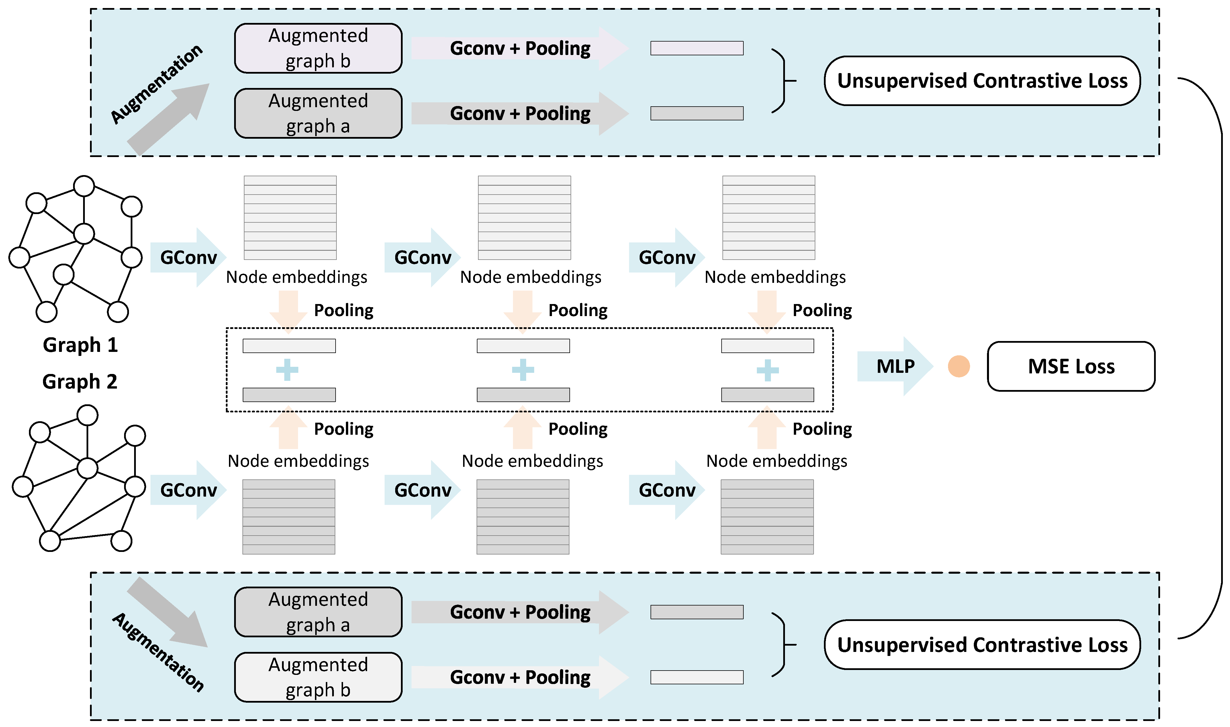
3.3. Contrastive Learning

To obtain the labels for learning graph similarity, existing works adopt traditional exact algorithms to compute the GED distance between two graphs [7]. Nevertheless, as mentioned above, these algorithms tend to require extremely longer running time given larger graphs. Consequently, the ground-truth labels are actually lacking and difficult to obtain.

To mitigate this issue, we propose an unsupervised contrastive loss to learn expressive graph representations and help predict more accurate similarity scores. Contrastive learning aims to make graph representations agree with each other under proper transformations [47]. Hence, by maximizing the agreement between two augmented views of the same graph via a contrastive loss in the latent space, more expressive and generalizable graph embeddings can be learned in the absence of labeled data. The learned embeddings can further facilitate downstream applications, such as the graph similarity computation task in this work. Next, we first introduce the graph augmentation strategy and then present the unsupervised contrastive loss.

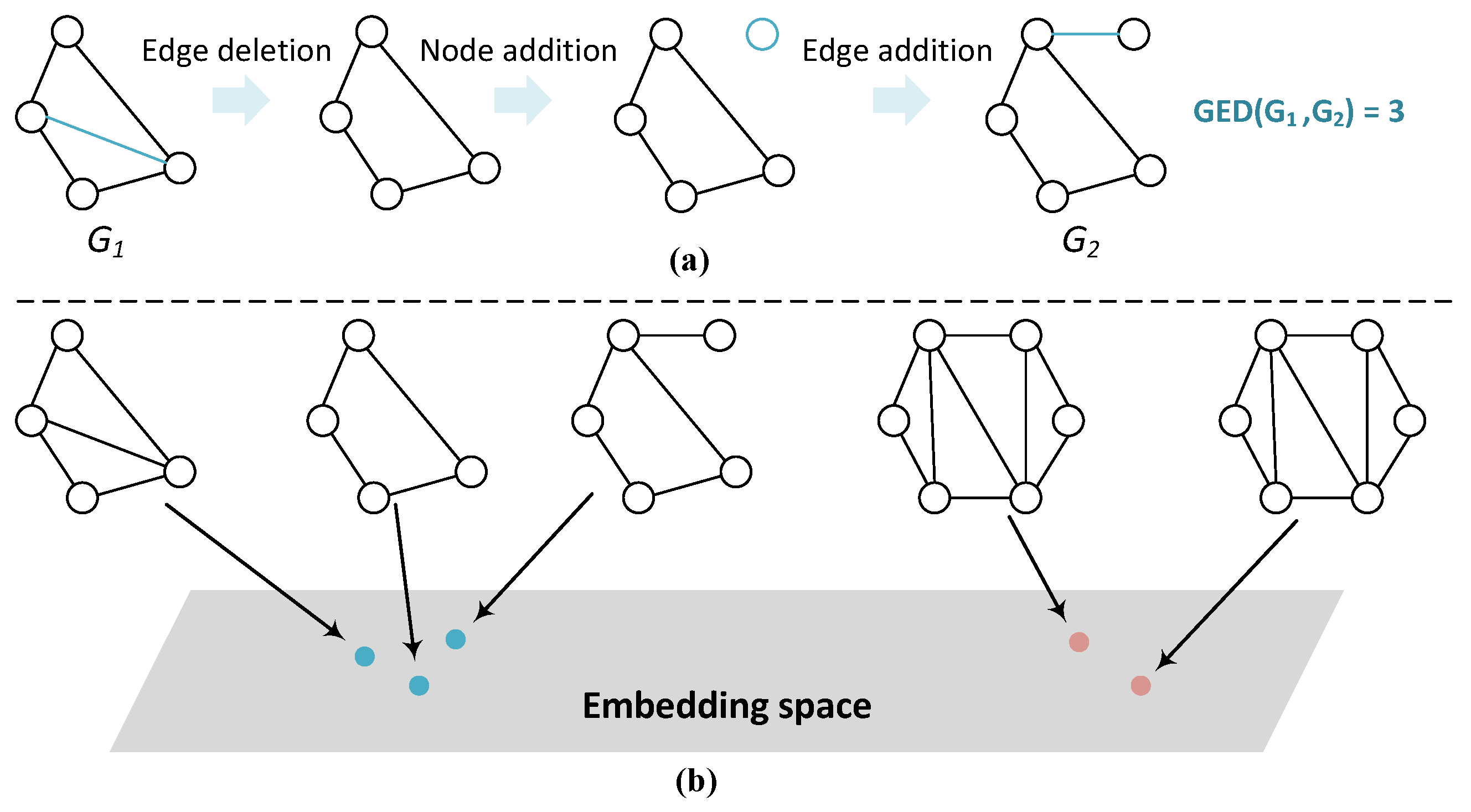
3.3.1. Graph Augmentations

Data augmentation is the prerequisite for contrastive learning, which creates new data without hurting the semantics. In the context of graphs, typical augmentation strategies include the modifications of nodes, edges, and node/edge labels [48]. In this work, inspired by previous works [47], given a graph G, we make augmentations by randomly removing nodes with probability $p_r$, randomly adding or removing edges with probability $p_e$ and masking node and edge labels with probability $p_m$, resulting in two augmented graphs, i.e., ${\widehat{G}}_a$ and ${\widehat{G}}_b$.

3.3.2. Unsupervised Contrastive Loss

After obtaining the augmented graphs for G, i.e., ${\widehat{G}}_a$ and ${\widehat{G}}_b$, we first process them with graph convolutional layers and the attention-based pooling function, generating the graph representations ${\mathit{g}}_a$ and ${\mathit{g}}_b$. Note that we adopt the same convolutional layers and pooling functions as in the graph similarity prediction network, and the graph embeddings generated by all layers are concatenated to produce ${\mathit{g}}_a$ and ${\mathit{g}}_b$.

Then, we use another multiplayer perceptron to project the graph embeddings to another latent space, i.e., ${\mathit{h}}_a=\overline{MLP}\left({\mathit{g}}_a\right)$, ${\mathit{h}}_b=\overline{MLP}\left({\mathit{g}}_b\right)$, where $\overline{MLP}$ is different from the one used in Equation (3). Finally, we devise a contrastive loss to maximize the agreement between positive pairs and increase the disagreement between negative ones. Specifically, we consider (${\widehat{G}}_a$, ${\widehat{G}}_b$) as the positive pair and ${\widehat{G}}_a$/${\widehat{G}}_b$ with other augmented graphs in the same training batch as negative pairs. The contrastive loss can be formally written as:

$$L_c=-\frac{1}{M}\sum _{i=1}^{M}log\frac{exp(cos({\mathit{h}}_{i,a},{\mathit{h}}_{i,b}))}{{\sum }_{j=1,j\ne i}^{N}exp(cos({\mathit{h}}_{i,a},{\mathit{h}}_{j,b}))},$$

(4)

where $cos(·,·)$ denotes the cosine similarity between two embeddings, $exp(·,·)$ refers to the exponential function and M represents the number of graphs in the training batch.

3.4. Training

We combine the MSE loss generated by the graph similarity prediction network and the unsupervised contrastive losses to train our proposed neural network. The overall loss function is written as:

$$L=L_s+\beta (L_c^1+L_c^2),$$

(5)

where $\beta$ is the hyperparameter that controls the contribution of the two loss functions. $L_c^1$ and $L_c^2$ represent the contrastive loss functions for the two graphs, respectively, and $L_s$ refers to the alignment loss.

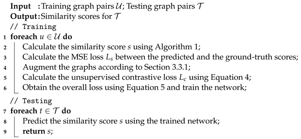
3.5. Algorithmic Descriptions

We provide the algorithm of the graph similarity prediction network in Algorithm 1 and present the general algorithm of Conga in Algorithm 2.    

Algorithm 1: Graph similarity prediction network.

Input : Two input graphs: ${\mathcal{G}}_1$ and ${\mathcal{G}}_1$

Output: Similarity score: s

1 Generate the node embeddings via graph convolutional layer, i.e., Equation (1)

2 Generate the graph embeddings via attention-based pooling, i.e., Equation (2)

3 Calculate the graph–graph similarity score s, i.e., Equation (3)

4 return s;

Algorithm 2: Algorithmic description of Conga

4. Experiments and Results

In this section, we first introduce the experimental settings. Next, we provide the empirical results and discuss the performance. Finally, we conduct further experiments.

4.1. Experimental Settings

In this subsection, we introduce the experimental settings, including the datasets, evaluation metrics, parameter settings and the baseline models.

4.1.1. Datasets

Following the state-of-the-art works [27], we adopt three real-world datasets for evaluation, including:

• AIDS [49], a dataset consisting of molecular compounds from the antiviral screen database of active compounds. The molecular compounds are converted to graphs, where atoms are represented as nodes and covalent bonds are regarded as edges. It comprises 42,687 chemical compound structures, where 700 graphs were selected and used for evaluating graph similarity search;
• LINUX [50], a dataset consisting of program dependence graphs in the Linux kernel. Each graph represents a function, where statements are represented as nodes and the dependence between two statements are represented as edges. A total of 1000 graphs were selected and used for evaluation;
• IMDB [51], a dataset consisting of ego-networks of film stars, where nodes are people and edges represent that two people appear in the same movie. It consists of 1500 networks.

More statistics of the dataset can be found in Table 2 (The datasets can be obtained from https://github.com/yunshengb/SimGNN, (accessed on 1 September 2021).) For each dataset, we create the training, validation and testing sets by following the 60%:20%:20% ratio. For AIDS and LINUX, the ground-truth GED distance is obtained by using the ${\mathtt{A}}^{*}$ algorithm [8]. Since the IMDB dataset contains larger graphs and the exact algorithms fail to work, approximate algorithms, i.e., HED [10], Hungarian [21] and VJ [22] are used to calculate the GEDs, where the minimum value is regarded as the ground-truth label [7].

Table 2. Dataset statistics. # denotes the number of objects. A. N. and A. E. represent the average number of nodes and edges, respectively. Label denotes whether the graphs are labeled.

Dataset	Contents	#Graphs	#Pairs	#A. N.	# A. E.	Label
AIDS	Molecular Compounds	700	490 K	8.9	8.8	Yes
LINUX	Program Dependence Graph	1000	1 M	7.53	6.94	No
IMDB	Film Star Ego-Networks	1500	2.25 M	13	65.94	No

4.1.2. Evaluation Metrics

We follow previous works and use mean squared error (mse), Spearman’s rank correlation coefficient ($\rho$) and precision@10 (p@10) as the evaluation metrics. Among them, mse measures the average squared difference between the ground-truth and the predicted graph similarity scores. The remaining two are used to evaluate the ranking results, where database graphs are ranked according to the similarities to the query graph. Graphs with higher similarities are assigned with lower ranks. $\rho$ characterizes the correlations between the ground-truth and predicted ranking results, and p@10 is computed by dividing the intersection of ground-truth and predicted top-10 results by 10.

4.1.3. Parameter Settings

Regarding the graph similarity prediction network, we use three convolutional layers and use ReLU as the activation function $\sigma$. The dimension of node embeddings generated by all layers is set to 100. For attention-based pooling, ${\sigma }_p$ is set to the sigmoid function, and the dimension of graph-level embedding is set to 100. $MLP$ consists of four fully connected layers with ReLU activation function, which reduces the dimensions from 600 to 200, 200 to 100, 100 to 50 and 50 to 1, which is then processed by a sigmoid function to predict the similarity score. As to the contrastive learning module, we set $p_r$, $p_e$ and $p_m$ to 0.1 and randomly choose one of the three methods when augmenting the original graph. $\overline{MLP}$ consists of two fully connected layers with ReLU activation function, where the dimension of embeddings is kept as 300. $\beta$ is set to 0.5. We set the batch size to 1024 and the learning rate to 0.001. All the hyperparameters are tuned on the validation set. The experiments are conducted on a personal computer with the Ubuntu system, an Intel Core i7-4790 CPU, an NVIDIA GeForce GTX TITAN X GPU and 32 GB memory.

It is noteworthy that, since the nodes in AIDS are labeled, we use one-hot embeddings as the initial node embeddings. For LINUX and IMDB, where nodes are unlabeled, we use a constant encoding scheme [7].

4.1.4. Baseline Models

We compare with three categories of methods. The first one includes the classical methods, including ${\mathtt{A}}^{*}$ [8], which computes exact GED distance, and Beam [15], Hungarian [21], VJ [22] and HED [10], which calculate approximate GED values.

The second one comprises state-of-the-art GNN-based methods, including:

• SimGNN [7], which uses a histogram function to model the node–node interactions and supplement with the graph-level interactions for predicting the graph similarity;
• GMN [26], which computes the similarity score through a cross-graph attention mechanism to associate nodes across graphs;
• GraphSim [13], which estimates the graph similarity by applying a convolutional neural network (CNN) on the node–node similarity matrix of the two graphs;
• GOTSim [20], which formulates graph similarity as the minimal transformation from one graph to another in the node embedding space, where an efficient differentiable model training strategy is designed;
• MGMN [14], which models global-level graph–graph interactions, local-level node–node interactions, and cross-level interactions, constituting a multilevel graph matching network for computing graph similarity. It has two variants, i.e., SGNN, a siamese graph neural network to learn global-level interactions and NGMN, a node–graph matching network for effectively learning cross-level interactions;
• ${\mathtt{H}}^{\mathtt{2}}\mathtt{MN}$ [27], which learns the graph representations from the perspective of hypergraphs, and thus captures rich substructure similarities across the graph. It has two variants, i.e., ${\mathtt{H}}^{\mathtt{2}}{\mathtt{MN}}_{\mathtt{RW}}$, which uses random walks to construct the hypergraphs and ${\mathtt{H}}^{\mathtt{2}}{\mathtt{MN}}_{\mathtt{NE}}$, which uses node neighborhood information to build the hypergraphs.

The third category combines traditional and neural models for computing the graph similarity:

• GENN-${\mathtt{A}}^{*}$ [28], which uses dynamic node embeddings to improve the branching process of the traditional A* algorithm;
• Noah [29], which combines A* search algorithm and graph neural networks to compute approximate GED, where the estimated cost function and the elastic beam size are learned through the neural networks.

4.2. Experimental Results

In this subsection, we first report the main results. Then, we conduct the ablation study. Finally, we compare the efficiency of algorithms.

4.2.1. Main Results

The main experimental results are presented in Table 3. As the classical ${\mathtt{A}}^{*}$ algorithm can calculate the exact GED on smaller datasets, i.e., AIDS and LINUX, it attains perfect results on these two datasets. However, it cannot scale to the IMDB dataset. The classical algorithms that compute the approximate GED values, i.e., Beam, Hungarian, VJ and HED, attain relatively poorer results compared with methods involving neural networks. Nevertheless, it should be noted that these classical methods can explicitly predict the edit distance, while the pure neural methods cannot. Additionally, the solutions generated by these methods are upper bounds of the optimal GED values, while neural models predict the values at both sides of the optimal ones.

Table 3. Main experimental results (mse is in the scale of the 10${}^{-3}$). ↓ means lower values are preferred, while ↑ means higher values are preferred. / represents that the results cannot be obtained due to excessive running time or are not provided in the original work (and cannot be reproduced).

Datasets	AIDS			LINUX			IMDB
Metrics	mse(↓)	$\mathbf{\rho }$(↑)	p@10(↑)	mse(↓)	$\mathbf{\rho }$(↑)	p@10(↑)	mse(↓)	$\mathbf{\rho }$(↑)	p@10(↑)
${\mathtt{A}}^{*}$	0.000	1.000	1.000	0.000	1.000	1.000	/	/	/
Beam	12.090	0.609	0.481	9.268	0.827	0.973	2.413	0.905	0.813
Hungarian	25.296	0.510	0.360	29.805	0.638	0.913	1.845	0.932	0.825
VJ	29.157	0.517	0.310	63.863	0.581	0.287	1.831	0.934	0.815
HED	28.925	0.621	0.386	19.553	0.897	0.982	19.400	0.751	0.801
SimGNN	1.376	0.824	0.400	2.479	0.912	0.635	1.264	0.878	0.759
GMN	4.610	0.672	0.200	2.571	0.906	0.888	4.422	0.725	0.604
GraphSim	1.919	0.849	0.446	0.471	0.976	0.956	0.743	0.926	0.828
GOTSim	1.180	0.860	0.870	2.125	0.920	0.860	2.960	0.850	0.730
SGNN	2.822	0.765	0.289	11.830	0.566	0.226	1.430	0.870	0.748
NGMN	1.191	0.904	0.465	1.561	0.945	0.743	1.331	0.889	0.805
MGMN	1.169	0.905	0.456	0.439	0.985	0.955	0.335	0.919	0.837
${\mathtt{H}}^{\mathtt{2}}{\mathtt{MN}}_{\mathtt{RW}}$	0.957	0.877	0.517	0.227	0.984	0.953	0.308	0.912	0.861
${\mathtt{H}}^{\mathtt{2}}{\mathtt{MN}}_{\mathtt{NE}}$	0.913	0.881	0.521	0.105	0.990	0.975	0.589	0.913	0.889
Noah	1.545	0.734	0.809	/	/	/	27.818	0.810	0.354
GENN-${\mathtt{A}}^{*}$	0.839	0.953	0.866	0.324	0.991	0.962	/	/	/
Conga	0.823	0.892	0.550	0.121	0.992	0.987	0.288	0.948	0.871
w/o CL	0.840	0.890	0.544	0.126	0.992	0.994	0.315	0.947	0.866

As for the GNN-based regression methods, i.e., SimGNN, GMN, GraphSim, GOTSim, SGNN, NGMN, MGMN and ${\mathtt{H}}^{\mathtt{2}}\mathtt{MN}$, they achieve better results than the traditional ones. Among them, ${\mathtt{H}}^{\mathtt{2}}\mathtt{MN}$ is the best performing solution, validating the usefulness of modeling substructure interactions. After combining the classical and neural models, the ranking performance of Noah and GENN-${\mathtt{A}}^{*}$ increases, while the mse drops slightly. Additionally, both Noah and GENN-${\mathtt{A}}^{*}$ cannot effectively handle the IMDB dataset.

Our proposed method, Conga, attains the best overall performance, especially on the larger dataset IMDB. On smaller datasets, it also attains leading results. Its ranking results on AIDS is lower than GENN-${\mathtt{A}}^{*}$ and GOTSim, which can be partially attributed to the fact that it focuses more on estimating the correct GED distance. Additionally, its mse results is slightly inferior to ${\mathtt{H}}^{\mathtt{2}}{\mathtt{MN}}_{\mathtt{NE}}$ on the LINUX dataset. That being said, its performance is more robust and consistent across all datasets/metrics.

4.2.2. Ablation Results

We further conduct an ablation study to validate the effectiveness of our proposed modules. Specifically, we remove the contrastive learning module and report the results of the graph similarity prediction network, i.e., Conga w/o CL in Table 3. It is evident that without the contrastive learning, the results of most metrics drop across all datasets, especially on the larger dataset IMDB. This can be ascribed to the more expressive entity representations induced by the unsupervised contrastive loss.

Furthermore, we can observe that even without the contrastive learning module, the vanilla graph similarity prediction network can also attain state-of-the art performance compared with existing methods. This shows that merely modeling the graph-level interactions can already achieve superior prediction results, despite that the intricate node-level and substructure-level information is discarded. Additinally, we reveal in the following section that our design is much more efficient than present methods that aim to capture fine-grained information. It is noteworthy that, instead of claiming that node–node and substructure–substructure are useless, we aim to demonstrate that only modeling the graph-level interaction can already achieve both high effectiveness and efficiency.

4.2.3. Efficiency Comparison

We further compare the efficiency of these approaches. It can be seen from Table 4 that our proposed framework, Conga, requires the least running time, which is over 30× faster than the classic methods and 3× faster than the neural methods. This is due to its simple architecture that merely comprises convolutional layers and pooling functions, where the resource-consuming fine-grained interactions between graphs are abandoned. In addition, it shows that the contrastive learning module brings extra running time.

Table 4. Efficiency comparison. The values denote average time consumption on one pair of graphs in milliseconds. / represents that the results cannot be obtained due to excessive running time or are not provided in the original work (and cannot be reproduced).

Methods	AIDS	LINUX	IMDB	Methods	AIDS	LINUX	IMDB
SimGNN	5.3	5	6.6	${\mathtt{A}}^{*}$	1324.7	896.3	/
GMN	7	7.1	9.1	Beam	13.2	9.5	119.4
GraphSim	7.5	7.5	8.1	Hungarian	8.2	6.8	105.6
MGMN	5.2	5.6	7.1	VJ	9	7.4	109.1
${\mathtt{H}}^{\mathtt{2}}\mathtt{MN}$	0.9	0.8	1.2	Noah	>10.0	/	>100.0
Conga	0.3	0.3	0.3	GENN-${\mathtt{A}}^{*}$	>10.0	>10.0	/
w/o CL	0.2	0.2	0.2

From the table, we can also observe that, on average, the neural methods (on the left) are faster than the traditional ones or the ones that build upon traditional frameworks (on the right).

4.3. Further Analysis

We conduct further experiments to validate the effectiveness of our proposed components.

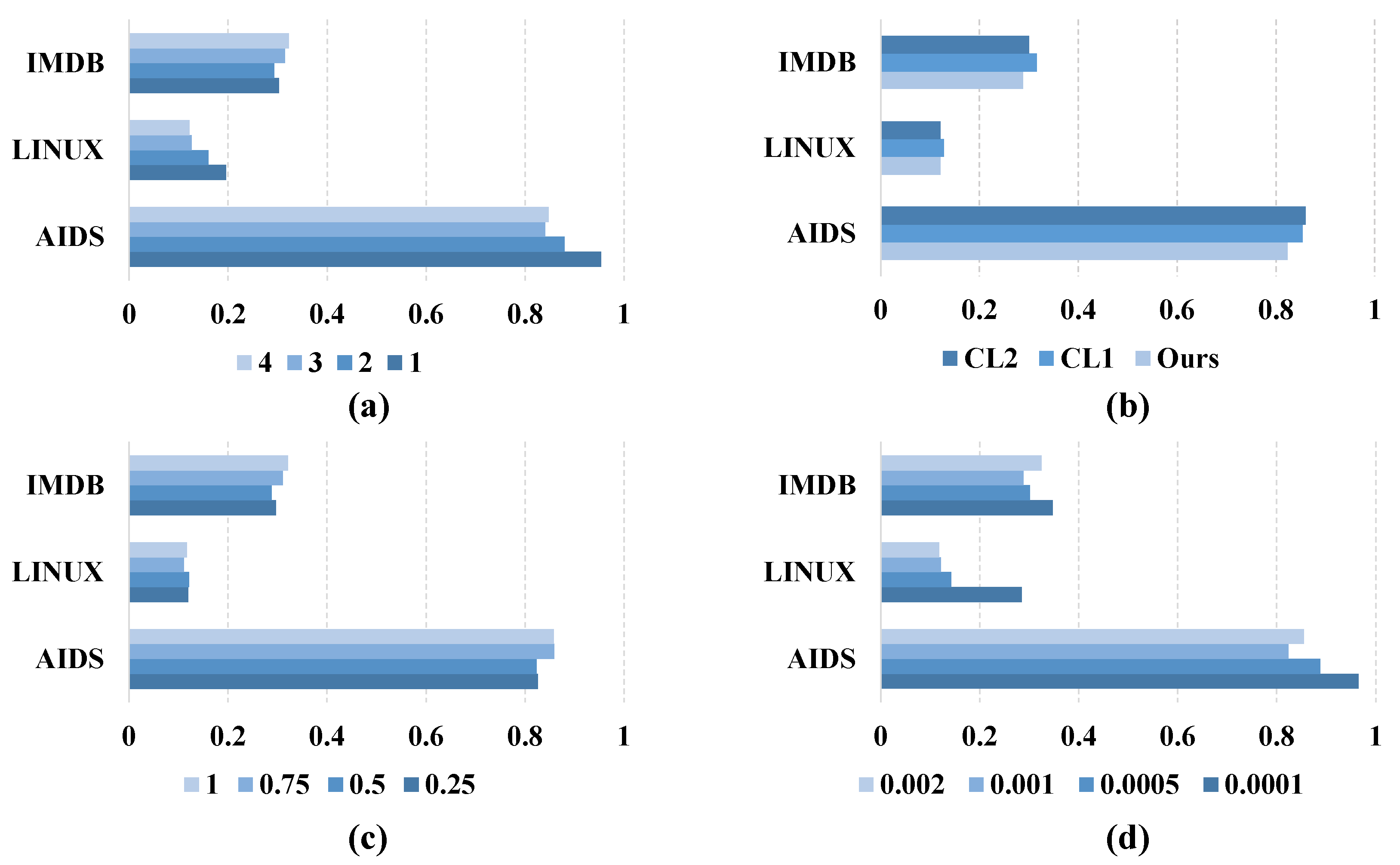
4.3.1. On GNN Layers

First, we test the influence of the number of GNN layers on the results. We change the number of GNN layers from 1 to 4 and report the mse values generated by our proposed graph similarity prediction network. As shown in Figure 3a, the number of layers does affect the overall performance. Specially, fewer layers cannot extract useful information from the graphs, leading to larger mse values on AIDS and LINUX, while too many layers would cause the overfitting issue, as pointed out by previous study, which in turn results in a higher mse on IMDB. Hence, the number of GNN layers should be set to an appropriate value.

Figure 3. Mse results of the further analysis (in the scale of the 10${}^{-3}$). Lower values are preferred. (a) Experiment on GNN layers. (b) Experiment on graph augmentation in contrastive learning. (c) Experiment on loss function. (d) Experiment on learning rate.

4.3.2. On Graph Augmentation in Contrastive Learning

Next, we examine the influence of different data augmentation strategies in contrastive learning on the results. Specifically, we aim to compare with two variants, i.e., CL1, which combines two augmentation strategies to augment the graph at each time, and CL2, which additionally introduces an augmentation strategy (that samples a subgraph from the original graph using random walk) [47].

It is observed from Figure 3b that our proposed augmentation strategy can generate the lowest mse value. This demonstrates that, for the graph similarity computation task, the augmented graph should not deviate too much from the original graph (Ours vs. CL1), and the subgraph sampling augmentation strategy does not align with the goal of GED computation (Ours vs. CL2), since a subgraph might significantly modify the original graph’s GED distance to another graph.

4.3.3. On Loss Function

Furthermore, we analyze the hyperparameter $\beta$ in Equation (5), which controls the contribution of supervised similarity prediction loss and the unsupervised contrastive loss. As shown in Figure 3c, generally speaking, a lower $\beta$ is preferred, since the contrastive learning module mainly helps to learn more expressive embeddings and does not directly influence the similarity computation. Hence, importance should still be placed on the similarity prediction. Nevertheless, setting $\beta$ to 0.25 brings higher mse compared with 0.5 on IMDB, showing that contrastive learning still plays a significant role in the overall loss function.

4.3.4. On Learning Rate

Finally, we investigate the influence of the learning rate of the training process. It is observed from Figure 3d that the learning rate is critical to the overall performance. As thus, in our experiment, we carefully tune the hyperparameter on the validation set and set the learning rate to 0.001.

5. Conclusions and Future Works

In this work, we put forward a contrastive neural graph similarity calculation framework, i.e., Conga, so as to mitigate the reliance on labeled data and meanwhile enhance the computation efficiency. Experimental results on three public datasets validate that Conga can attain the best overall performance across different evaluation metrics. In the meantime, Conga largely speeds up the graph similarity computation process. This reveals that our proposed strategy can be a competitive candidate for real-world applications that involve graph similarity computation.

For future works, we plan to explore more useful augmentation strategies for contrastive learning. Additionally, how to make the prediction results explainable is also worthy of investigation.

References

1. Kriegel, H.; Pfeifle, M.; Schönauer, S. Similarity Search in Biological and Engineering Databases. IEEE Data Eng. Bull. 2004, 27, 37–44. [Google Scholar]
2. Wang, S.; Chen, Z.; Yu, X.; Li, D.; Ni, J.; Tang, L.; Gui, J.; Li, Z.; Chen, H.; Yu, P.S. Heterogeneous Graph Matching Networks for Unknown Malware Detection. In Proceedings of the Twenty-Eighth International Joint Conference on Artificial Intelligence, IJCAI 2019, Macao, China, 10–16 August 2019; pp. 3762–3770. [Google Scholar]
3. Zeng, W.; Zhao, X.; Tang, J.; Lin, X.; Groth, P. Reinforcement Learning-based Collective Entity Alignment with Adaptive Features. ACM Trans. Inf. Syst. 2021, 39, 26:1–26:31. [Google Scholar] [CrossRef]
4. Zeng, W.; Zhao, X.; Tang, J.; Li, X.; Luo, M.; Zheng, Q. Towards Entity Alignment in the Open World: An Unsupervised Approach. In Proceedings of the Database Systems for Advanced Applications—26th International Conference, DASFAA 2021, Taipei, Taiwan, 11–14 April 2021; Springer: Berlin/Heidelberg, Germany, 2021; Volume 12681, pp. 272–289. [Google Scholar]
5. Bunke, H. On a relation between graph edit distance and maximum common subgraph. Pattern Recognit. Lett. 1997, 18, 689–694. [Google Scholar] [CrossRef]
6. Bunke, H.; Shearer, K. A graph distance metric based on the maximal common subgraph. Pattern Recognit. Lett. 1998, 19, 255–259. [Google Scholar] [CrossRef]
7. Bai, Y.; Ding, H.; Bian, S.; Chen, T.; Sun, Y.; Wang, W. SimGNN: A Neural Network Approach to Fast Graph Similarity Computation. In Proceedings of the Twelfth ACM International Conference on Web Search and Data Mining, WSDM 2019, Melbourne, Australia, 11–15 February 2019; pp. 384–392. [Google Scholar]
8. Hart, P.E.; Nilsson, N.J.; Raphael, B. A Formal Basis for the Heuristic Determination of Minimum Cost Paths. IEEE Trans. Syst. Sci. Cybern. 1968, 4, 100–107. [Google Scholar] [CrossRef]
9. Zeng, Z.; Tung, A.K.H.; Wang, J.; Feng, J.; Zhou, L. Comparing Stars: On Approximating Graph Edit Distance. Proc. VLDB Endow. 2009, 2, 25–36. [Google Scholar] [CrossRef] [Green Version]
10. Fischer, A.; Suen, C.Y.; Frinken, V.; Riesen, K.; Bunke, H. Approximation of graph edit distance based on Hausdorff matching. Pattern Recognit. 2015, 48, 331–343. [Google Scholar] [CrossRef]
11. Kipf, T.N.; Welling, M. Semi-Supervised Classification with Graph Convolutional Networks. In Proceedings of the 5th International Conference on Learning Representations, ICLR 2017, Toulon, France, 24–26 April 2017. [Google Scholar]
12. Ying, Z.; You, J.; Morris, C.; Ren, X.; Hamilton, W.L.; Leskovec, J. Hierarchical Graph Representation Learning with Differentiable Pooling. In Proceedings of the Advances in Neural Information Processing Systems 31: Annual Conference on Neural Information Processing Systems 2018, NeurIPS 2018, Montréal, QC, Canada, 3–8 December 2018; pp. 4805–4815. [Google Scholar]
13. Bai, Y.; Ding, H.; Gu, K.; Sun, Y.; Wang, W. Learning-Based Efficient Graph Similarity Computation via Multi-Scale Convolutional Set Matching. In Proceedings of the Thirty-Fourth AAAI Conference on Artificial Intelligence, AAAI 2020, The Thirty-Second Innovative Applications of Artificial Intelligence Conference, IAAI 2020, The Tenth AAAI Symposium on Educational Advances in Artificial Intelligence, EAAI 2020, New York, NY, USA, 7–12 February 2020; pp. 3219–3226. [Google Scholar]
14. Ling, X.; Wu, L.; Wang, S.; Ma, T.; Xu, F.; Liu, A.X.; Wu, C.; Ji, S. Multilevel Graph Matching Networks for Deep Graph Similarity Learning. IEEE Trans. Neural Netw. Learn. Syst. 2021, 1–15. [Google Scholar] [CrossRef]
15. Neuhaus, M.; Riesen, K.; Bunke, H. Fast Suboptimal Algorithms for the Computation of Graph Edit Distance; Lecture Notes in Computer Science; Springer: Berlin/Heidelberg, Germany, 2006; Volume 4109, pp. 163–172. [Google Scholar]
16. Zhao, X.; Xiao, C.; Lin, X.; Wang, W.; Ishikawa, Y. Efficient processing of graph similarity queries with edit distance constraints. VLDB J. 2013, 22, 727–752. [Google Scholar] [CrossRef]
17. Chen, Y.; Zhao, X.; Lin, X.; Wang, Y.; Guo, D. Efficient Mining of Frequent Patterns on Uncertain Graphs. IEEE Trans. Knowl. Data Eng. 2019, 31, 287–300. [Google Scholar] [CrossRef]
18. Zhao, X.; Xiao, C.; Lin, X.; Zhang, W.; Wang, Y. Efficient structure similarity searches: A partition-based approach. VLDB J. 2018, 27, 53–78. [Google Scholar] [CrossRef]
19. Raymond, J.W.; Gardiner, E.J.; Willett, P. RASCAL: Calculation of Graph Similarity using Maximum Common Edge Subgraphs. Comput. J. 2002, 45, 631–644. [Google Scholar] [CrossRef]
20. Doan, K.D.; Manchanda, S.; Mahapatra, S.; Reddy, C.K. Interpretable Graph Similarity Computation via Differentiable Optimal Alignment of Node Embeddings. In Proceedings of the SIGIR ’21: The 44th International ACM SIGIR Conference on Research and Development in Information Retrieval, Virtual Event, 11–15 July 2021; pp. 665–674. [Google Scholar]
21. Riesen, K.; Bunke, H. Approximate graph edit distance computation by means of bipartite graph matching. Image Vis. Comput. 2009, 27, 950–959. [Google Scholar] [CrossRef]
22. Fankhauser, S.; Riesen, K.; Bunke, H. Speeding Up Graph Edit Distance Computation through Fast Bipartite Matching; Lecture Notes in Computer Science; Springer: Berlin/Heidelberg, Germany, 2011; Volume 6658, pp. 102–111. [Google Scholar]
23. Ma, G.; Ahmed, N.K.; Willke, T.L.; Yu, P.S. Deep graph similarity learning: A survey. Data Min. Knowl. Discov. 2021, 35, 688–725. [Google Scholar] [CrossRef]
24. Xu, H.; Duan, Z.; Wang, Y.; Feng, J.; Chen, R.; Zhang, Q.; Xu, Z. Graph partitioning and graph neural network based hierarchical graph matching for graph similarity computation. Neurocomputing 2021, 439, 348–362. [Google Scholar] [CrossRef]
25. Bai, Y.; Ding, H.; Sun, Y.; Wang, W. Convolutional Set Matching for Graph Similarity. arXiv 2018, arXiv:1810.10866. [Google Scholar]
26. Li, Y.; Gu, C.; Dullien, T.; Vinyals, O.; Kohli, P. Graph Matching Networks for Learning the Similarity of Graph Structured Objects. In Proceedings of the 36th International Conference on Machine Learning, ICML 2019, Long Beach, CA, USA, 9–15 June 2019; Volume 97, pp. 3835–3845. [Google Scholar]
27. Zhang, Z.; Bu, J.; Ester, M.; Li, Z.; Yao, C.; Yu, Z.; Wang, C. H2MN: Graph Similarity Learning with Hierarchical Hypergraph Matching Networks. In Proceedings of the KDD ’21: The 27th ACM SIGKDD Conference on Knowledge Discovery and Data Mining, Virtual Event, 14–18 August 2021; pp. 2274–2284. [Google Scholar]
28. Wang, R.; Zhang, T.; Yu, T.; Yan, J.; Yang, X. Combinatorial Learning of Graph Edit Distance via Dynamic Embedding. In Proceedings of the IEEE Conference on Computer Vision and Pattern Recognition, CVPR 2021, Virtual, 19–25 June 2021; pp. 5241–5250. [Google Scholar]
29. Yang, L.; Zou, L. Noah: Neural-optimized A* Search Algorithm for Graph Edit Distance Computation. In Proceedings of the 37th IEEE International Conference on Data Engineering, ICDE 2021, Chania, Greece, 19–22 April 2021; pp. 576–587. [Google Scholar]
30. Hjelm, R.D.; Fedorov, A.; Lavoie-Marchildon, S.; Grewal, K.; Bachman, P.; Trischler, A.; Bengio, Y. Learning deep representations by mutual information estimation and maximization. In Proceedings of the 7th International Conference on Learning Representations, ICLR 2019, New Orleans, LA, USA, 6–9 May 2019. [Google Scholar]
31. Zeng, W.; Zhao, X.; Tang, J.; Fan, C. Reinforced Active Entity Alignment. In Proceedings of the CIKM ’21: The 30th ACM International Conference on Information and Knowledge Management, Virtual Event, 1–5 November 2021; pp. 2477–2486. [Google Scholar]
32. Jin, M.; Zheng, Y.; Li, Y.; Gong, C.; Zhou, C.; Pan, S. Multi-Scale Contrastive Siamese Networks for Self-Supervised Graph Representation Learning. In Proceedings of the Thirtieth International Joint Conference on Artificial Intelligence, IJCAI 2021, Virtual Event, 19–27 August 2021; pp. 1477–1483. [Google Scholar]
33. Hong, H.; Li, X.; Pan, Y.; Tsang, I.W. Domain-Adversarial Network Alignment. IEEE Trans. Knowl. Data Eng. 2022, 34, 3211–3224. [Google Scholar] [CrossRef]
34. Du, X.; Yan, J.; Zhang, R.; Zha, H. Cross-Network Skip-Gram Embedding for Joint Network Alignment and Link Prediction. IEEE Trans. Knowl. Data Eng. 2022, 34, 1080–1095. [Google Scholar] [CrossRef]
35. Zanfir, A.; Sminchisescu, C. Deep Learning of Graph Matching. In Proceedings of the 2018 IEEE Conference on Computer Vision and Pattern Recognition, CVPR 2018, Salt Lake City, UT, USA, 18–22 June 2018; pp. 2684–2693. [Google Scholar]
36. Zhang, Z.; Lee, W.S. Deep Graphical Feature Learning for the Feature Matching Problem. In Proceedings of the 2019 IEEE/CVF International Conference on Computer Vision, ICCV 2019, Seoul, Korea, 27 October– 2 November 2019; pp. 5086–5095. [Google Scholar]
37. Zhao, X.; Zeng, W.; Tang, J.; Wang, W.; Suchanek, F.M. An Experimental Study of State-of-the-Art Entity Alignment Approaches. IEEE Trans. Knowl. Data Eng. 2022, 34, 2610–2625. [Google Scholar] [CrossRef]
38. Zeng, W.; Zhao, X.; Wang, W.; Tang, J.; Tan, Z. Degree-Aware Alignment for Entities in Tail. In Proceedings of the 43rd International ACM SIGIR Conference on Research and Development in Information Retrieval, SIGIR 2020, Virtual Event, 25–30 July 2020; pp. 811–820. [Google Scholar]
39. Zeng, W.; Zhao, X.; Li, X.; Tang, J.; Wang, W. On entity alignment at scale. VLDB J. 2022. [Google Scholar] [CrossRef]
40. Malviya, S.; Kumar, P.; Namasudra, S.; Tiwary, U.S. Experience Replay-Based Deep Reinforcement Learning for Dialogue Management Optimisation. ACM Trans. Asian Low-Resour. Lang. Inf. Process. 2022. [Google Scholar] [CrossRef]
41. Manjari, K.; Verma, M.; Singal, G.; Namasudra, S. QEST: Quantized and Efficient Scene Text Detector Using Deep Learning. ACM Trans. Asian Low-Resour. Lang. Inf. Process. 2022. [Google Scholar] [CrossRef]
42. Agrawal, D.; Minocha, S.; Namasudra, S.; Kumar, S. Ensemble Algorithm using Transfer Learning for Sheep Breed Classification. In Proceedings of the 15th IEEE International Symposium on Applied Computational Intelligence and Informatics, SACI 2021, Timisoara, Romania, 19–21 May 2021; pp. 199–204. [Google Scholar] [CrossRef]
43. Devi, D.; Namasudra, S.; Kadry, S.N. A Boosting-Aided Adaptive Cluster-Based Undersampling Approach for Treatment of Class Imbalance Problem. Int. J. Data Warehous. Min. 2020, 16, 60–86. [Google Scholar] [CrossRef]
44. Chakraborty, A.; Mondal, S.P.; Alam, S.; Mahata, A. Cylindrical neutrosophic single-valued number and its application in networking problem, multi-criterion group decision-making problem and graph theory. CAAI Trans. Intell. Technol. 2020, 5, 68–77. [Google Scholar] [CrossRef]
45. Liu, R. Study on single-valued neutrosophic graph with application in shortest path problem. CAAI Trans. Intell. Technol. 2020, 5, 308–313. [Google Scholar] [CrossRef]
46. Chen, L.; Qiao, S.; Han, N.; Yuan, C.; Song, X.; Huang, P.; Xiao, Y. Friendship prediction model based on factor graphs integrating geographical location. CAAI Trans. Intell. Technol. 2020, 5, 193–199. [Google Scholar] [CrossRef]
47. You, Y.; Chen, T.; Sui, Y.; Chen, T.; Wang, Z.; Shen, Y. Graph Contrastive Learning with Augmentations. In Proceedings of the Advances in Neural Information Processing Systems 33: Annual Conference on Neural Information Processing Systems 2020, NeurIPS 2020, Virtual, 6–12 December 2020. [Google Scholar]
48. Trivedi, P.; Lubana, E.S.; Yan, Y.; Yang, Y.; Koutra, D. Augmentations in Graph Contrastive Learning: Current Methodological Flaws & Towards Better Practices. In Proceedings of the WWW ’22: The ACM Web Conference 2022, Virtual Event, 25–29 April 2022; pp. 1538–1549. [Google Scholar]
49. Liang, Y.; Zhao, P. Similarity Search in Graph Databases: A Multi-Layered Indexing Approach. In Proceedings of the 33rd IEEE International Conference on Data Engineering, ICDE 2017, San Diego, CA, USA, 19–22 April 2017; pp. 783–794. [Google Scholar]
50. Wang, X.; Ding, X.; Tung, A.K.H.; Ying, S.; Jin, H. An Efficient Graph Indexing Method. In Proceedings of the 2012 IEEE 28th International Conference on Data Engineering, Arlington, VA, USA, 1–5 April 2012; pp. 210–221. [Google Scholar]
51. Yanardag, P.; Vishwanathan, S.V.N. Deep Graph Kernels. In Proceedings of the 21th ACM SIGKDD International Conference on Knowledge Discovery and Data Mining, Sydney, Australia, 10–13 August 2015; pp. 1365–1374. [Google Scholar]
Publisher’s Note: MDPI stays neutral with regard to jurisdictional claims in published maps and institutional affiliations.
Article Metrics
Citations
Article Access Statistics
Multiple requests from the same IP address are counted as one view.