1. Introduction
The Baltic Sea is an important socio-economic zone for all the countries surrounding it, including Finland and Sweden. The waterbody supports not only critical and frequent transportation of goods, services, and passengers, but also crucial ecological systems [
1,
2]. Thus, it is of paramount importance for the region to maintain a high level of reliability and efficiency with respect to maritime operations in the area. A significant challenge is presented by the fact that, in the winter, large parts of the northern half of the Baltic Sea are typically ice-covered, with significant interannual variability with regard to the maximum ice extent [
3]. To mitigate these challenges and to maintain safe and efficient year-round navigation, a system known as the Finnish–Swedish Winter Navigation System (FSWNS) has been established [
4]. The system is collaboratively managed by authorities from Finland and Sweden and manages winter navigation-related challenges by the combined use of (a) ice class regulations, (b) traffic regulations, and (c) icebreaker assistance [
5]. Specifically, to make sure that ships have enough ice-going capability for safe and efficient operations, they must be built and operated following the Finnish–Swedish Ice Class Rules (FSICR) [
4]. These are enforced through port-specific traffic restrictions set by Finnish and Swedish maritime authorities in terms of the minimum ice class and deadweight needed to be eligible for icebreaker assistance [
4]. Icebreaker assistance is provided by icebreakers, i.e., vessels specially designed to navigate through ice and break an ice channel which other ships of lower ice-going capability can navigate. If necessary, an icebreaker may also assist vessels by towing. Within the FSWNS, icebreaker assistance is primarily provided by the fleet of Finnish and Swedish state-owned and operated icebreakers, including nine major Finnish icebreakers (Polaris, Fennica, Nordica, Otso, Kontio, Voima, Sisu, Urho. and Zeus of Finland) and five major Swedish icebreakers (Ale, Atle, Frej, Oden, and Ymer) [
6,
7].
In areas with frequent ship traffic, such as the Baltic Sea, icebreakers typically create and maintain a network of ice channels, often referred to as dirways (‘directed ways’). Dirways are routes defined by the icebreaking authority in the form of waypoints along which ships are advised to operate. Due to variations in prevailing wind and ice conditions, dirways are updated frequently, often at 2–14-day intervals [
8].
To reduce the amount of Green House Gasses (GHGs) emitted by ships, in 2011 the IMO adopted its Energy Efficiency Design Index (EEDI) regulations [
9]. These regulations aim to reduce the amount of GHGs from ships by promoting the use of highly energy-efficient solutions. Although the regulations target GHG emissions only, due to their technical content, they in effect limit the maximum installed propulsion power of conventional oil-powered ships and favor open water optimized hull forms Other upcoming maritime emissions limiting IMO and EU regulations have similar effect on merchant vessels. As a result, the average ice-going capability and attainable speed in ice conditions of ice-class ships may decrease. This in turn may result in an increased demand for icebreaker assistance, resulting in prolonged waiting times for icebreaker assistance. Prolonged icebreaker waiting times may have an adverse impact on the overall cost and energy efficiency of the FSWNS.
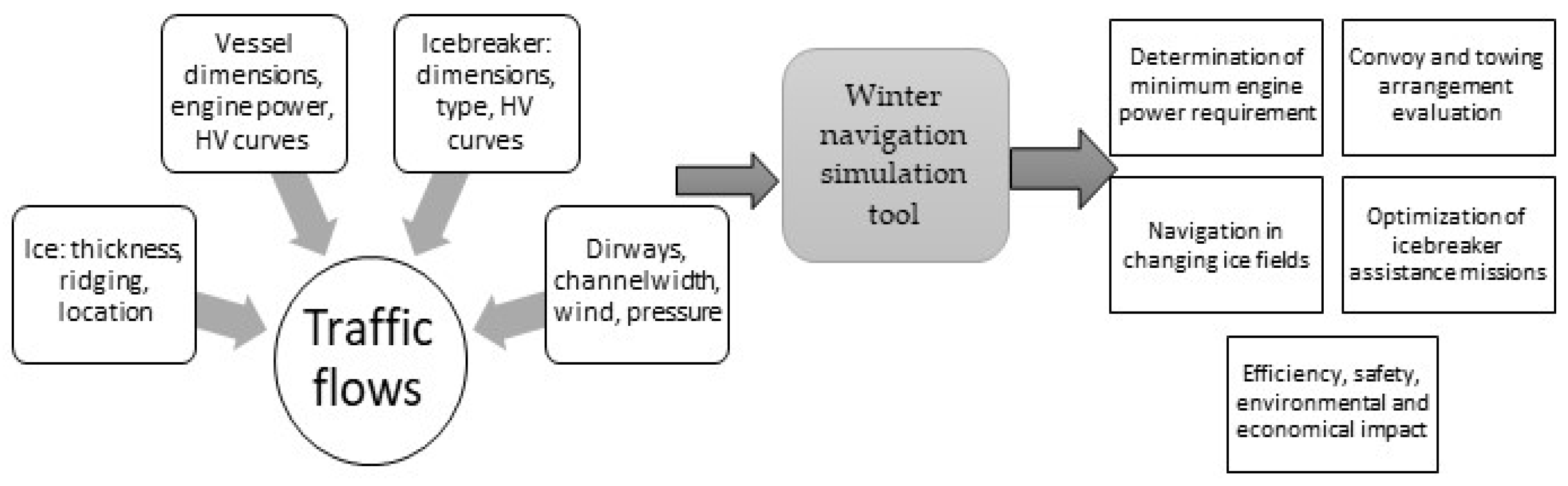
The aim of this study was to develop and validate a simulation tool that would make it possible to simulate the performance of the FSWNS under various potential future operating scenarios and thereby support decision making in matters affecting the operation and development of the FSWNS, for instance, in terms of icebreaking resources and ice class regulations. To this end, a simulation tool is outlined that mimics winter traffic flows in varying operating conditions, incorporating factors such as icebreaker scheduling and dirway changes. Icebreaker scheduling involves deciding on the number of icebreakers to be made available on any given day, their starting positions, and the assignment of operating regions for each of them. Along with simulation modelling at transport system level, mathematical modelling is used at ship level, to capture the effect of individual vessels’ interactions with the prevailing ice conditions and the resulting impact on the overall traffic flows. Through closed form expressions, vessel speed has been calculated for various ice conditions and situations, such as convoys and towing. The proposed tool will allow users to test and analyze how the FSWNS performs in any number of hypothetical (what-if) scenarios, providing an enhanced understanding of the behavior of the system. This work aims at using the strengths of simulation modelling along with the domain knowledge expertise of mariners.
Figure 1 shows a schematic block diagram of the simulation tool.
The simulation tool is implemented using a combination of discrete-event and agent-based simulation, along with process flow modelling. This choice of modelling techniques allows for the visualization of the simulation processes and results, the incorporation of stochastic elements, and a relatively fast execution time (~5 min per simulated operating month). The behavior of individual entities of the FSWNS, such as individual merchant vessels, icebreakers, and ports, are modelled using an agent-based framework, including details of their decision-making logic. Each entity (vessel or icebreaker) has several decisions to make during the winter, reacting to the changing parameters. The decision-making logic for each entity involves a set of rules in the if-then-else format, where entities change their speed, direction, and mode of operation based on system parameter values. Additionally, for the icebreakers, there is an optimization logic for deciding on the best course of action in assisting vessels.
This article is organized as follows. In
Section 2, prior work in this field is reviewed and comparisons are made between the different aspects of each piece of research. In
Section 3, first, the parameters of the system are introduced and categorized. Next, the tool schematic is presented, and the different components of the decision-support tool are highlighted. Finally, the simulation principle is described.
2. Related Work
Previously presented computer-based models for the simulation of winter navigation operations are listed in
Table 1. As per the table, the models are compared with regard to their features and capabilities, including the following: (a) whether the model can visualize the simulated operations, (b) whether the model determines the speed of ships as a function of the prevailing ice conditions, (c) whether the model provides the means to optimize the simulated system (e.g., with regard to icebreaker waiting times), (d) whether the model can consider dynamically changing ice conditions.
Tarovik 17 June 2022 (2017) [
13] present a multi-disciplinary approach for the modelling of winter navigation traffic, with a focus on the Arctic region. Both the authors’ work and the work by Tarovik et al. model ports that use geo-information system (GIS) environments for agents and object-oriented (OO) programming for coding independent sub-models that are executed dynamically during a simulation run. The authors of this article as well as Tarovik et al. present a dynamic simulation model to capture vessel and icebreaker movements along with ice conditions. Their primary aim, however, is to demonstrate an integrated software platform and its potential in addressing maritime transport system problems. They describe in detail the different disciplines and software systems that are used and how they are integrated in their application in two case studies. In comparison, the authors’ work is focused on modelling the winter navigation system in detail to develop a decision-support tool. To this end, we consider several additional parameters related to ice and vessel–icebreaker interactions. Tarovik et al. presents a generalized tool that has the potential to address a wide range of maritime topics on a holistic level. The authors’ work, on the other hand, is a highly specialized tool, considering a multitude of local factors, that addresses specific issues in winter navigation. Both models have optimization capabilities. In Tarovik et al.’s model, vessel fleet optimization, ice route optimization, and ship-design optimization capabilities are present. The authors’ work’s main emphasis is on icebreaker behavior. The focus is on optimizing tactical, strategic, and operational decisions that icebreakers need to make throughout the winter based on changing operating and traffic conditions.
Lindeberg et al. (2018) presented a deterministic simulation tool for analysis of the performance of the FSWNS in terms of ships’ cumulated waiting time for icebreaker assistance under specific operating conditions. A validation of the tool based on real-life data indicated that it is reasonably accurate. An apparent weakness of the tool is that it is impractical for the analysis of a wide range of different operating scenarios, both because modification of the assumed ice conditions and dirway configuration appears laborious and because the run time of a typical simulation is long (e.g., a simulation of one month of operations takes around 24 h). Other limitations of the tool include limited insight into the simulation process and no optimization capabilities.
Bergström and Kujala (2020) presented a discrete-event simulation-based approach for assessing the operating performance of the Finnish–Swedish Winter Navigation System (FSWNS) under different operating scenarios. Different operating scenarios were specified in terms of ice conditions, volume of maritime traffic, number of icebreakers, and regulations, such as the Energy Efficiency Design Index (EEDI). Several performance indicators were considered, including transport capacity, number of instances of icebreaker assistance, and icebreaker waiting times. A validation against real-world data on maritime traffic in the Bothnian Bay indicated that the approach could capture the complex behavior of the FSWNS and roughly estimate its operating performance. Case studies were carried out in which the approach was applied to assess the impact of replacing various percentages of the present fleet of merchant ships entering the Bay of Bothnia by EEDI-compliant ships. As per Bergström and Kujala (2020), the approach is based on a number of generalized assumptions concerning convoy operations (a maximum of two ships are assisted by an icebreaker at a time), the time it takes for an icebreaker to reach a ship in need of assistance (probabilistically determined), criteria for when icebreaker assistance is to be provided (generalized criteria), and assumptions concerning the presence of brash ice channels (generalized assumptions), among others. Other limitations of the model include: (a) no ability to visualize the simulation results, (b) no optimizing capabilities, and (c) rigid dirways.
The above-mentioned studies have demonstrated that it is feasible to simulate the operations of the FSWNS, considering key factors, such as the prevailing ice conditions, the prevailing network of dirways, the volume of ship traffic, the ice-going capabilities of individual merchant vessels, and the availability of icebreaking resources. This work aims to build on the previous work and take the concept further towards building a decision-support tool. In the field of winter navigation, most of the previous work with simulation models has involved numerical simulations that provided statistical estimates for speeds of vessels of different dimensions in varying ice conditions. The present authors’ work models traffic flows, icebreaker–vessel interactions (including convoys and towing), along with visualization. Further, the framework allows for algorithms to be embedded in the model at multiple places to intelligently capture system decision making, such as in icebreaker choice making, where an icebreaker chooses which vessel to assist next.
3. Scope of the Model
As mentioned earlier, the tool aims to help answer some of the questions regarding icebreaker operations for potential future scenarios. An important question for the stakeholders would be the determination of the number of icebreakers required with expected climatic and environmental changes. Along with the changes in ice conditions and therefore the operating speeds of vessels, the climate threat has also resulted in policy changes, which will affect the ice-going capacities of vessels. This simulation model would provide a critical bird’s-eye view of the winter navigation system.
To effectively capture the challenges of navigation, it is important to model ice conditions appropriately. There are multiple aspects of ice information, such as thickness, concentration, and topography. The information is available through ice charts published by the Finnish Meteorological Institute (FMI). However, the data are from multiple sources, such that different file formats need to be processed together to obtain a complete picture of ice conditions. The ice data are also highly dynamic and new ice information is available for each hour of each day, for every square mile of geographical area. For use in this model, this information is suitably aggregated, to ensure an acceptable compromise between the level of detail and model computational time. The vessels modeled in the simulation need to be sensitive to these ice changes and adapt their speeds (or stop) in response to the conditions. This requires a mechanism for the vessels to monitor ice parameters and evaluate their response several times during a single trip. For this, hv curves and equivalent ice thickness concepts are used. Equivalent ice thickness uses a mathematical formula that gives a single value of ice thickness based on ice concentration, thickness, and topography. The model uses the formula given by Lindeberg et al. [
14] for calculating the equivalent ice thickness. An hv curve is a polynomial regression that describes the variation in speed of a vessel as a function of ice thickness. Each vessel has an hv curve profile, based on its dimensions. The hv curves are modeled as entity attributes, and they evaluate changing speeds based on equivalent ice thickness values. Examples of hv curves are shown in
Section 4,
Figure 2.
The framework being developed is applicable to the entire Baltic Sea Region. However, to demonstrate a proof of concept and to validate the functionalities, a smaller region of high ice variation and traffic flow is selected and presented in this paper. The area of interest for this model is the Bay of Bothnia, with the Finnish and Swedish borders on either side. The traffic in this region is cooperatively managed by both Finland and Sweden. All vessel journeys calling on Finnish ports have been included. Some of these journeys originate or terminate outside the operating zone under consideration. The data have been processed to prune the vessel journeys outside the Bay of Bothnia. Following the approach of Bergström and Kujala [
15], the southern point of Kvarken was selected as an entry and exit point to and from the operational area. The case study discussed in this article focuses on operations at Finnish ports. Hence, only trips to and from Finnish ports are considered.
More details about the input data are presented in the next section.
4. Model Data
The case study presented in this article includes winter traffic from 15 January 2010 to 15 February 2010. A total of 115 vessels are incorporated. These vessels are categorized into 18 vessel types with similar hv curves. The hv curves are characterized by cubic polynomials, where the coefficients are calculated from regression formulae that have been internally established by a design company and validated against extensive measurement data [
16]. A matching algorithm has been designed to assign each vessel the most relevant hv curve profile, based (among other factors) on its dimensions and power. A detailed description of the hv curve derivation and matching is beyond the scope of this article. Knowing the ice thickness, the corresponding vessel speed can be calculated using the hv curves. A vessel’s actual speed in ice is not necessarily the same as its achievable speed (as estimated from hv curves). However, as a simplification, it has been assumed to be the same in this model. The hv curves can be used to calculate speeds under six different conditions: channel ice, level ice, floe ice, ridges, pressure, and assistance at a distance. The model is designed to include all six types. For demonstration purposes, the test cases presented in this paper have been built for an open water, level ice, and assisted at a distance condition. The level ice thickness in the model varies by area and by day. If the speed drops below the specified threshold, the vessel waits for icebreaker assistance. Once the icebreaker arrives, the speed is calculated for the “assisted at a distance” condition. This applies for all vessels and icebreakers as well, which have their own hv curves.
The traffic data used in the model have been obtained through the research project WINMOS II [
17]. The data include information about origin and destination ports; arrival, departure, and time spent at port; vessel name and type (for hv curve); and next destination. These data have been preprocessed to obtain
Table 2. The vessel itineraries used in the model are a result of AIS data processing work described in this conference article [
18]. Based on this work, it possible to know whether a ship is at port or sea. The information in
Table 2 is used an input to the simulation model. Every vessel is assigned a unique code or identifier to track its movements and KPI throughout the simulation. Similarly, every port is also assigned an identifier. The simulation also displays vessel names (anonymized) during the visualization. The departure time from the port is converted to minutes from the start of the simulation run. Since the period considered begins on 15 January 2010, midnight (0000) of 15 January is the start of the simulation run. All other departure times are relative to this starting point.
Another important component of these data is the hv curve identifier. Each vessel is assigned a vessel type, which determines the hv curves that apply to it. The hv curve code or identifier is an input to the model. Based on the code, the relevant hv curve information is referenced by the vessel during the run. The hv curve expressions for speeds in level ice (
) and the assisted at a distance condition (
) are as shown below.
In these equations,
h stands for equivalent ice thickness. The terms
a, b, and
c are the coefficients for the ice condition (curve parameters) and
w is the open water speed. A typical set of coefficients for an hv curve is shown in
Table 3.
This table corresponds to the coefficients for the vessel type “Example_ship” which has been assigned the identifier “0”. The suffix “l” is for level ice, while “d” is for the assisted at a distance condition.
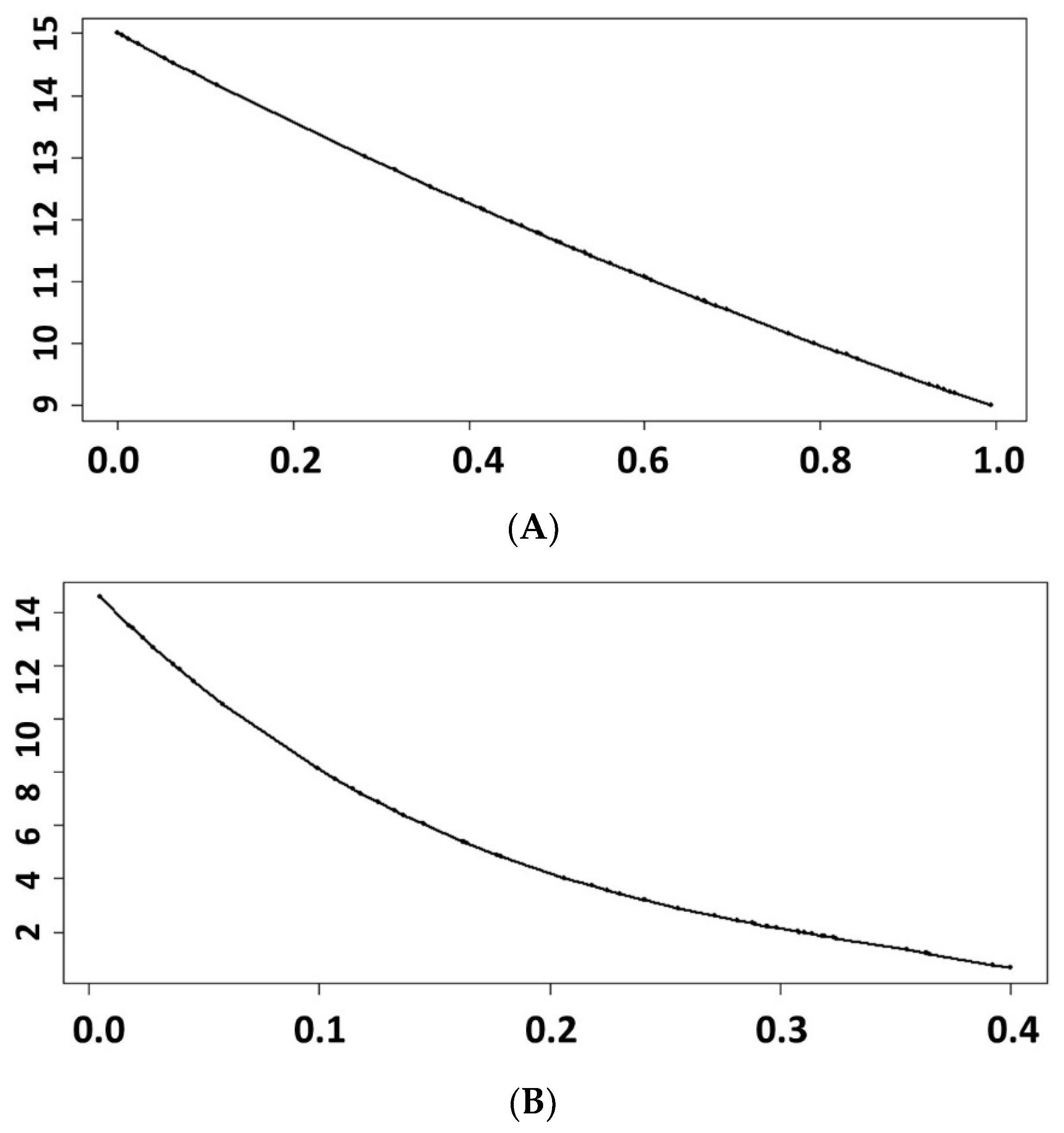
Figure 2 shows the plots of these polynomial expressions of HV curves. On the x-axis is the ice thickness, varying from 0 m (open water) to 1 m (
Figure 2A) and 0.4 m (
Figure 2B). On the y-axis is the speed achieved by the vessel in knots. As observed in both plots, the open water speed is 15 kn.
Figure 2B shows that the speed rapidly decreases with an increase in ice thickness. The speed reaches near 0 kn around 0.4 m.
Figure 2A shows that speeds of up to 9 kn can be achieved for ice thicknesses between 0.4–1 m, when the vessel is assisted by an icebreaker at a distance.
The ice data from FMI are used in two formats: SIGRID-3 and NetCDF. There are multiple fields of information for which the World Meteorological Organization (WMO) has defined standard nomenclatures and abbreviations [
19]. Ice fields can change every day, affecting the routing. The hv curves are determined with respect to level ice thickness. In the case studies, real ice data have been used to calculate equivalent ice thickness as an average of the ice concentration in a square grid. The ice data are updated every week. This updating frequency can be increased as required. Equivalent ice thickness can be defined differently depending on what ice data are available. In this article, the equivalent ice thickness is calculated using the NetCDF data, as a product of concentration and thickness, therefore maintaining volume equivalence [
20]. The equations are similar to those used in [
14,
15]. For more information, readers are pointed to [
21].
5. Modelling Framework
In this section, the underlying framework for building the decision-support tool is explained.
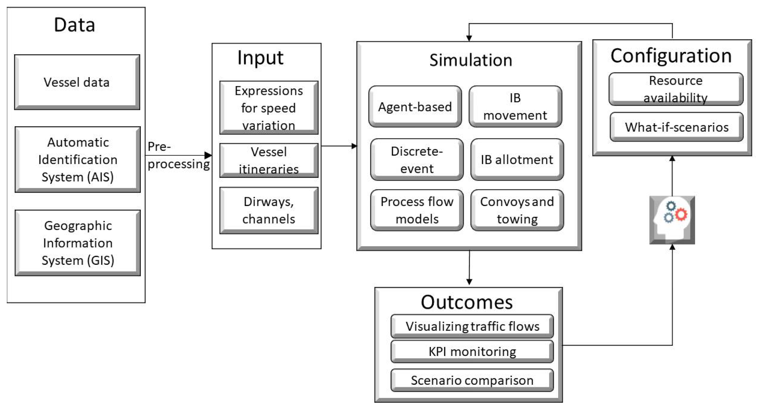
Figure 3 shows a block diagram of the proposed decision-making tool. The tool is intended to be used by experts in the domain, indicating that it is designed to complement the expertise of the user rather than to be used as a standalone tool. The expert provides key details on the availability of resources (number of icebreakers, ports operational on any given day) and other potential scenarios not captured through available data. The inputs to the model include vessel information, such as dimensions and hv-curve coefficients, traffic, and ice data. These data are processed to obtain expressions for speed variation for vessels and icebreakers, trip details (origin, destination, time of departure), ice conditions for each day, and location of dirways. The traffic data mentioned in the earlier sections are obtained by processing (Automatic Identification System) AIS data [
18]. This information is a necessary input to the simulation model. A simulation engine is at the core. It consists of agent-based models to capture the entity behaviors, discrete-event models to simulate periodic as well as randomly occurring events, and process flow models to represent vessel and icebreaker movements both at sea and in ports. Visualization is implemented, including a color-scheme to indicate varying ice thicknesses. The primary output of the simulation is a visualization of traffic flows that shows how the vessels move across changing dirways to destinations. The speeds of the vessels vary as per the ice conditions of the paths along which they are moving. The icebreakers can also be seen to assist vessels that cannot maintain a speed above the minimum specified threshold. Key Performance Index (KPI) of average waiting time is reported at the end of the simulation. The outcomes are presented to the domain expert (decision maker), who uses them for future configurations and provides feedback to the simulation.
6. Implementation
The simulation component of the tool is a standalone model developed using Anylogic® software. The model is an agent-based, discrete-event simulator with specific add-on functionalities coded using Java. The simulation provides a unified platform to integrate agents, their environments, process flows, and system uncertainties (stochastic elements). The purpose of the simulator is to mimic the operations of the FSWNS, considering all relevant underlying performance factors and attributes of the system. This tool helps compare alternative navigational scenarios to finally arrive at the most efficient combination of policies and actions. This requires modelling of traffic flows, where merchant vessels follow a predefined order of visiting multiple ports in the region. Apart from the merchant vessels, icebreakers are an important part of the winter traffic, ensuring safe operational routes for all vessels.
The environment includes varying ice conditions over the winter period. Based on ice data from FMI, ice thickness and topography can change for every mile of the sea area and as often as every day during the winter months. The paths that the vessels follow, known as dirways, are also a part of the environment. Dirways are created by icebreakers where there is ice and are subject to change due to wind, pressure, and changing ice conditions. Another aspect that needs to be captured is the transition between dirways. The ongoing journeys are completed on the old dirways and the new journeys are scheduled on the new dirways. Icebreakers need to coordinate between both set of dirways until all traffic is smoothly flowing on new dirways. This affects convoy formation as well. All these changes can affect the waiting time of the system. The speed of vessels, however, depends primarily on the ice conditions they encounter. These dynamically changing input data are modelled as events in the simulation. When an event occurs (a change in ice data or dirways), all agents are notified, and their operations are suitably modified.
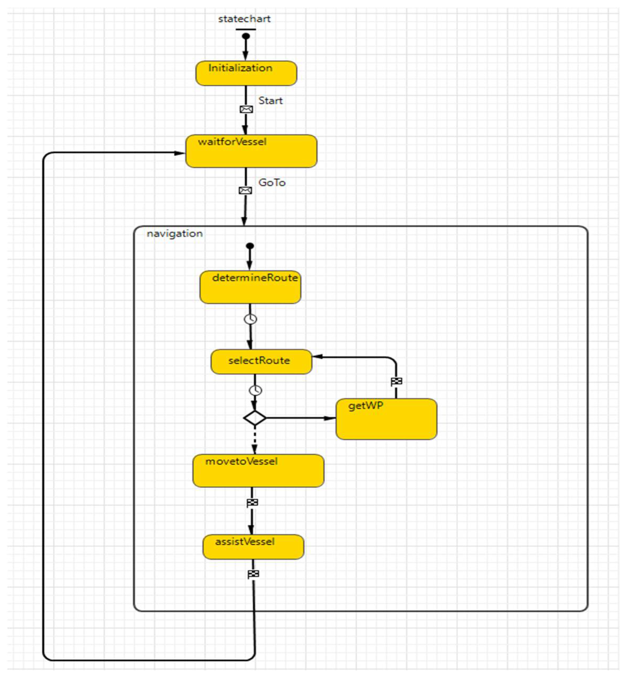
There are two agents in the model: merchant vessels and icebreakers. Statecharts are created for each agent, in which possible decisions and subsequent actions are modelled. An example is presented in
Figure 4.
At the start of the simulation, vessels enter the system representing the simulated section of the FSWNS (e.g., the Bay of Bothnia) following their schedules, at a time and place determined by real-world AIS data and the existing dirway network. The ice conditions are updated each time a ship enters a new grid square as determined by the ice data. The speeds of the vessels vary in accordance with their hv curves. When the speed of a vessel drops below a certain threshold, icebreakers are notified. Based on the location of the vessel, the icebreaker that will assist is chosen from the available fleet of icebreakers. Multiple vessels may be assisted by the same icebreakers if they are headed in the same direction. The simulation ends when all vessels in the specified time duration have run their course and completed their schedules. The vessels’ average waiting time for icebreaker assistance is one of the KPIs generated as a simulation output.
At the ports, process flow diagrams are used to model service and queuing operations. Both merchant vessels and icebreakers visit ports from time to time. From the simulation model’s perspective, depending upon the vessel type and nature of visit (whether it is a destination or a transit point), different service times are modelled. Each port has different queuing and serving capacities. Relevant probability distributions are used to model these features.
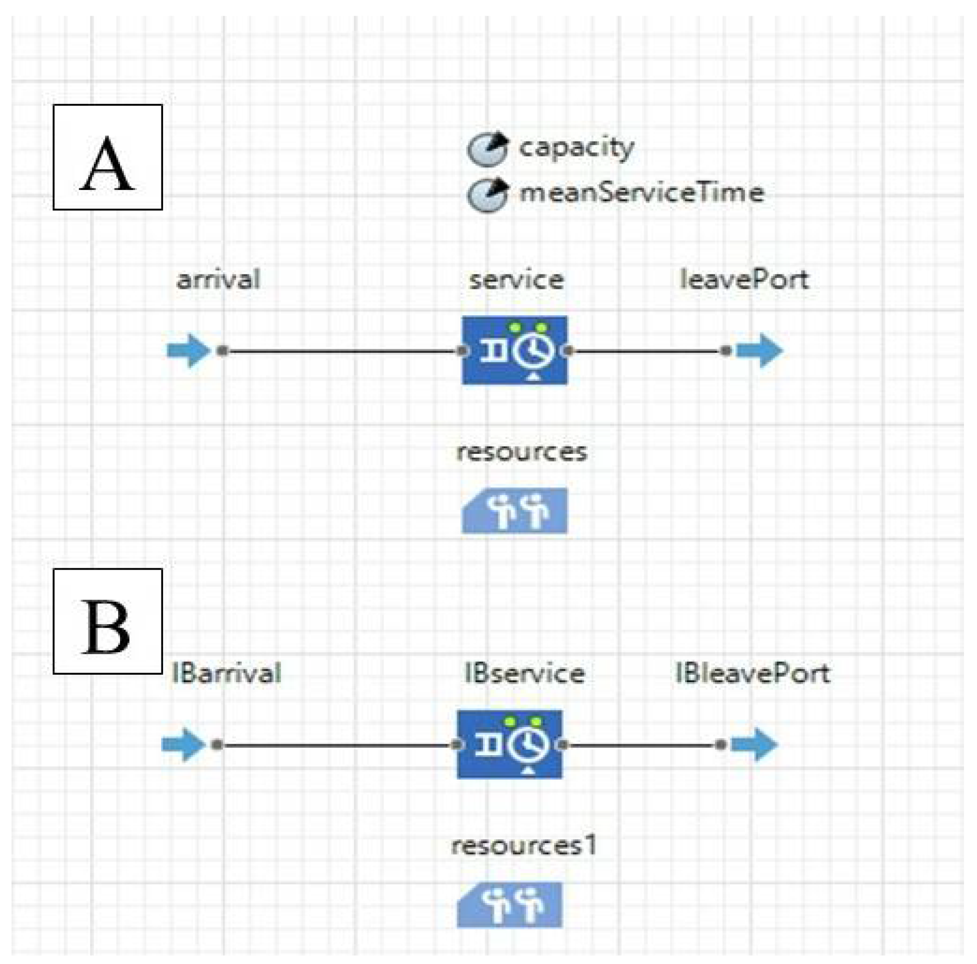
Figure 5 shows three process flows defined in the model. The first one (A) is for all merchant vessels. The service time at the port varies by vessel type and port. Each port has different resource and capacity constraints. The level of detail of service times and port constraints depends on the decisions that the end-user is interested in. In the current version, the service times of vessels have been estimated based on distributions obtained from historical data analysis. The service time (gross berthing time) is not relevant to decisions regarding icebreaker assistance as described in this article. The simulation framework here briefly shows the capability of also incorporating berthing operations-related parameters, which is a possible extension of this decision-making tool. The decisions addressed by those processes would be different from the ones mentioned in this article. However, having both these systems in one simulation model enables the user to observe interactions (if any) and capture feedback information between one process and another. Port capacities have been estimated by the practitioners and traffic controllers. In the second process flow (B), sequence of action for icebreakers at ports is modelled. Icebreakers need to regularly visit ports for crew change, provisions, and refueling. They can choose to visit any port from a list of acceptable ports. For routine visits, their downtimes are estimated from previous data, varying from 6 to 12 h. The icebreakers need to visit a port once every 10 days during the winter months. Not all icebreakers can visit a port at the same time so as to ensure that there are enough icebreakers available to support the traffic.
7. Model Functionalities
This section describes some of the key functionalities that have been implemented. More functionalities are described in a follow-up journal article. The entire operational area is divided into operating zones. These zones are defined based on ice conditions and can change dynamically over the course of a simulation run. At least one icebreaker is available in each zone. Icebreakers have specific ice-going capabilities that are modelled using hv curves. The assignment of an icebreaker to an operating zone depends on the maximum ice thickness in the region and the capabilities of the icebreaker. It is usually standard practice that wider and stronger icebreakers are assigned to the northern regions more frequently, these regions freezing sooner and for longer durations. Ice thickness is also greater in these parts, and ridging is common. The months of January–March are often considered peak winter months when the sea is frozen to the maximum extent. There are different kinds of ice: some that has formed earlier in the season, while some is freshly formed ice. All these factors affect the creation of safe navigational paths by the icebreakers. During peak winter, it is common to assign two icebreakers to the northern zones, where ice conditions are the most challenging. Apart from ice conditions, the other factor affecting the choice of the number of icebreakers is the expected traffic density in the area. Some ports are busier than the others, even during peak winters. Excessive queue build-up needs to be avoided in the areas surrounding these ports and along fairways leading to these ports. Although there are 9 Finnish icebreakers available, the actual number of active icebreakers (in service) depends on the prevailing ice conditions. For the case study described in this article, it is assumed that four icebreakers are available for the Finnish ports at any given time.
Although icebreakers are assigned to zones, they regularly coordinate with each other to ensure that the entire system operates safely and efficiently. Vessels often need assistance across multiple icebreaker zones. Typically, each icebreaker guides a vessel through its operating zone, leaving it at a safe stopping point called a waypoint. At the waypoint, the next icebreaker takes over the assistance mission and guides the vessel further along its navigational journey. Icebreakers can, however, operate outside their operating zones to ease traffic build-up or to help larger vessels that need two icebreakers. The icebreakers need to make decisions dynamically regarding which vessel to assist first, when to coordinate with another icebreaker, which path to use, and whether to build convoys (to be described later).
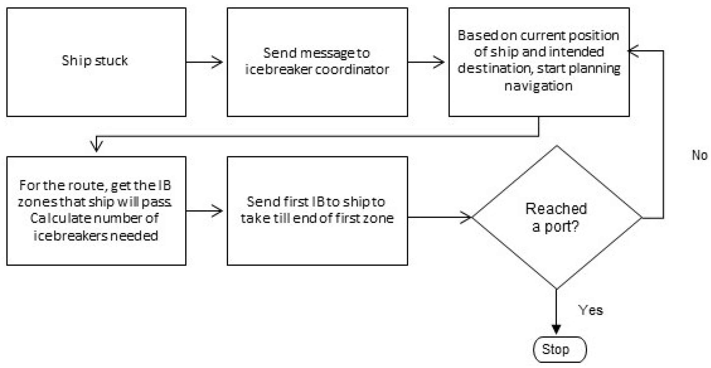
Figure 6 shows the routing logic for ships and icebreakers. When a ship is stuck, it sends out a message to the icebreaker control unit, which may be an icebreaker with a coordinating captain or a decision-making unit on land. The icebreaker in charge calculates the potential route of the vessel by considering its current position and destination. One or more icebreaker zones are identified, through which the vessel will navigate to reach its destination. A schedule is made for the vessel, which is updated each time the vessel reaches the end of a zone. The first icebreaker, that is, the icebreaker serving the first zone in which the ship is stuck, is sent to the vessel. The icebreaker leads the ship to the end of its zone or port (if the port lies in its zone). The route of the ship is reevaluated (if needed) at the end of the zone, and the next icebreaker is assigned to take the ship onward. A list of requests for each icebreaker is maintained and updated as the vessel moves from one zone to another. The vessel is removed from all lists once it reaches a port or a fairway to a port. Once the ship reaches a port, the calls to icebreakers are terminated.
Convoys
Icebreakers often try to combine trips for multiple vessels requiring assistance so that the waiting time is reduced overall. When a single icebreaker assists more than one vessel, the arrangement is known as a convoy. A convoy is different from a towing arrangement, where a vessel is physically connected to the icebreaker using mechanical links. In convoys, the icebreaker leads the way for a group of vessels to follow. There are multiple factors in deciding how many vessels can be part of a convoy. The convoy travels at the speed of the slowest vessel; hence, the icebreaker needs to ensure that the minimum speed of the convoy is greater than the threshold. If the speed of a convoy is less than “x” knots (default is 6), then the slowest vehicle is left behind. In practice, the slowest vessel may be taken up for towing by the icebreaker and the rest of the vessels may follow in a convoy. However, this case is not considered in the current model. The current model considers conventional convoys, with one icebreaker clearing a path for one or more merchant vessels. There are other convoys possible where a group of vessels follows a towed vessel or a wide vessel convoy with two icebreakers involved. These are not considered in the present model. While forming a convoy, the travel paths of the vessels are also considered. An icebreaker leading a convoy does not escort each individual vessel to its destination ports. Safe waypoints are identified where convoys can be dismantled and reformed if required with different vessels. It is possible that due to convoy formations one or more vessels end up taking a longer route to their destinations. However, keeping in mind the overall waiting time in the system, the longer route with convoys ends up being more efficient.
8. Verification and Validation of the Simulation Model
To gauge the efficacy of the model and to build trust in its functionalities, verification and validation are required. In the verification process, it is determined whether model implementation and associated data accurately represent the conceptual description and specifications. In the validation process, it is determined how accurately the simulation model and its associated data represent the real world from the perspective of the end-users [
22]. In other words, verification answers the question: “Is the model right?”, while validation answers the question: “Is this the right model?”. The verification and validation of the model is carried out using accepted techniques from the simulation literature [
23]. The methods are both subjective and objective. There are three approaches commonly used in deciding the validity of the simulation model, as described by [
23]. In the first approach, the development team conducts evaluations during the model development process. The second author has helped in this evaluation. In the second approach, the users (field experts) of the model determine whether the model is satisfactory. The fourth author in this paper has helped in this process. In the third approach, a third party, independently of the development (of the simulation model) and user teams but with thorough understanding of the intended purposes of the model, evaluates the validity. The third author has helped in this evaluation. The following subsections describe the verification and validation in detail.
8.1. Verification: Adherence to Conceptual Description
The field experts participated in demonstrations where the model was run at a perceptible speed. The movements of the vessels and icebreakers were carefully inspected, along with the formation of dirways, changing ice conditions, and the formation of convoys.
Further, the vessel speeds were monitored over a small geographical area with high ice variability to ensure that the speeds were reevaluated with changing ice conditions. The dirway changes were also inspected, a change being expected every week of the runtime. When a dirway changes, there may be some vessels in transition, that have not yet reached their destinations. These vessels continue their journeys along the old dirways. All new journeys are scheduled on the new dirways. Until all previously scheduled assistance missions are complete, icebreakers navigate along both old and new dirways.
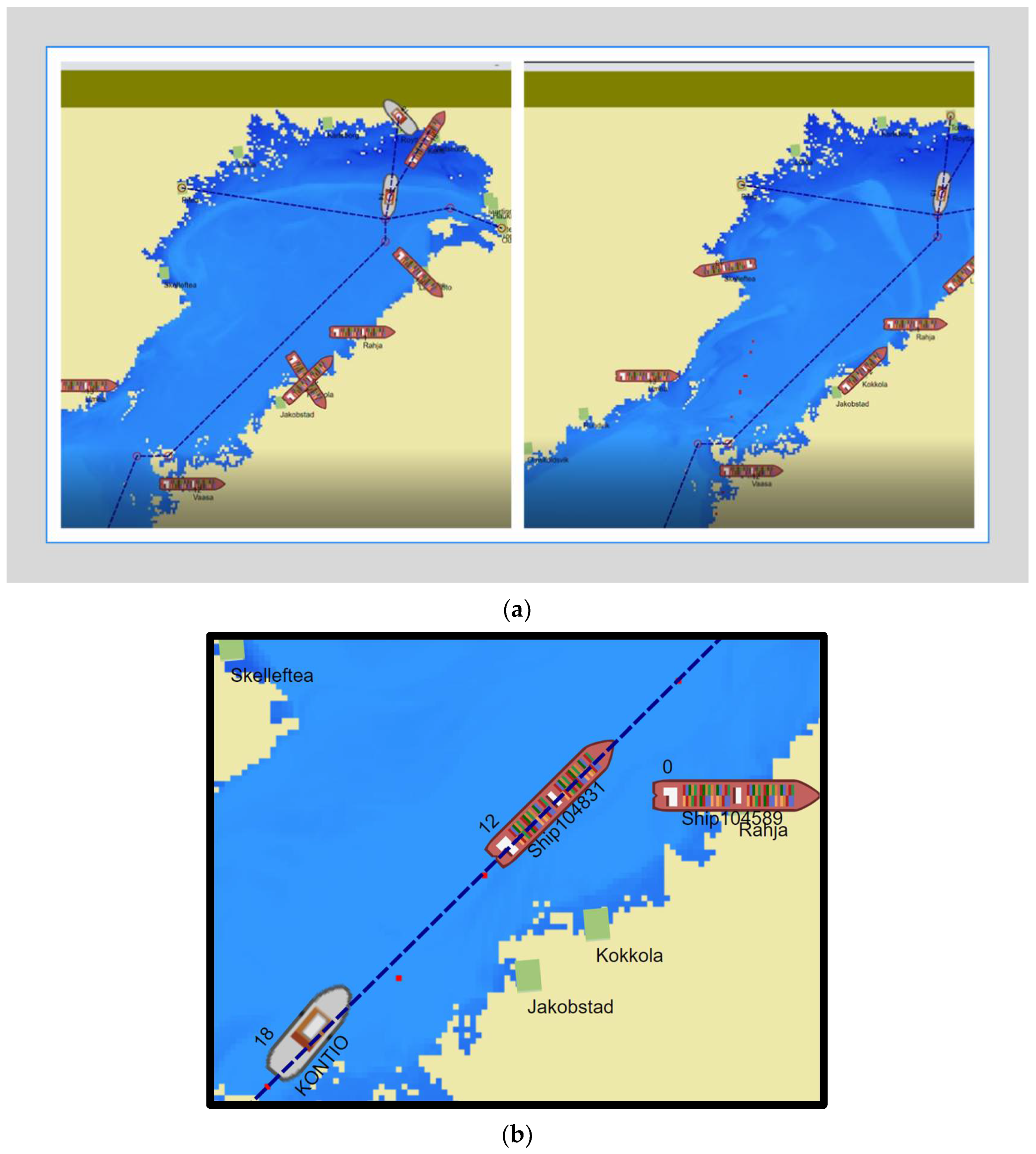
Figure 7a shows two snapshots of the visualization. To indicate varying ice thickness, different shades of blue are used in the visualization. A darker shade of blue indicates thicker ice. In
Figure 7b, the vessels and icebreakers can be visualized more clearly. For ease of inspection, the names of all vessels and icebreakers are displayed. A dynamic field for vessel speed is also displayed, indicating the current speed. This helps to verify that the vessels and icebreakers indeed calculate different speeds for different ice thicknesses and use these for their navigation. The ship names are anonymized to protect data confidentiality.
The validation of the model is described below.
8.2. Validation
Validating this simulation tool had several challenges. Firstly, although the AIS dataset is large, organizing and processing it in a manner that is suitable for the simulation is a non-trivial problem that requires separate, dedicated attention. Secondly, most of the available data are from one common source, which has been used to build the model. Hence, there are no additional data currently available for testing purposes alone. Thirdly, conducting trials of the tools alongside existing icebreaker management methods requires extensive permissions, checks, and passing through regulations. Hence, different validation approaches were employed for this simulation tool, as recommended by [
22]. Four methods of validation were used. They are described in detail in what follows.
8.2.1. Comparison with Other Models
In this method, the output of the simulation model (tool) was compared with a simulation-based tool developed earlier by the same department [
14]. Although both models used the same input data and time periods over the same geographical area (Bay of Bothnia), the numbers of ports and vessels considered were different. In addition, some of the underlying modelling assumptions regarding convoys, channel formation, and icebreaker cooperation were also different. Hence, instead of a quantitative comparison, a qualitative comparison of the two models was performed. The direction of variation (increase/decrease) in system outputs with changes in input parameters was compared.
Table 4 shows the results from this comparison study. The parameter considered was the vessel speed threshold, which is the speed limit below which the vessel will be eligible for icebreaker assistance. The threshold was gradually increased, from 3 to 6 kn in the current model and 2–6 kn in [
14].
8.2.2. Face Validity
The role of experts in model verification has been detailed in
Section 8.1. Apart from verifying adherence to conceptual descriptions, the experts also carefully observed the waiting time averages at different ports and the average waiting times for all the vessels. Some of these experts were involved during actual field assistances for the same time period. They validated that the obtained KPIs were within acceptable ranges for that winter. Furthermore, the number of assistances for each icebreaker were noted and validated.
8.2.3. Historical Data Validation
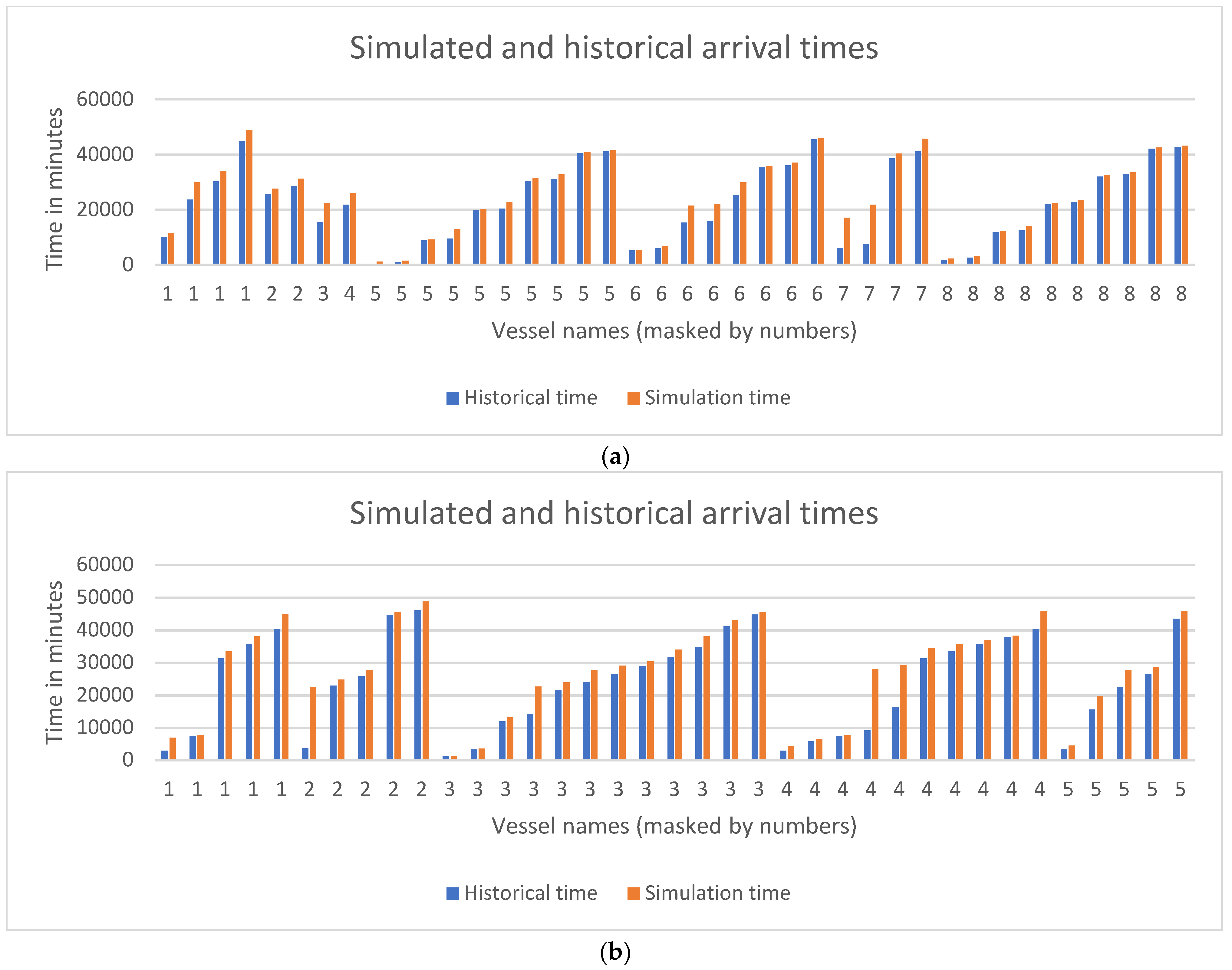
The historical data include arrival and departure times at ports along with the time spent at port. As mentioned earlier, only the port departure times are included as inputs in the model. The arrival of a vessel at its destination port depends on the ice conditions, dirways, the availability of icebreakers, and the logic of how icebreakers prioritize assistance requests from multiple vessels. One of the ways to validate the model is by comparing the arrival times of vessels at different ports in its schedule with the historical arrival times. A total of 249 trips were analyzed. For ease of visibility, a set of ships were chosen to be presented.
Figure 8a,b show the simulated and historical arrival times plotted for two sets of ships. It is observed that most trips are close to their expected arrival times. There are instances, such as Vessel 4 in
Figure 8b, where significant delays are experienced. Study of such cases will help to improve the model in future work.
8.2.4. Parameter Variability—Sensitivity Analysis
According to this method, the input parameters of the model are varied and the effects on the output behavior are noted. Firstly, a qualitative analysis is performed, where the directions of output changes are compared with those expected in the real system. The expected behavior of the real system is obtained through interviews with field experts. Next, the magnitudes of outputs are also compared. This approach is similar to the first validation approach (comparison with other models), the difference being that instead of comparing other models, the comparison is made using field experts’ descriptions of expected output behavior. The difference between face validity and parameter sensitivity is that in parameter sensitivity the various system parameters are varied one at a time and their effect on the system is observed. This helps to validate that the parameters are captured correctly and that their interaction with the system is modelled correctly as well. In face validity, overall system behavior is observed and validated. It is possible that even though face validity is successful, parameter variability sensitivity analysis may bring out inaccuracies (if any) in the modelling of specific parameters. The current model contains more parameters than the previous efforts and hence this approach allows for a complete validation study.
Table 5 shows the parameters of the simulation model along with their ranges and default values. These are vessel speed threshold (the speed below which icebreaker assistance is required), the maximum waiting time allowable for any vessel before it receives icebreaker assistance, whether convoys are being built or not (convoy mode on/off), and maximum allowable convoy size (or minimum convoy speed).
Additionally, vessel fleet size (the number of vessels in the system) is parameterized, such that it is possible to change the number of vessels for the period in order to gauge how model performance scales up with increase in the number ofvessels. Multiple parameter variation experiments have been performed. The results of the qualitative study are presented in
Table 6. The quantitative studies are described in detail in the following section.
From the validation studies, it is confirmed that the behavior of the model is aligned with the real system behavior as well as that of the previous simulation efforts. The next section presents some computational experiments with parameter variation to provide further insight into the functioning of the model.
9. Computational Experiments
The first parameter varied was the number of vessels, increased gradually from 1, 25, 50, 100, to 116 vessels in different runs.
Table 7 shows the results of varying the number of vessels in the system. As per the historical data used, all trip itineraries are completed by 15 February, with all vessels exiting the system. If all departure times are adhered to in the simulation run, then this condition will be met, and the last vessel will leave the system by 15 February. If the departure times are delayed, then the overall end time of the simulation may also go beyond 15 February.
Table 7 reports the final difference from the overall schedule as a percentage. It is calculated as shown in the equation:
The icebreakers use the Longest Waiting Time First (LWTF) criteria while selecting vessels to assist. According to this method, the requests received by icebreakers are sorted by the duration of time that has elapsed since receipt of the request. Every vessel has an attribute that keeps note of the waiting time until assistance is received. The vessel that has waited the longest is chosen to be assisted first. If LWTF is not used, it is important to define the parameter that specifies maximum allowable waiting time (
). Without this parameter, it is possible that a vessel may remain unassisted till the end of the time period for receiving assistance, while other vessels are prioritized over it. Due to
it is ensured that once the waiting time of a vessel crosses the maximum allowable time, it is immediately prioritized over all others and assisted.
The difference in scheduling begins to appear when the traffic is increased to 25 vessels or more. Although it can be observed that for the last two scenarios with higher traffic volumes there is a slightly higher difference between the observed schedules and the historical data, the output values are quite close for all the traffic situations. It can be said that system performance is nearly consistent for increasing traffic conditions. The observed difference in schedules is not unexpected since the model at this stage does not capture all the real-life decision-making actions. Firstly, convoy sizes are often larger than two and hence more vessels are assisted at once. Further, icebreakers often optimize their trips to improve overall system performance (reducing average waiting time). Icebreaker assistance mission planning is a complex problem and is beyond the scope of this article.
Next, experiments were conducted by varying the icebreaker assistance threshold (minimum speed),
. Icebreakers can decide whether to let a vessel continue its journey at a given speed or to step in and assist. In practice, the vessel speed threshold for icebreaker assistance depends on the ice and traffic situation and the availability of icebreakers. The lower the threshold, the further the vessels must travel without assistance. Consequently, the higher the threshold, the busier the icebreakers. The experiments were carried out for N = 50 and 116. The range of the icebreaker assistance threshold was from 3 to 6 kn. This threshold varied in steps of 1 kn.
From
Table 8, it can be observed that for N = 50 system performance was almost similar for all values of
. However, for N = 116 the system performance varied for higher values of
. For
, the system performed significantly worse than the other configurations. A higher value of
implies that the icebreakers need to start assisting the vessels sooner and hence are busier. This also means that vessels must wait longer for icebreakers to become available.
10. Discussion and Conclusions
This article presents a simulation-based approach for the challenging and complex winter navigation system in the Bay of Bothnia. While simulation techniques have been applied before to this problem, the novelty of this paper’s application lies in the powerful visualization and the integration of data from different sources into a unified, functional model. The model also captures varying ice conditions in detail and their impact on vessel speeds and dirways. Icebreaker assistance was modelled and the impact of adding intelligence to their decision making was studied through preliminary experiments. Furthermore, convoy situations and their related parameters were also successfully captured. The model is based on real-world historical data and inputs from field experts. The behavior of vessels and icebreakers was defined using an agent-based simulation paradigm to capture these effects. The model has been thoroughly verified and validated, both by visual inspection and by comparison with historical data. Experimental results have been presented to describe the validation process in a systematic and detailed manner. The results indicate that the model is in close agreement with the conceptual description and with the historical data. The differences with real-world data observed were as expected. The model is a successful proof of concept and provides a basis for building a simulation-based decision-support system for winter navigation. The navigation of merchant vessels in ice and their interactions with icebreakers are highly complex. Through multiple experiments, some of these complexities have been identified and studied. The interdependencies of the parameters have also been highlighted at multiple instances.
11. Future Research
This model is part of ongoing continuous work on building decision-support capabilities for winter navigation using simulation techniques. The immediate extensions of this work include increasing the operational area to the entire Baltic Sea Region. Further, longer winter periods and multiple winters will be included in the analysis. The current version introduces the concept of convoys. In the ongoing work, different types of convoys and towing situations will be addressed, including instances where two icebreakers are required at once. An important extension of this work involves exploring more details of the ice data and their incorporation into the model. Through complex expressions for equivalent ice thicknesses, more factors relating to ice conditions are being included. The icebreaker-assistance mission optimization problem is also an important part of the future work. Lastly, ship-level details are being worked on, to be included in the model. A unique combination of ship-level and system simulation is underway, allowing the impact of an individual vessel’s dimensions and icebreaking capacities on the traffic in the system to be gauged.


