Hyperspectral Estimation of Nitrogen Content in Different Leaf Positions of Wheat Using Machine Learning Models

Abstract

Remote sensing estimation of crop nitrogen content allows real-time monitoring of growth to develop scientific methods. However, most of the current remote sensing estimates of crop nitrogen contents have limitations in accurately reflecting the vertical distribution of nutrients in plants. Firstly, the original hyperspectrum is first-order differential (FD), second-order differential (SD), and continuous removal (CR), and the corresponding sensitive bands were screened by correlation analysis in this paper. Then, the spectral reflectance, vegetation indices, and wavelet coefficients were used as input features to construct models for estimating nitrogen content of flag leaf, upper 1 leaf, upper 2 leaf, upper 3 leaf, and upper 4 leaf based on partial least squares regression (PLSR), support vector machine (SVM), random forest (RF), and multiple linear regression (MLR), respectively. The results showed that the accuracy of nitrogen content prediction based on wavelet coefficients was the highest. The combination of MLR and SVM with wavelet coefficients had high accuracy and robustness in the prediction of nitrogen content at different leaf positions. Additionally, the prediction accuracy of nitrogen gradually increased as the leaf position of winter wheat increased. The study can provide technical support for remote sensing estimation of nutrient elements at vertical leaf position of crops. The study can provide a reference for prediction of other crops.

1. Introduction

Wheat is one of the most widely cultivated food crops in the world, with China ranking first in terms of its production and sales [1]. Nitrogen is the most significant nutrient for wheat growth, high grain yield, and quality [2]. Therefore, precise assessment of both nitrogen content in wheat plants is important for monitoring growth and development and early prediction of grain yield. The traditional method of estimating N content in wheat mainly relies on destructive sampling in the field and is obtained using chemical analysis. This method is inefficient, costly, and cannot obtain spatially continuous distribution of N content, which makes it difficult to meet the demand for rapid, real-time, and large area monitoring. In recent years, with the development of remote sensing technology, research and applications in crop nutrition diagnosis have been gradually promoted. Currently, most of the relevant studies on remote sensing estimation of crop phenotypic parameters are based on the canopy scale. The study showed that both the spectral reflectance of crop canopy and its derivative spectra were highly correlated with N content, which proved the feasibility of using spectral reflectance to estimate the N content of crops [3]. This indicates that spectral information is a good non-destructive surrogate to the above crop traits. Han et al. [4] have reported a significant influence of changes in center wavelength, band density, and signal-to-noise ratio, and sensitivity and effectiveness of spectral indices in assessing the chlorophyll content. Some studies have also applied principal component analysis to extract and reduce the dimension of the original spectral data and used support vector machine (SVM) and multiple linear regression (MLR) algorithms to predict leaf nitrogen content in citrus and other fruit trees [5,6].

During the growth of winter wheat, the population exhibits different canopy spatial structures, and there are characteristics of vertical distribution of nitrogen in the crop and corresponding changes in chlorophyll, etc., in the middle and lower leaves of winter wheat as the reproductive period progresses [7]. Therefore, the study of vertical heterogeneity of biochemical parameters of winter wheat leaves is important for monitoring various growth conditions such as the growth potential of winter wheat. Previously, some studies have reported the vertical estimation of nitrogen and chlorophyll level using hyperspectral information at different leaf positions in wheat. Dang et al. [8] have studied the vertical distribution of nitrogen and chlorophyll in winter wheat leaves under different nitrogen application levels through field experiments. Luo et al. [9] showed that there were differences in nitrogen and chlorophyll in cotton leaves in various leaf positions. The above results demonstrated that increment in nitrogen fertilizer application rate could enhance nitrogen content across the leaves for better photosynthesis activity in plants [10]. However, most of the existing studies mainly focus on the estimation of nitrogen in crop canopy, as well as the difference patterns and spectral characteristics of nitrogen distribution in different leaf positions. To our knowledge, there are few studies using remote sensing technology to monitor the growth parameters of crops at different leaf positions.

The main objectives of this study are as follows: (1) to analyze the differences in spectral variation characteristics of physiological parameters at different leaf positions in winter wheat; (2) to evaluate the ability of spectral reflectance, vegetation index, and wavelet transform coefficients for estimating N content at different leaf positions; and (3) to screen optimal estimation models for N content at different leaf positions based on four machine learning algorithms. This paper can provide theoretical and technical references for studying the vertical variation characteristics of other crop growth parameters using remote sensing technology.

2. Materials and Methods

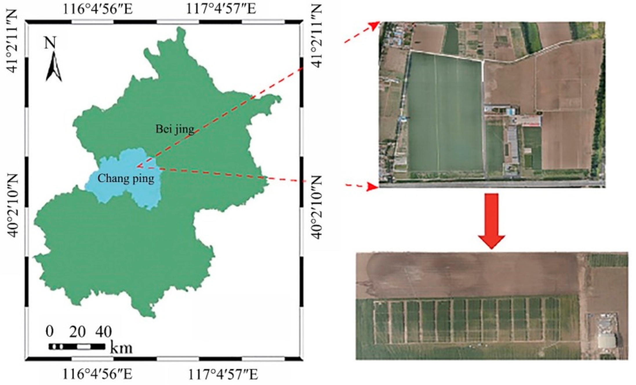
2.1. Experiment Location and Research Material

The study was conducted in the Chang Ping District, Beijing (Figure 1). The base is flat and fertile. The mass fractions of nitrate nitrogen, quickly available potassium, and available phosphorus in 0–0.3 m soil layer of the experimental field were 3.16–14.82, 86.83–120.62, and 3.14–21.18 mg·kg⁻¹, respectively. The soil organic matter content was 15.8–20.0 g·kg⁻¹. Its average elevation is approximately 36 m, and the soil type is tidal soil. The average annual temperature is approximately 13 °C. The average annual rainfall is approximately 510 mm. In order to increase the difference in crop nitrogen content in each experimental plot, the study was carried out by using two types of wheat: Zhong Mai 175 and the Jing 9843 type. Four different nitrogen levels were set up for nitrogen treatment: N1: 0 kg·hm⁻²; N2: 195 kg·hm⁻²; N3: 390 kg·hm⁻²; and N4: 585 kg·hm⁻². The nitrogen fertilizer was urea. Base and elongation fertilizers were applied to the soil at 1/2 of the total amount of fertilizer applied. Wheat planting was undertaken on 29 September 2017. The size of each experimental plot was 1.2 × 1.5 m, with 16 plots and 3 replications, totaling 48 plots.

2.2. Data Collection and Processing

The spectra of wheat leaves from different layers were measured using ASDFieldSpec FR2500 (spectral range 350–2500 nm, interval 1 nm, Malvern Panalytical, Westborough, MA, USA). During measurement of the spectral data, the probe height was maintained at 40 cm away from the leaf with field of view of 25°. Ten spectral curves of each sample were measured and processed using ViewSpecPro software (https://www.xiazaila.com/soft/26270.html, accessed on 7 June 2022, V5.6.8, China) to obtain the dimensionless reflectance.

Three samples of wheat plants with uniform growth were randomly selected in the experimental plot and quickly brought back to the laboratory in fresh bags. Then, each layer of leaves was separated and the nitrogen content of the leaves was measured using the Kjeldahl method.

2.3. Method

2.3.1. Continuous Wavelet Transform

Continuous wavelet transform (CWT) is a linear transformation method that decomposes hyperspectral data into a series of wavelet coefficients with different scales by using wavelet basis functions [11]. The transformation formula is (Equation (1)):

$$f(a,b)={\displaystyle {\int }_{-\infty }^{+\infty }f(\lambda )}{\phi }_{a,b}(\lambda )d\lambda$$

(1)

where $f(\lambda )$ is the spectral reflectance, $\lambda$ is the spectral band in the range of 350–2500 nm, ${\phi }_{a,b}$ is the wavelet basis function, a is the scale factor, and b is the translation factor. In this study, a Meyer function with fast convergence speed was selected as the wavelet basis function, and CWT was performed based on MATLAB software (MATLAB 2021, MathWorks Company, Natick, MA, USA). In order to reduce the redundancy of data, the scale of the continuous wavelet transform was decomposed into 21, 22, 23, …, 210, corresponding to scale 1, 2, 3, …, 10.

2.3.2. Spectral Differential Transformation

The Grünwald–Letnikov differential form was used to differentiate the hyperspectral data [12]. The form is as follows (Equation (2)):

$$\frac{d^{a}f(\lambda )}{d{\lambda }^a}\approx f(\lambda )+(-a)f(\lambda -1)+\frac{(-a)(-a+1)}{2}f(\lambda -2)+\cdots +\frac{\Gamma (-a+1)}{n!\Gamma (-a+1)}f(\lambda -n)$$

(2)

where $\Gamma$ represents the Gamma function, $\lambda$ represents the corresponding wavelength, n represents the difference between the upper and lower limits of the differential, and α represents any order. When α = 0, 1, and 2, it indicates the original spectrum, the FD spectrum, and the SD spectrum, respectively.

2.3.3. Construction of Vegetation Indices

Many studies have shown that vegetation indices can improve vegetation information and are widely used for crop monitoring. In this study, 20 vegetation indices [13,14,15] were screened for estimating the nitrogen content levels in different leaf positions of wheat. The formulas are shown in

Table 1. Description of vegetation indices.

Name	Formula
Normalized Difference Vegetation Index (NDVI)	(Rnir − Rred)/(Rnir + Rred)
Ratio Vegetation Index (RVI)	Rnir/Rred
Difference Vegetation Index (DVI)	Rnir-Rred
Optimized Soil-Adjusted Vegetation Index (OSAVI)	1.16 × (Rnir − Rred)/(Rnir + Rred + 0.16)
Optimal Vegetation Index (VIOPT)	1.45 × (RniR2 + 1) × (Rred + 0.45)
Normalized Difference Water Index (NDWI)	(R860 − R1240)/(R860 + R1240)
Water Index (WI)	R900/R970
Transformed Chlorophyll Absorption Ratio (TCARI)	3× ((R700 − R670) − 0.2 × (R700 − R550) × (R700/R670))
Chlorophyll Index Red Edge (CI red edge)	(Rnir/Rred edge) − 1
Red-Green Vegetation Index (RGVI)	Rred/Rgreen
Red-Blue Vegetation Index (RBVI)	Rred/Rblue
Green-Blue Vegetation Index (GBVI)	Rgreen/Rblue
Misra Green-Red Vegetation Index (MGRVI)	(R2green − R2red)/(R2green + R2red)
Relative Green-Blue Vegetation Index (RGBVI)	(R2green − Rblue × Rred)/(R2green +Rblue × Rred)
Green Leaf Area (GLA)	(2 × Rgreen – Rred − Rblue)/(2 × Rgreen + Rred − Rblue)
Excess Red (EXR)	1.4 × Rred − Rgreen
Excess Green (EXG)	2 × Rgreen – Rred − Rblue
Excess Green Minus Excess Red (EXGR)	2 × (Rgreen – Rred − Rblue) − 1.4 × (Rred + green)
Color Index of Vegetation (CIVE)	0.441 × Rred − 0.881 × Rgreen + 0.3856 × Rblue + 18.79
Visible Atmospherically Resistant Indices (VARI)	(Rgreen − Rred)/(Rgreen + Rred − Rblue)

Note: R represents the spectral reflectance of the band.

.

2.3.4. Machine Learning Methods

Partial least-square regression (PLSR) is a data modeling method that draws on concepts from multiple linear regression analysis, canonical correlation analysis, and principal component analysis. This method focuses on the linear relationship between the independent and dependent variables, and hence can solve the multicollinearity problem and guarantee model stability [16].

Support vector machines (SVMs) [17] can find the optimal hyperplane which can maximally separate multidimensional samples of two different classes. For two-dimensional and three-dimensional sample spaces, the optimal hyperplane is a straight line and a plane, respectively, while for the higher dimensional n-dimensional sample space, the optimal hyperplane is abstractly defined as an (n − 1)-dimensional space. For linearly separable problems, finding the optimal hyperplane can be transformed into solving a quadratic programming problem. For nonlinearly separable problems, the kernel trick can be applied to project the input features into a higher dimensional space where the problem becomes linearly separable.

Random forests (RF) use random resampling to generate multiple sample sets from the original sample set. A tree classifier is generated based on each sample set, and then the final classification output is made according to an ensemble of multiple tree classifiers. Each sample set is used to train a single classification tree [18]. At the nodes of the tree, M features are randomly selected from m features (where m > M). According to the minimum node impurity principle, one of the m features is selected for branch growth, and the tree is grown to minimize the impurity of each node.

Multiple linear regression (MLR) is a statistical regression method, with advantages of simplicity, low computational complexity, and high fitting accuracy [19]. Assuming that the dependent random variable y is affected by k independent variables $x_1,x_2,\cdots ,x_{\mathrm{k}}$, it can be expressed as (Equation (3)):

$$y={\beta }_0+{\beta }_1{x}_1+{\beta }_2{x}_2+\cdots +{\beta }_{\mathrm{k}}{x}_{\mathrm{k}}+\epsilon$$

(3)

where ${\beta }_0,{\beta }_1,{\beta }_2,\cdots ,{\beta }_{\mathrm{k}}$ are the model regression coefficients and $\epsilon$ is a random error. The regression coefficient can be obtained using the least-square method.

2.3.5. Correlation Analysis

Correlation analysis was completed to estimate the correlations between hyperspectral traits and nitrogen and chlorophyll contents. The calculation method is as shown in formula (Equation (4)):

$${\rho }_{X,Y}=\frac{\mathrm{cov}(X,Y)}{{\sigma }_X{\sigma }_Y}=\frac{E(XY)-E(X)E(Y)}{\sqrt{E(X^2)-E^2(X)}\sqrt{E(Y^2)-E^2(Y)}}$$

(4)

where ${\rho }_{X,Y}$ represents the correlation coefficient and $\mathrm{cov}(X,Y)$ and $\sigma$ represent the covariance and standard deviation, respectively.

2.3.6. Model Accuracy Evaluation Indicators

The coefficient of determination (R²), root mean squared error (RMSE), and normalized root mean squared error (nRMSE) were selected as the model accuracy evaluation indicators. The calculation methods are as shown in formulas (Equations (5)–(7)).

$$R^2=\frac{({\displaystyle {\sum }_{i=1}^n{y}_i-\overline{y}{)}^2}}{({\displaystyle {\sum }_{i=1}^n{x}_i-\overline{y}{)}^2}}$$

(5)

$$\mathrm{RMSE}=\sqrt{\frac{{\displaystyle {\sum }_{i=1,j=1}^n{(x_i-y_i)}^2}}{n}}$$

(6)

$$\mathrm{nRMSE}=\sqrt{\frac{{\displaystyle {\sum }_{i=1,j=1}^n{(x_i-y_j)}^2}}{n}}/\overline{y}$$

(7)

where $x_i$ is the measured value; $y_i$ is the estimated value; $\overline{y}$ is the mean value; and $n$ is the number of samples.

3. Results

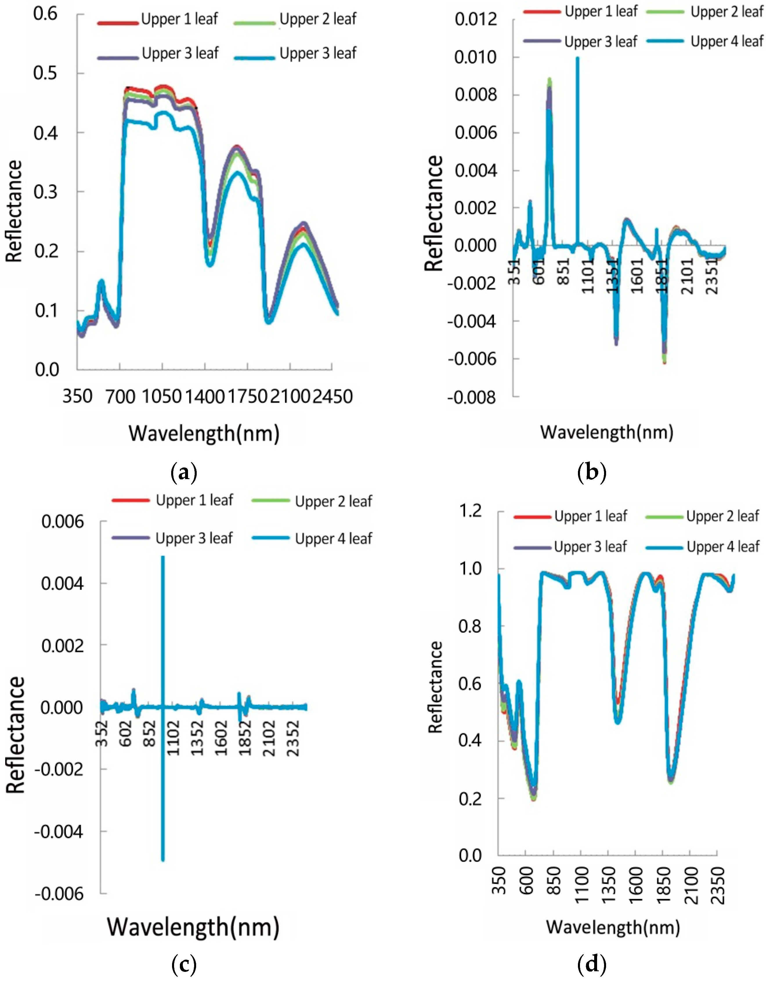
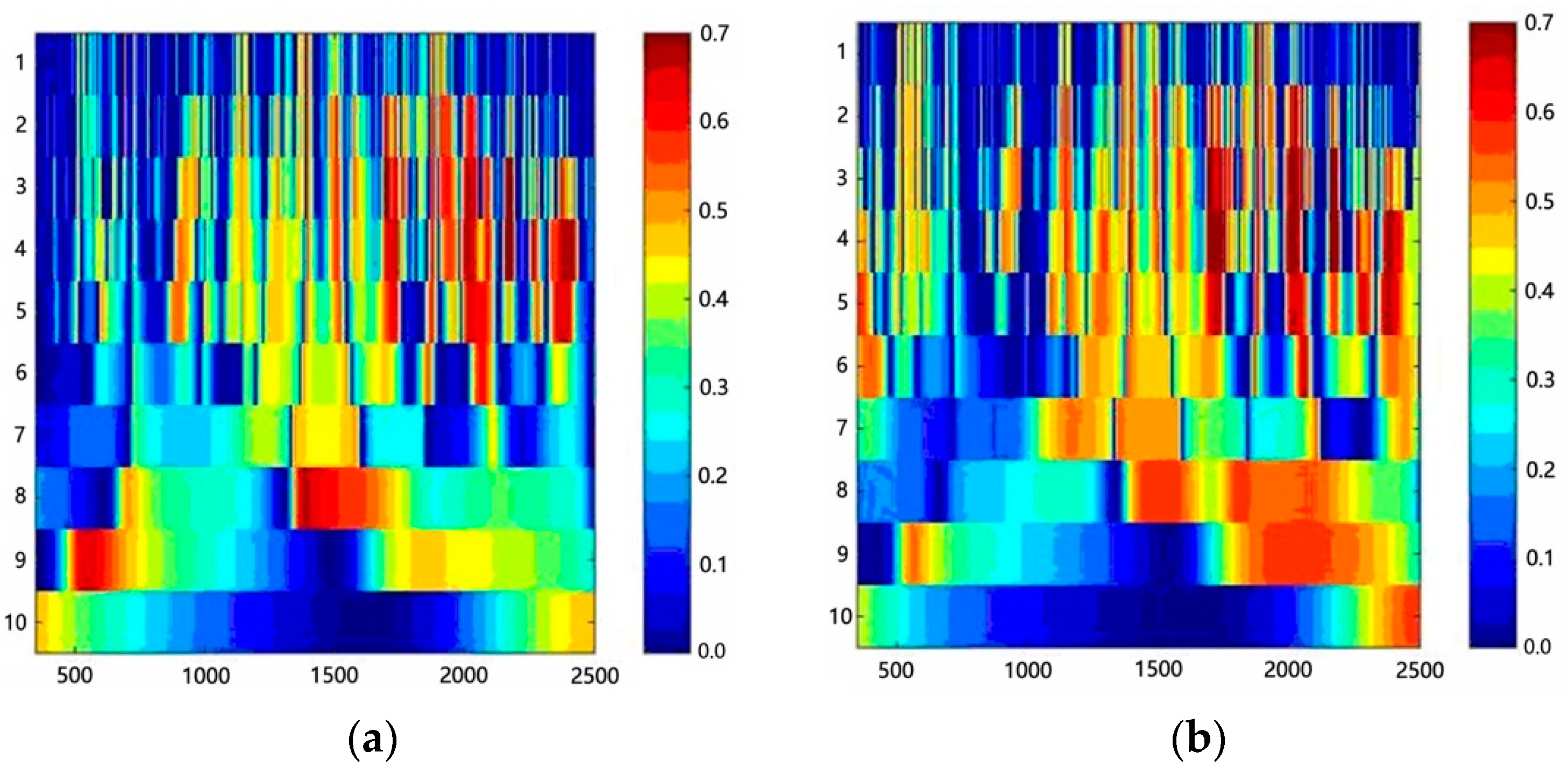
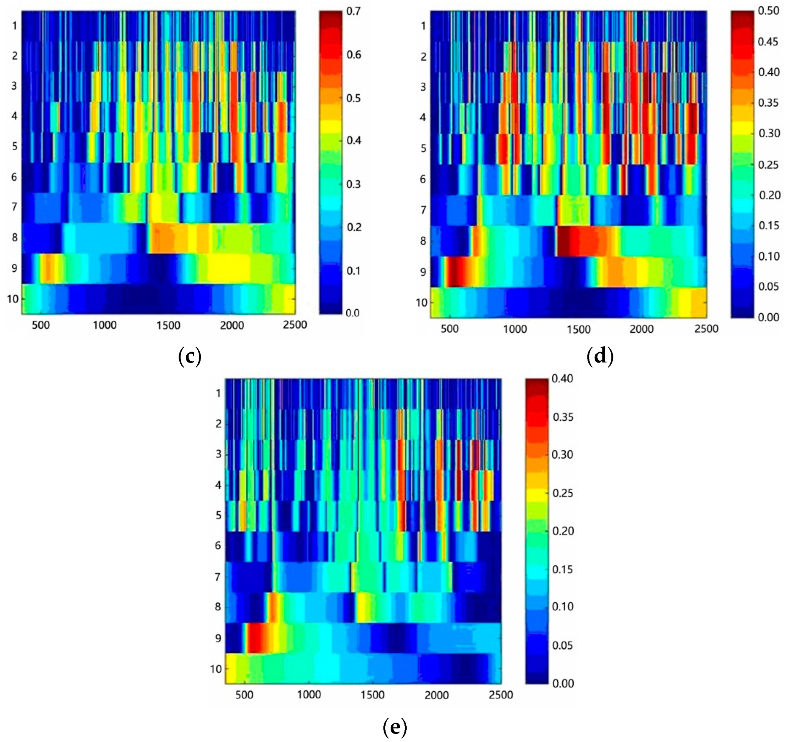
3.1. Spectral Response Characteristics of Wheat Leaves at Different Positions

The original spectra were processed using first-order differential, second-order differential, and continuous removal methods, and the spectral curves were plotted for different positions of different leaves. Figure 2 showed the spectral curves of one of the key growth periods (flag-raising stage).

There are differences in the original spectral reflectance of leaves at different leaf positions. The spectral reflectance of leaves increased with the increased number of leaf positions, and was obviously different between 750–1300 nm and 1400–1900 nm. In other band ranges, the spectral reflectance of leaves at different positions was similar. The reflectivity of FD of leaves at different leaf positions showed no difference, and there was a clear reflection peak near 743 nm. There was no difference in reflectivity of SD of leaves at different leaf positions. The SD fluctuated in the range of 550–1000 nm and 1700–1950 nm, with the maximum value near 940 nm. There was no difference in reflectance of the CR spectrum of different leaf positions; the reflectance was peaked in the visible–near infrared region of 750–1300 nm.

3.2. Construction of Nitrogen Content Model Based on the Spectral Reflectance

The original spectra of different leaf positions of winter wheat were FD, SD, and CR transformed. The correlation between spectral reflectance and nitrogen content of leaves at different leaf positions was analyzed, and the bands with strong correlations were selected as sensitive bands, and the results are shown in

Table 2. Correlation analysis of different transform spectra and leaf nitrogen content in different leaf positions and the results of screening sensitive bands.

Sort	Flag Leaf		Upper 1 Leaf		Upper 2 Leaf		Upper 3 Leaf		Upper 4 Leaf
	$\left(\mathit{\lambda }\right)$	$\left|\mathit{r}\right|$	$\left(\mathit{\lambda }\right)$	$\left|\mathit{r}\right|$	$\left(\mathit{\lambda }\right)$	$\left|\mathit{r}\right|$	$\left(\mathit{\lambda }\right)$	$\left|\mathit{r}\right|$	$\left(\mathit{\lambda }\right)$	$\left|\mathit{r}\right|$
1	FD (649)	0.89	FD (929)	0.84	FD (1232)	0.76	FD (727)	0.75	FD (1421)	0.67
2	FD (659)	0.89	FD (950)	0.82	FD (1234)	0.76	FD (621)	0.74	FD (1610)	0.59
3	SD (685)	0.89	FD (926)	0.83	FD (1229)	0.75	SD (543)	0.74	FD (1418)	0.59
4	SD (748)	0.88	FD (927)	0.83	FD (1233)	0.74	SD (589)	0.73	FD (1598)	0.57
5	SD (780)	0.87	SD (925)	0.83	FD (1231)	0.74	SD (542)	0.73	FD (1618)	0.57

Note: the $\left|r\right|$ represents the absolute value of the correlation coefficient and the $\lambda$ indicates the band position.

.

Overall, the correlation between nitrogen content and transformed spectra increased with leaf position, with high correlation in leaves of all positions. The sensitive bands of the flag leaf were concentrated in the visible light–near infrared bands between the 640–790 nm band. The spectral bands with the highest correlation (|r| = 0.89) with flag leaf nitrogen content were FD (649), FD (659), and SD (685). The sensitive bands of the upper 1 leaf were concentrated in the near–infrared bands of the FD and SD between 900 and 1000 nm. The spectral band with the highest correlation (|r| = 0.84) with the nitrogen content of the upper 1 leaf was FD (929). The sensitive bands of the upper 2 leaf were concentrated in the FD near–infrared bands between 1200 and 1250 nm. The spectral bands with the highest correlation (|r| = 0.76) with the nitrogen content of the upper 2 leaf were FD (1232) and FD (1234). The sensitive bands of the upper 3 leaf were concentrated in the visible light bands with the FD and SD between 540 and 730 nm. The spectral band with the highest correlation (|r| = 0.75) with the nitrogen content of the upper 3 leaf was FD (727). The sensitive bands of the upper 4 leaf were concentrated in the mid-infrared bands of the FD, between 1400 and 1620 nm. The spectral band with the highest correlation (|r| = 0.67) with the nitrogen content of the upper 4 leaf was FD (1421).

Using the spectral sensitive bands selected in Table 2, the prediction models of leaf nitrogen content at different leaf positions of wheat were constructed based on PLSR, SVM, RF, and MLR, respectively. In this study, the nitrogen content estimation models were established using 2/3 of the sample data, and the accuracy of the models was validated using the remaining 1/3 of sample data, and the results are shown in

Table 3. Model accuracy of estimating leaf nitrogen content based on sensitive bands.

Leaf Position	Model	Modeling Accuracy			Verification Accuracy
		R2	RMSE	NRMSE	R2	RMSE	NRMSE
Flag leaf	PLSR	0.61 **	0.08	0.06	0.58 **	0.19	0.14
	SVM	0.47 **	0.09	0.08	0.42	0.23	0.21
	RF	0.26 **	0.12	0.09	0.23	0.22	0.16
	MLR	0.55 **	0.08	0.06	0.55 **	0.19	0.13
Upper 1 leaf	PLSR	0.47 **	0.16	0.09	0.55 **	0.16	0.09
	SVM	0.37 **	0.16	0.18	0.36	0.20	0.22
	RF	0.28 **	0.18	0.11	0.30 *	0.20	0.12
	MLR	0.55 **	0.14	0.08	0.57 **	0.16	0.10
Upper 2 leaf	PLSR	0.43 **	0.09	0.08	0.52 **	0.11	0.09
	SVM	0.32 **	0.10	0.20	0.35	0.11	0.21
	RF	0.32 **	0.10	0.08	0.38 *	0.11	0.09
	MLR	0.39 **	0.09	0.08	0.47 **	0.11	0.10
Upper 3 leaf	PLSR	0.13 **	0.13	0.12	0.11	0.13	0.12
	SVM	0.42 **	0.13	0.22	0.45 **	0.15	0.26
	RF	0.12	0.10	0.10	0.21	0.16	0.14
	MLR	0.15 *	0.13	0.12	0.17	0.12	0.11
Upper 4 leaf	PLSR	0.17 *	0.11	0.14	0.20	0.14	0.18
	SVM	0.40 **	0.12	0.19	0.42 **	0.13	0.20
	RF	0.11	0.11	0.14	0.15	0.15	0.18
	MLR	0.17 *	0.09	0.11	0.14	0.14	0.18

Note: * indicates a significant correlation at the 0.05 level and ** indicates a significant correlation at the 0.01 level.

.

The results showed that the best model for nitrogen content estimation for flag leaves was PLSR with 0.61 and 0.58 R² values for modeling and validation. The optimal model for the upper 1 leaf was MLR with R² values 0.55 and 0.57 for modeling and validation. The PLSR was the best model for the upper 2 leaf with R² values 0.43 and 0.52 for modeling and validation. The optimal model for the upper 3 leaf was SVM with 0.42 and 0.45 R² values for modeling and validation. The optimal model for nitrogen content estimation in the upper 4 leaf was SVM with R² values for modeling and validation of 0.40 and 0.42, respectively.

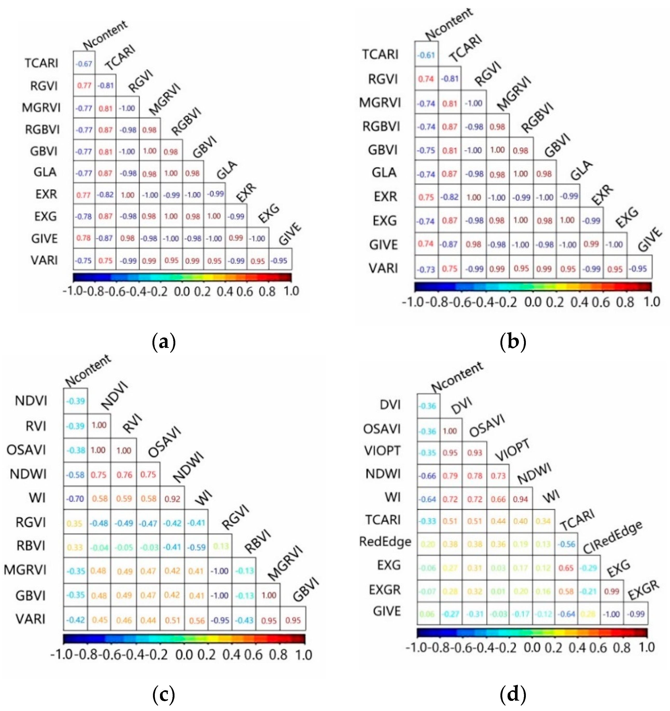
3.3. Construction of the Nitrogen Content Model Based on Vegetation Indices

The correlation analysis between vegetation indices constructed in Table 1 and leaf nitrogen content at different leaf positions was carried out, and the correlation coefficient matrices were drawn. The results are shown in Figure 3.

Based on the results of the correlation analysis between the nitrogen content of leaves at different leaf positions and vegetation indices, the vegetation indices with high correlation were screened and the results are shown in

Table 4. Correlation between vegetation indices and nitrogen content from different leaf positions in winter wheat.

Sort	Flag Leaf		Upper 1 Leaf		Upper 2 Leaf		Upper 3 Leaf		Upper 4 Leaf
	$\left(\mathit{\lambda }\right)$	$\left|\mathit{r}\right|$	$\left(\mathit{\lambda }\right)$	$\left|\mathit{r}\right|$	$\left(\mathit{\lambda }\right)$	$\left|\mathit{r}\right|$	$\left(\mathit{\lambda }\right)$	$\left|\mathit{r}\right|$	$\left(\mathit{\lambda }\right)$	$\left|\mathit{r}\right|$
1	EXR (red green)	0.78	GBVI (green blue)	0.75	WI (900 970)	0.70	NDWI (860 1240)	0.66	TCARI (700 670 550)	0.48
2	GLA (red green blue)	0.78	MGRVI (green red)	0.74	NDWI (860 1240)	0.58	WI (900 970)	0.64	GIVE (red green blue)	0.47
3	RGBVI (red green blue)	0.77	RGVI (red green)	0.74	NDVI (nir red)	0.39	VIOPT (nir red)	0.35	VIOPT (nir red)	0.44
4	GBVI (green red)	0.77	GLA (green blue red)	0.74	OSAVI (nir red)	0.38	DVI (nir red)	0.36	WI (900 970)	0.37
5	MGRVI (green red)	0.77	EXR (red green)	0.74	RVI (nir red)	0.39	TCARI (670 700)	0.33	Red Edge	0.36

Note: $\left|r\right|$ represents the absolute value of the correlation coefficient and $\lambda$ indicates the band position.

.

The results showed that the correlations between the nitrogen content of leaves at different leaf positions and vegetation indices improved with increasing leaf positions. The vegetation indexes with the highest correlation with the nitrogen content of flag leaf were EXR and GLA (|r| = 0.78). The vegetation indices with the highest correlation with nitrogen content at different leaf positions in the upper 1, upper 2, upper 3, and upper 4 were GBVI, WI, NDWI, and TCARI (|r| = 0.75, 0.70, 0.66, and 0.48), respectively.

Based on the results of correlation analysis between leaf nitrogen content and vegetation indices, the top five vegetation indices with high correlation at different leaf positions were screened for model construction, and the results are shown in

Table 5. Model accuracy of estimating nitrogen content based on vegetation indices.

Leaf Position	Model	Modeling Accuracy			Verification Accuracy
		R2	RMSE	NRMSE	R2	RMSE	NRMSE
Flag leaf	PLSR	0.68 **	0.07	0.06	0.58 **	0.10	0.09
	SVM	0.51 **	0.08	0.16	0.58 **	0.12	0.22
	RF	0.49 **	009	0.07	0.45 **	0.12	0.10
	MLR	0.64 **	0.08	0.06	0.54 **	0.09	0.08
Upper 1 leaf	PLSR	0.60 **	0.14	0.08	0.57 **	0.18	0.11
	SVM	0.59 **	0.13	0.15	0.52 **	0.17	0.19
	RF	0.45 **	0.15	0.09	0.43 **	0.19	0.11
	MLR	0.55 **	0.13	0.08	0.51 **	0.17	0.10
Upper 2 leaf	PLSR	0.33 **	0.16	0.12	0.28 *	0.12	0.09
	SVM	0.53 **	0.09	0.08	0.49 **	0.21	0.19
	RF	0.38 **	0.10	0.07	0.48 **	0.23	0.17
	MLR	0.54 **	0.14	0.10	0.53 **	0.11	0.09
Upper 3 leaf	PLSR	0.44 **	0.10	0.10	0.52 **	0.10	0.10
	SVM	0.42 **	0.11	0.16	0.32 *	0.13	0.22
	RF	0.24 **	0.10	0.10	0.44 **	0.15	0.14
	MLR	0.50 **	0.09	0.08	0.52 **	0.11	0.11
Upper 4 leaf	PLSR	0.31 **	0.08	0.10	0.28 *	0.13	0.17
	SVM	0.33 **	0.10	0.16	0.31 *	0.11	0.16
	RF	0.16 *	0.10	0.12	0.12	0.13	0.16
	MLR	0.37 **	0.08	0.10	0.35 *	0.13	0.16

Note: * indicates a significant correlation at the 0.05 level and ** indicates a significant correlation at the 0.01 level.

.

Overall, the accuracy of leaf nitrogen content estimation gradually improved with the increase in leaf position. The results showed that the best model for flag leaf nitrogen content estimation was PLSR with modeling and validation R² of 0.68 and 0.58; the best model for upper 1 nitrogen content estimation was PLSR with modeling and validation R² of 0.60 and 0.57; the optimal model for upper 2 nitrogen content estimation was MLR with modeling and validation R² of 0.54 and 0.53; the highest accuracy model for upper 3 nitrogen content estimation was MLR with modeling and validation R² of 0.50 and 0.52; the optimal model for upper 4 nitrogen content estimation was MLR with modeling and validation R² of 0.37 and 0.35, respectively.

3.4. Construction of the Nitrogen Content Model Based on the Wavelet Coefficients

The original spectral reflectance was converted into wavelet coefficients corresponding to 10 scales using CWT. Sensitivity analysis was conducted on the wavelet coefficient and nitrogen content of leaves at different leaf positions, and the correlation matrix diagrams were drawn. The results are shown in Figure 4.

Based on the wavelet coefficients obtained by the CWT, the sensitive wavelet energy coefficients were screened, and the results are shown in

Table 6. Correlations of different leaf position wavelet coefficients and leaf nitrogen content in winter wheat.

Sort	Flag Leaf		Upper 1 Leaf		Upper 2 Leaf		Upper 3 Leaf		Upper 4 Leaf
	$\left(\mathit{\lambda }\right)$	$\left|\mathit{r}\right|$	$\left(\mathit{\lambda }\right)$	$\left|\mathit{r}\right|$	$\left(\mathit{\lambda }\right)$	$\left|\mathit{r}\right|$	$\left(\mathit{\lambda }\right)$	$\left|\mathit{r}\right|$	$\left(\mathit{\lambda }\right)$	$\left|\mathit{r}\right|$
1	C4 (2173)	0.87	C3 (1701)	0.87	C3 (1695)	0.79	C8 (1367)	0.76	C5 (1745)	0.63
2	C4 (2172)	0.87	C3 (1703)	0.87	C3 (1694)	0.79	C8 (1366)	0.76	C5 (1746)	0.63
3	C4 (2174)	0.87	C3 (1700)	0.87	C3 (1696)	0.78	C8 (1370)	0.76	C5 (1744)	0.63
4	C4 (2171)	0.87	C3 (1704)	0.87	C3 (1693)	0.78	C8 (1369)	0.76	C5 (1747)	0.63
5	C4 (2175)	0.87	C3 (2168)	0.87	C3 (1697)	0.78	C8 (1368)	0.76	C5 (1743)	0.63

Note: $\left|r\right|$ represents the absolute value of the correlation coefficient and the $\lambda$ in the bracket represents the number of bands.

.

The overall correlations between leaf nitrogen content and wavelet coefficients at different leaf positions improved with the increasing leaf positions. The correlations between the nitrogen content of the flag leaf and upper 1 leaf were the highest, with the correlation coefficient up to 0.87, but the corresponding wavelet transform scale differed. For the band range of 1500–2500 nm, the flag leaf had the highest global sensitivity index and the corresponding scales were 3, 4, 5, 8, and 9. The coefficient with the highest correlation between the nitrogen content of the flag leaf and the wavelet coefficient was concentrated in the band between 2170 and 2180 nm with a correlation coefficient of 0.87 and the corresponding scale of 4. The global sensitivity index of the flag leaf was the highest in the band range between 1500 and 2500 nm, and the corresponding scales were 2, 3, 4, 5, and 6. The coefficient with the highest correlation between the nitrogen content of the upper 1 leaf and wavelet coefficient was concentrated between the 1700–2200 nm band, while the correlation coefficient was 0.87, and the corresponding scale was 3. The global sensitivity index of the upper 2 leaf was the highest between the 1500–2000 nm band range, and the corresponding scales were 3, 4, and 5. The coefficient with the highest correlation between the nitrogen content of the upper 2 leaf and wavelet coefficient was concentrated between the 1690–1700 nm band, with the correlation coefficient of 0.79, while the corresponding scale was 3. The band range between 1300 and 2500 nm showed best global sensitivity index for the upper 3 leaf with corresponding scales 3, 4, and 8. The positions of the wavelet coefficients with the highest correlation between the nitrogen content and wavelet coefficients in the upper 3 leaves were mainly concentrated in 1360~1370 nm, with a correlation coefficient of 0.76 and a corresponding scale of 8. The global sensitivity index of the upper 4 leaf was highest between the 1700–2500 nm band range, and the corresponding scales were 3, 4, 5, and 9. The correlation between the nitrogen content of the upper 4 leaf and the wavelet coefficient was concentrated between the 1740–1750 nm band, with a correlation coefficient of 0.63 and a corresponding scale of 5.

Based on the screened sensitive wavelet coefficients, PLSR, SVM, RF, and MLR methods were used to construct models for the estimation of leaf nitrogen content at different leaf positions and to validate the model accuracy, and the results are shown in

Table 7. Model accuracy of estimating nitrogen content based on sensitive wavelet.

Leaf Position	Model	Modeling Accuracy			Verification Accuracy
		R2	RMSE	NRMSE	R2	RMSE	NRMSE
Flag leaf	PLSR	0.79 **	0.06	0.05	0.71 **	0.08	0.07
	SVM	0.66 **	0.07	0.14	0.65 **	0.05	0.10
	RF	0.74 **	0.06	0.04	0.65 **	0.09	0.08
	MLR	0.84 **	0.06	0.05	0.89 **	0.07	0.06
Upper 1 leaf	PLSR	0.76 **	0.10	0.06	0.79 **	0.11	0.06
	SVM	0.74 **	0.08	0.09	0.78	0.12	0.13
	RF	0.72 **	0.13	0.08	0.64 **	0.09	0.05
	MLR	0.77 **	0.12	0.07	0.80 **	0.08	0.05
Upper 2 leaf	PLSR	0.60 **	0.13	0.10	0.78 **	0.08	0.06
	SVM	0.67 **	0.07	0.06	0.42 **	0.19	0.17
	RF	0.64 **	0.07	0.05	0.59 *	0.18	0.13
	MLR	0.73 **	0.12	0.09	0.74 **	0.09	0.07
Upper 3 leaf	PLSR	0.53 **	0.10	0.09	0.70 **	0.07	0.07
	SVM	0.52 **	0.09	0.15	0.50 **	0.08	0.14
	RF	0.54 **	0.09	0.08	0.47 **	0.11	0.10
	MLR	0.58 **	0.09	0.08	0.73 **	0.09	0.09
Upper 4 leaf	PLSR	0.33 **	0.10	0.13	0.55 **	0.07	0.09
	SVM	0.29 **	0.10	0.16	0.42 **	0.08	0.12
	RF	0.47 **	0.09	0.11	0.35 *	0.14	0.17
	MLR	0.51 **	0.06	0.08	0.57 **	0.07	0.09

Note: * indicates a significant correlation at the 0.05 level and ** indicates a significant correlation at the 0.01 level.

.

Overall, the accuracy of estimation of leaf nitrogen was improved with the increasing leaf positions. The results showed that the best model for estimating the nitrogen content of flag leaf was MLR with modeling and validation R² of 0.84 and 0.89, respectively. The best model for upper 1 leaf nitrogen content estimation was SVM with modeling and validation R² of 0.74 and 0.78, respectively. The best model for the upper 2 leaf nitrogen content estimation was MLR with the modeling and validation R² of 0.73 and 0.74, respectively. The best model for nitrogen content estimation in the upper 3 leaf was MLR with modeling and validation R² of 0.58 and 0.73, respectively; the best model for nitrogen content estimation in the upper 4 leaf was MLR with modeling and validation R² of 0.51 and 0.57, respectively.

4. Discussion

Nowadays, the development of remote sensing technology has provided an effective way to obtain crop phenotype information in a large area and quickly without loss, and the use of remote sensing technology to monitor the changes in crop phenotype parameters is the future development trend. In this study, the quantitative inversion of the vertical distribution of nitrogen content based on the remote sensing platform was carried out from the demand of nitrogen content monitoring. It was found that the correlation between spectral reflectance and nitrogen content of different leaf positions was significantly enhanced after FD and SD processing of the original spectrum, and the correlation coefficients could reach up to 0.89. This was mainly because the spectral information is affected by atmospheric effects and environmental factors during hyperspectral data acquisition, resulting in noise interference in the original spectrum, which can affect the extraction of sensitive information. Spectral differentiation technology could partially eliminate the influence of atmospheric effects and environmental factors, reflecting the nature of vegetation characteristics, which is consistent with the previous conclusions of Li et al. [20].

In recent years, wavelet transform, as an emerging discipline applied in remote sensing science, is one of the very promising techniques in hyperspectral information extraction, and reflects more and more advantages in data dimensionality reduction, crop identification, and inversion of crop physical and chemical parameters [21]. Our study obtained the highest prediction accuracy by constructing a nitrogen content prediction model using wavelet coefficients. This was because wavelet variations can extract the weak information hidden in the spectral signal and effectively use the overall structural characteristics of the spectral information.

It has been found that nitrogen is easily transported within the plant, resulting in significant differences in the nitrogen content of leaves at different leaf positions [22]. Therefore, studying the vertical distribution of nitrogen content within the plant is of great significance for growth monitoring, making fertilization decisions, guiding agricultural production, and monitoring pests and diseases. In this study, nitrogen content prediction models for different leaf positions were constructed based on machine learning algorithms, and all of them obtained high prediction accuracy. Among them, the flag leaf and the upper 1 leaf showed higher prediction accuracy, and MLR and SVM showed better overall prediction performance. The results can be ascribed to the fact that the upper leaves contribute the most to the canopy spectra, and as the leaf position decreases, the corresponding contribution to the canopy spectra gradually decreases. This conclusion is highly consistent with that of Xiao [23]. Machine learning has been widely used in the field of remote sensing in recent years, and our study successfully constructed nitrogen content inversion models using four algorithms, all of which achieved high prediction accuracy. However, due to the small amount of sample data used in the paper, the model may be overfitted when modeling using machine learning methods, so further increase in sample data is needed to improve the robustness of the model. The research results can provide reference for other crops in field phenotype research.

5. Conclusions

The paper used hyperspectral reflectance and nitrogen content data of winter wheat leaves to construct leaf nitrogen content prediction models for different leaf positions based on PLSR, SVM, RF, and MLR algorithms, respectively. Our study found that the original spectra were pre-processed by spectral variation, which could effectively eliminate the influence of atmospheric effects and environmental factors to improve the prediction accuracy. In recent years, machine learning methods have been widely used in the field of agricultural remote sensing. Our study successfully used various machine learning algorithms to complete the inversion of biochemical parameters and achieved better estimation results. The research results provide theoretical and technical references for the monitoring of vertical distribution of crop nutrients and early nutrient diagnosis based on remote sensing technology.

References

1. Tao, H.; Feng, H.; Xu, L.; Miao, M.; Yang, G.; Yang, X.; Fan, L. Estimation of the Yield and Plant Height of Winter Wheat Using UAV-Based Hyperspectral Images. Sensors 2020, 20, 1231. [Google Scholar] [CrossRef] [PubMed] [Green Version]
2. Yang, M.; Adeel, H.M.; Xu, K.; Zheng, C.; Awais, R.; Zhang, Y.; Jin, X.; Xia, X.; Xiao, Y.; He, Z. Assessment of Water and Nitrogen Use Efficiencies Through UAV-Based Multispectral Phenotyping in Winter Wheat. Front. Plant Sci. 2020, 11, 927. [Google Scholar] [CrossRef] [PubMed]
3. Su, W.; Wang, W.; Liu, Z.; Zhang, M.; Bian, H.; Cui, Y.; Huang, J. Determining the retrieving parameters of corn canopy LAI and chlorophyll content computed using UAV image. Trans. Chin. Soc. Agric. Eng. 2020, 36, 58–65. [Google Scholar] [CrossRef]
4. Han, Q.; Zhang, X.; Wang, S.; Zhang, L.; Zhang, X.; Tian, J. Sensitivity research on the canopy hyperspectral inversion for the typical multi-parameter of winter wheat. Sci. Technol. Eng. 2017, 17, 89–97. [Google Scholar] [CrossRef]
5. Huang, S.; Hong, T.; Yue, X.; Wu, W.; Cai, K.; Xu, X. Multiple regression analysis of citrus Leaf nitrogen content using hyperspectral technology. Trans. Chin. Soc. Agric. Eng. 2013, 29, 132–138. [Google Scholar] [CrossRef]
6. Yue, X.; Quan, D.; Hong, T.; Liu, Y.; Wu, M.; Duan, J. Estimation model of nitrogen content for citrus leaves by spectral technology based on manifold learning algorithm. Trans. Chin. Soc. Agric. Mach. 2015, 46, 244–250. [Google Scholar] [CrossRef]
7. Heidmann, T.; Thomsen, A.; Schelde, K. Modelling soil water dynamics in winter wheat using different estimates of canopy development. Ecol. Model. 2000, 129, 229–243. [Google Scholar] [CrossRef]
8. Dang, R.J.; Li, S.Q.; Mu, X.H.; Li, S.X. Effect of nitrogen on nitrogen vertical distribution and chlorophyll relative value of winter wheat canopy in sub-humid areas. J. Northwest Flora 2008, 28, 182–188. [Google Scholar] [CrossRef]
9. Luo, X.; Chen, B.; Zhang, J.; Jiang, P.; Lou, S.; Peng, X.; He, J. Study on the spatial distribution of leaf N content and SPAD value in cotton. Cotton Sci. 2009, 21, 427–430. [Google Scholar] [CrossRef]
10. Zhai, L.; Wei, F.; Feng, H.; Li, C.; Yang, G.; Wu, Z.; Liu, M.; Miao, M. Analysis of spectral characteristics and vertical distribution of nitrogen in winter wheat under different water treatments. China Agric. Inform. 2019, 31, 39–54. [Google Scholar]
11. Capobianco, G.R.; Fernando, P.; André, F.; Colnago, C.R.; Gustavo, C.L.; Suda, N.J. CWT × DWT × DTWT × SDTWT: Clarifying terminologies and roles of different types of wavelet transforms. Int. J. Wavelets Multiresolution Inf. Process. 2020, 18, 2030001. [Google Scholar] [CrossRef]
12. Fan, R.; Xing, L.; Pan, J.; Shan, X.; You, J.; Li, C.; Zhong, W. Study of the Relationship Between the Oil Content of Oil Sands and Spectral Reflectance Based on Spectral Derivatives. J. Indian Soc. Remote Sens. 2019, 47, 931–940. [Google Scholar] [CrossRef]
13. Tang, Q.; Li, S.; Wang, K.; Xie, R.; Chen, B.; Wang, F.; Diao, W.; Xiao, C. Monitoring canopy nitrogen status in winter wheat of growth anaphase with hyperspectral remote sensing. Guang Pu Xue Yu Guang Pu Fen Xi Guang Pu 2010, 30, 3061–3066. [Google Scholar] [CrossRef] [PubMed]
14. Fern, R.R.; Foxley, E.A.; Bruno, A.; Morrison, M.L. Suitability of NDVI and OSAVI as estimators of green biomass and coverage in a semi-arid rangeland. Ecol. Indic. 2018, 94, 16–21. [Google Scholar] [CrossRef]
15. Feng, L.; Zhang, Z.; Ma, Y.; Du, Q.; Williams, P.; Drewry, J.; Luck, B. Alfalfa Yield Prediction Using UAV-Based Hyperspectral Imagery and Ensemble Learning. Remote Sens. 2020, 12, 2028. [Google Scholar] [CrossRef]
16. Schuh, W.-D. The Processing of Band-Limited Measurements; Filtering Techniques in the Least Squares Context and in the Presence of Data Gaps. Space Sci. Rev. 2003, 108, 67–78. [Google Scholar] [CrossRef]
17. Shen, H.; Jiang, K.; Sun, W.; Xu, Y.; Ma, X. Irrigation decision method for winter wheat growth period in a supplementary irrigation area based on a support vector machine algorithm. Comput. Electron. Agric. 2021, 182, 106032. [Google Scholar] [CrossRef]
18. Hu, Y.M.; Liang, Z.M.; Liu, Y.W.; Wang, J.; Yao, L.; Ning, Y. Uncertainty analysis of SPI calculation and drought assessment based on the application of Bootstrap. Int. J. Climatol. 2015, 35, 1847–1857. [Google Scholar] [CrossRef]
19. McCann, C.M.; Baylis, M.; Williams, D.J.L. The development of linear regression models using environmental variables to explain the spatial distribution of Fasciola hepatica infection in dairy herds in England and Wales. Int. J. Parasitol. 2010, 40, 1021–1028. [Google Scholar] [CrossRef]
20. Li, C.C.; Shi, J.J.; Ma, C.Y.; Cui, Y.Q.; Wang, Y.L.; Li, Y.C. Estimation of Chlorophyll Content in Winter Wheat Based on using canpoy digital images from cellphone camera. Trans. Chin. Soc. Agric. Mach. 2021, 52, 172–182. [Google Scholar] [CrossRef]
21. Cheng, T.; Rivard, B.; Sánchez-Azofeifa, A. Spectroscopic determination of leaf water content using continuous wavelet analysis. Remote Sens. Environ. 2010, 115, 659–670. [Google Scholar] [CrossRef]
22. Ding, Y.; Zhang, J.; Sun, H.; Li, X. Sensitive bands extraction and prediction model of tomato chlorophyll in glass greenhouse. Spectrosc. Spectr. Anal. 2017, 37, 194–199. [Google Scholar] [CrossRef]
23. Xiao, C.; Li, S.; Wang, K.; Lu, Y.; Bai, J.; Xie, R.; Gao, S.; Li, X.; Tan, H.; Wang, Q. The Response of Canopy Direction Reflectance Spectrum for the Wheat Vertical Leaf Distributing. Sens. Lett. 2011, 9, 1069–1074. [Google Scholar] [CrossRef]
Figure 1. Geographical location of study area.
Applsci 12 07427 g001
Figure 2. The spectral curves for different leaf positions of wheat. (a) Leaf original spectral curves; (b) first-order differential spectral curves; (c) second-order differential spectral curves; (d) leaf continuum removal spectral curves.
Applsci 12 07427 g002
Figure 3. Correlation matrix between vegetation indices and leaf nitrogen content for different leaf positions. (a) Flag leaf; (b) upper 1 leaf; (c) upper 2 leaf; (d) upper 3 leaf; (e) upper 4 leaf.
Applsci 12 07427 g003aApplsci 12 07427 g003b
Figure 4. Correlation matrix diagrams of wavelet coefficients and leaf nitrogen content in different leaf positions. (a) Flag leaf; (b) upper 1 leaf; (c) upper 2 leaf; (d) upper 3 leaf; (e) upper 4 leaf.
Applsci 12 07427 g004aApplsci 12 07427 g004b