Abstract
The paper is devoted to the leader–follower approach for multiple mobile robots control and its experimental verification. The formation control of mobile robots is motivated by the concept of virtual leader tracking, which is enhanced by the collision avoidance between the robots proposed in our previous work. The effectiveness of this approach was verified through realisation of experiments with use of MTracker mobile robots. The OptiTrack vision system was used for robots localization. Software part with control algorithms and communication was prepared with use of the Robot Operating System.
1. Introduction
Mobile robots formation control has been widely investigated in recent years because of the benefits that are associated with the simultaneous use of multiple robots to perform tasks that were previously typically performed by a single robot. This a strategy is more efficient, flexible and allows for redundancy in comparison to single robot actions. Multiple robot cooperative systems can be used for different tasks such as the transportation of large objects [1], surveillance or wide area inspections [2], precision agriculture [3] and more. A comprehensive overview of possible applications, cooperative mobile robotics and methods for formation control can be found in references [3,4,5]. Other important aspects are related to the robustness of such systems in real operating conditions [6,7,8].
Some propositions focus on achieving desired formation deal with consensus problem are discussed in references [9,10]. In the paper [9] decentralized switched-system approach in case of nonholonomic mobile robots control is described, where each robot follows an attractive vector obtained with use of virtual isomorphic graph. The Authors considered new proposition of switching condition between two propositions of orientation vector, where the first corresponds to orientation w.r.t. total attractive vector and the second to orientation w.r.t. the heading consensus. The asymptotic stability has been addressed but well know problems regarding discontinuity of the control scheme still exist. On the other hand, in the paper [10] a finite time convergence is achieved which allows for faster convergence rate in stabilization of the posture. In this case the multiple nonholonomic mobile robots were modelled as high-order chained structure which allows for broadening the spectrum of applications considered. The Authors utilized a neighbour-based distributed high-order consensus algorithm with use of power integrator technique and additionally with use of recursive design method. Among other noteworthy suggestions considered by Researchers ensuring formation control while avoiding collisions between the robots or obstacles we can point out [11,12]. The Authors of [11] consider nonlinear synchronization controller that involves nonholonomic constraints of the robot in the synthesis of the controller, which is an advantage over the above mentioned consensus based approach. Here each robot tracks a time-varying trajectory, which indirectly defines the assumed formation. This solution is similar to the one presented in reference [13], but a different definition of trajectory was considered. The Authors of [11] have additionally carried out interesting experiments where the synchronization controller was checked during the disturbance. The research study [12] develops the controller with trajectory tracking task with use of suboptimal model predictive control in two variants. Both solve optimal control problem where cost function involve the dynamics model of robot. The terminal state penalty term utilizes a potential function. Unfortunately in comparison to [11], this paper research results were only supported by simulation studies. A large number of research concerning cooperative control of mobile robots formation uses potential functions. For example [14] where the controller synthesis is based on proposition of potential function that obtains the minimum value in the situation of achieving the desired formation, whereas for collision occurrence, the potential function goes to infinity. Proposed solutions ensure almost global asymptotic convergence of formation shape and orientation with guarantee that no collision appears. Another interesting solution considering the use of potential function is discussed in reference [15]. The Author considers formation control of mobile robots with nonholonomic constraints and utilizes linear feedback technique and collision avoidance appearing between agents. A potential function is used to determine a repulsive vector in the controller. This solution ensures rapid convergence of formation to desired trajectory thanks to a goal exchanged algorithm. Some important aspects in formation control concern practical matters and, for example [16] presents cooperative motion coordination for mobile robots using vision-based control. The Authors consider formation control in obstacle environment under sensing (in terms of visibility) and communication constraints. The solution allows for safe navigation of the formation with use of only the minimal information obtained from vision-based feedback. In the proposed solution, the velocity estimates was not exchanged between robots. This ensures proper behaviour of the controller in case of no communication between robots. Moreover, the on-board cameras used as localization sensors are assumed to deliver limited range of field-of-view. Thanks to these properties the controller has very strong practical features. Other propositions concerning some practical aspects of mobile robots formation control can be found in references [17,18]. In reference [17], vision-based control with on-board camera and absence of the feature depth information is presented. In the paper [18] formation control with lack of the orientation measurements is described. Instead of attitude measurements, the Authors used designed observer. Another general idea of leader–follower control is discussed in reference [19]. In this paper, control for heterogeneous underactuated vehicles network in planar case is proposed. This concept implies that the vehicles do not have to be identical and may have a different dynamic structure.
This paper presents experimental verification of formation control technique for formation of differentially-driven robots for trajectory tracking purpose given in reference [20] where the stability of the system has been proven. The control algorithm utilizes leader–follower approach and is based on the articles [21,22]. For inter-robot collision avoidance artificial potential functions concept from reference [23] is used with the implementation proposed in reference [24]. Experimental setup consists of four MTracker two-wheeled mobile platforms with on-board computer, Optitrack vision system used for robots pose measurement and additional PC computer running as Robot Operating System (ROS) master for all components of the system. According to authors’ knowledge, this is the first experimental verification of this control method.
The article is organized into sections according to the following order. Section 2 introduces model of the group of mobile robots with virtual leader. Section 3 gives short description about artificial potential functions. Control algorithm is presented in Section 4. Section 5 describes experimental setup and obtained experimental results. Conclusions are written down in the last Section 6.
2. Model of the Multi-Robot System
The kinematic model of the i-th mobile platform is as follows:
where is the pose and variables , , represent position and orientation coordinates of the robot with respect to a global coordinate frame; represents linear and angular velocity controls. Mobile platform is the leader of the formation. Robots , for …, follows their preceding agents and are followed by agents . Robot is the follower of the mobile platform .
The implemented architecture of the system includes additional model of the robot , which acts as virtual leader for the robot . It means, the model of virtual robot is used to compute reference signals for the robot . Thus the reference trajectory is an admissible trajectory with respect to considered mobile robots model (1). Therefore robot is the physical leader in our experiments which tracks the reference trajectory. The input signals for the whole system are linear velocity and angular velocity . Furthermore, it was assumed that the desired displacements between robots in the formation are large enough that, with zero position error, there is no risk of collision.
3. Collision Avoidance
Collision avoidance control module was implemented using artificial potential functions (APF). This approach was originally introduced in reference [23]. APF surrounds each mobile platform. To describe the collision avoidance region two terms are used and , that are design parameters fulfilling condition (j is number of the robot with which the collision is analysed). denotes distance to the mobile platform when the AFP starts acting, while is related to the size of the robot. Near the robot boundary at distance value of the AFP increases to infinity and vanishes at distance .
The following function is proposed [25]:
that gives output in range . The range defines collision avoidance region. Distance between i-th and j-th mobile platforms is as follows: .
The above function is scaled within the range using the following formula:
Its spatial derivatives are used in collision avoidance control module. Figure 1 presents graph of as a function of distance l to the mobile platform for m and m.
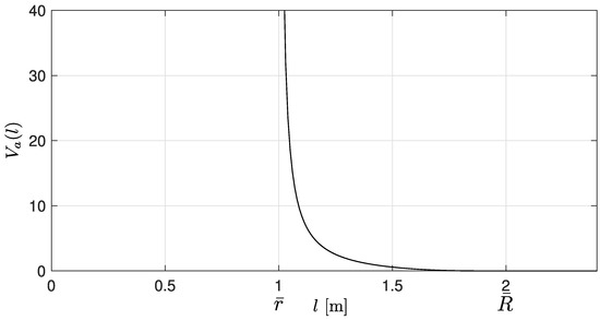
Figure 1.
An example of APF (indexes omitted for simplicity).
Equation (3) fulfills conditions:
As shown in reference [26] it guarantees collision avoidance.
4. Control Algorithm
The goal of the formation control is to mimic motion of the virtual leader maintaining desired displacements between robots and avoiding collisions. It is equivalent to bringing the following quantities to zero:
where and are components of the spatial displacements between robots and i (Figure 2).
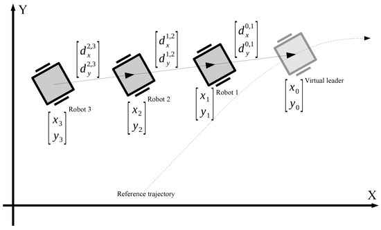
Figure 2.
Leader–follower motion task executed by the formation of three robots.
Assumption 1.
.
This means that the formation is designed in such a way that, when the robots are moving with zero errors, none of them is in the collision avoidance region of other robots.
Assumption 2.
If robot i gets into the collision avoidance region of any other mobile platform j, its desired trajectory is temporarily frozen. If the robot leaves the avoidance area its desired coordinates are immediately updated. As long as the mobile platform remains in the avoidance region, its desired coordinates are periodically updated at certain discrete instants of time. The time period of this update process is relatively large in comparison to the main control loop sample time.
A detailed explanation of this assumption is given in reference [20].
Position and orientation errors expressed with respect to the local coordinate frame fixed to the robot is given by equation:
Accordingly to given model of the robot in Equation (1) the non-holonomic constraint is given by formula:
Using Equations (6) and (7) the error dynamics between robots (the leader) and (the follower) can be expressed as follows:
Position correction variables are introduced that consist of position error and collision avoidance components of control, computed using spatial derivatives of the APFs:
is function of coordinate variables and according to Equations (2) and (3).
To take into account collision avoidance, the error components in the original algorithm from [21] will be replaced by these position correction variables.
Assumption 3.
There are no obstacles other than robots (enumerated …) in the taskspace.
The position correction variables can be expressed in local coordinate frame fixed in the geometric center of the mobile platform:
As shown in reference [24] gradient of the APF can be transformed to be expressed with respect to the local coordinate frame fixed to the i-th mobile robot:
Equation (10) can be rewritten using (9) and (11) as follows:
where each spatial derivative of the APF is transformed from the global to the local coordinate frame fixed to the robot. Correction variables expressed with respect to the local coordinate frame can be written in the following form:
Trajectory tracking algorithm given in [21] extended with collision avoidance based on APF for N mobile platforms is given by equations:
where , , are constant parameters fulfilling conditions , , and function is as follows:
Regardless of the definition of (15) function for replaced by zero in the controller of the i-th robot, it is proposed to keep second term in Equation (14) as in order to avoid possible deadlock.
Assumption 4.
If the value of the linear velocity control is less then considered threshold , i.e., (—positive constant design parameter), it is replaced by a scalar function , where
Above equations can be transformed using (14) and taking into account Assumption 2 (in the collision avoidance region, linear velocity and angular velocities in the i-th robot’s controller are replaced by zero) error dynamics can be rewritten as follows:
The paper [20] presents the same robot control algorithm applied to a formation with a different topology. The stability proof presented there remains valid with the proviso that the error components are defined as in this paper. This indirectly affects , , that are used to compose a Lyapunov-like function. In the stability analysis, the error dynamics (18) was used to derive the system stability condition.
The rule described in Assumption 4 pushes robot out of a state where the stability condition obtained in reference [20] would not be satisfied. This situation occurs when, during collision avoidance, which results from the specific combination of and the sum of the partial derivatives of the APF with respect to the variable , according to the first Equation in (13). The state in which this situation occurs is non-attracting.
5. Experimental Verification
A laboratory setup was prepared for experimental verification of formation control algorithm described in Section 4. The experimental setup description is depicted in Section 5.1. The results obtained from the experiments are presented and later discussed in Section 5.2.
5.1. Experimental Setup
The laboratory experimental setup consists of OptiTrack vision system, MTracker mobile robots and additional PC computer. General scheme of the whole system setup is presented in Figure 3.
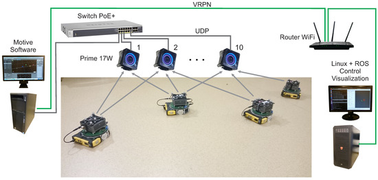
Figure 3.
Experimental setup general scheme.
The OptiTrack vision system includes 10 PRIME 17W cameras, a gigabit PoE network switch for their power supply and communication, and a PC computer with Motive software also connected to this switch. Motive software captures and processes data from cameras. Vision system is responsible for localization of the MTracker mobile robots with use of passive markers placed on the robots that form different so-called rigid bodies (see Figure 4). Based on these markers, the Motive software measures the pose of the robots and distributes these measurements’ results over the local network. During the experiments, the VRPN (Virtual Reality Peripheral Network) protocol has been used to broadcast the measurement information from the vision system. The discussed hardware configuration of the OptiTrack system allows for measurements to be made with a frequency theoretically up to 360 Hz. However, the experiments were carried out at much lower frequencies as will be mentioned later. The arrangement of the cameras allows the robots localization in the available laboratory area of approximately m.
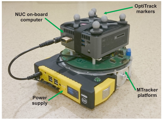
Figure 4.
MTracker mobile robot with equipment.
MTracker robot (see Figure 4) is a small differentially-driven mobile platform with two wheels. It was developed in the Institute of Automatic Control and Robotics at Poznan University of Technology. The mobile platform has a unicycle kinematics which corresponds to the model in Equation (1). The wheels’ base is mm and wheels’ radius is mm. The system is based on DSP (TMS320F28335) low level controller responsible for controlling the motors directly connected with the wheels. This robot platform can be efficiently adopted for realization of experiments with multi-robot systems [27]. For high level control the on-board Intel NUC Mini PC computer has been utilized. Low level controller is connected to NUC computer via USB serial link based on FTDI chip with baud rate 921,600 bps. On-board computer works under Linux Ubuntu 20.04 with ROS Noetic distribution. Each MTracker robot uses the high-level software package with the implementation of the control algorithm. The only difference between the software package versions on each robot is the configuration setup which, for example, defines the number of the robot in the multiple robot formation during the experiments. This gives the ability to easily add more robots to the experimental setup.
In the implemented control system software, each robot has a separate collision avoidance module and a separate controller which makes each robot an independent autonomous unit. This implies that each robot must receive information about the position of all other robots from the vision system responsible for localization. The first robot uses the virtual leader trajectory generator subsystem which was earlier discussed and marked as . Each subsequent robot receives desired velocities of the platform from the preceding robot. A detailed block diagram of the control system architecture for three robots is shown in the Figure 5 and can be easily extended to include other robots in the experimental setup.
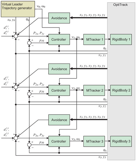
Figure 5.
Functional block scheme of the control system.
The additional desktop PC computer presented in Figure 3 described as Control Visualization also works under Linux Ubuntu with ROS. It works as a master computer running roscore nodes and publishing localization data from VRPN into the ROS network system. It is also used for remote launching of the experimental setup, supervision of the system, visualization and recording of the measurement data and control signals. Data exchange between the master computer and the multiple robots is carried out via a local wireless network using ROS topics and standard messages.
During the experiments robots localization measurements have been done with the frequency of 100 Hz, but the software loop rate in each robot was changed during the experiments. This involved conducting research related to performance of the control algorithm and the robustness of the system for lower frequencies of the control loop.
5.2. Experimental Results
Obtained results of the experiments are presented for the sampling frequency of the control loop at 10 Hz. The experimental verification was carried out with the use of four MTracker robots described in Section 5.1. The experiments were conducted for different robots initial conditions for two different reference trajectories, where the first scenario is marked as EX1 and the second as EX2. Both ware realized with the parameters of the controllers as , and . In the EX1 the trajectory was defined with use of 6th order polynomial continuous function. In the EX2, a circular reference trajectory was given. The spatial offset between successive robots tracking the leader was taken as m and m.
The radius of the area occupied by the robot body was m. At this distance potential function raise to infinity. For greater distances, it falls, reaching zero for m.
For safety reason the maximum angular velocity of the wheels was set to 16 rad/s. In the plots presenting variables evolution colors were used to distinguish different robots: red—, green—, blue— and magenta—. Black color in the last plot of the charts sequence denotes the distances between all robot pairs. Dashed green line shows the collision avoidance area and dashed red line corresponds to radius .
5.2.1. Experiment EX1
Polynomial trajectory in EX1 was generated based on the equations
with (time scaling coefficient) and , , , , , , . The coefficients have been chosen to ensure the feasibility of experiments involving trajectory tracking in available laboratory space. The obtained results for EX1 are presented in Figure 6.
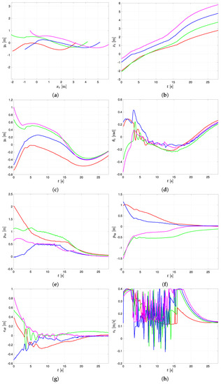
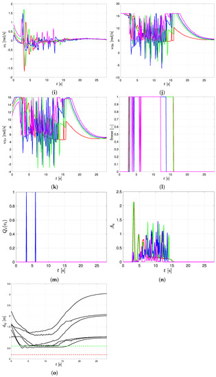
Figure 6.
Experiment EX1—robots execute polynomial trajectory. (a) Locations of the robots on xy-plane; (b–d) Time plots of x, y coordinates and robot orientations respectively; (e–g) Position and orientation errors respectively; (h,i) Linear and angular velocity controls; (j,k) Angular velocities of the wheels; (l) ‘freeze’ signals; (m) activation of the procedure described in Assumption 4 (n) Collision avoidance component of the control Equation (21) (o) Distances between robots.
In the first graph, in Figure 6a, the xy-plot of the robots motion path is shown. In the next ones, time plots of selected signals are presented. The time duration of the experiment was around 27 s and it was related with the speed of the robots and the available laboratory area. Figure 6b,c show x and y position coordinates while Figure 6d orientation of the robots. In Figure 6e–g, the position and orientation errors are presented, respectively. Taking into account these plots one can see that all robots properly follow a trajectory within an assigned formation structure and position errors convergence close to zero.
In Figure 6h,i linear and angular velocity of the calculated control signals is plotted whereas in Figure 6j,k the angular velocities of the robot wheels are depicted. One can see that during the experiment velocities of the wheels reached fixed limit. Figure 6l shows ‘freeze’ signals which equals 1, indicate that the reference signals was frozen to avoid collision between robots.
During the transient state of the motion collision avoidance mechanism was activated what is presented by the ‘freeze’ signals plot. Freezing the reference signals can be easily observed as resulting in some chattering of the linear velocity and especially in wheels velocity signals. Collision avoidance behavior prevented the robots from coming closer than m to each other (see Figure 6o). The threshold distance of ‘freeze’ signal activation was equal to the radius of the collision avoidance area m (dashed green line). As robots get closer to each other, the distance collision avoidance blocks cause repulsion between robots. As all robots maintained a distance greater than m (dashed red line) between each other, no collision occurred. Figure 6m shows signals:
that represent activation of the procedure described in Assumption 4. The value of the threshold was set to m/s. This procedure was activated twice during the experiment, for a short period of time. It temporarily disrupts the robot’s motion, but prevents it from getting stuck.
The collision avoidance component of the control is shown in Figure 6n. It is a norm of the sum of all collision avoidance vectors acting on the i-th robot:
The signals are non-zero only if the robots are close enough to each other (at a distance less than ).
Figure 6o presents the situation when the robots reach their trajectories, the relative distances between them are close to desired value equal to m. The green dashed line denotes the distance and red dashed line is the distance at which the collision would occur. As can be seen, the distances between all the robots remain safe during the experiment, reaching values only slightly smaller than .
5.2.2. Experiment EX2
In the EX2 desired circular trajectory was generated according to the equations
with m and rad/s. The results of the experiment are presented in the Figure 7. The individual graphs are arranged similarly as in the EX1. Because of closed circle shape of the trajectory the duration of EX2 is longer then in EX1.
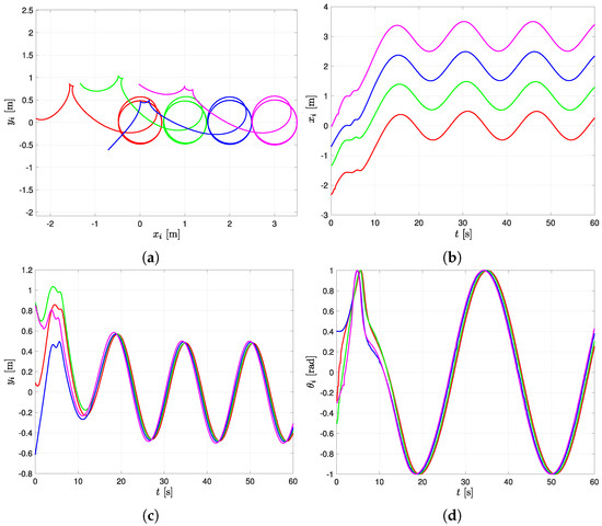
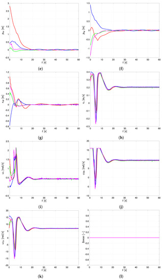
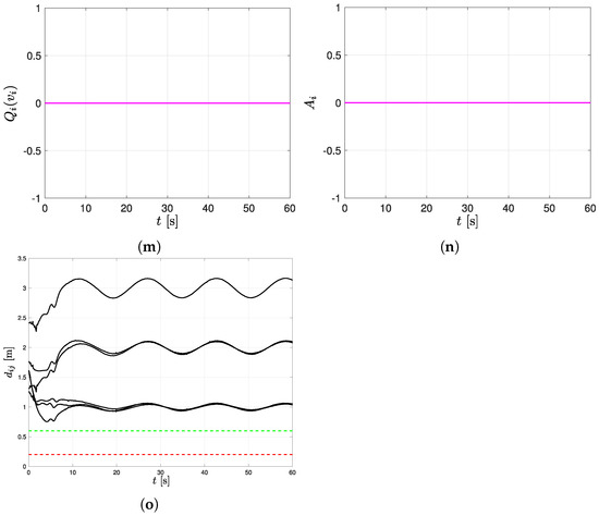
Figure 7.
Experiment EX2—robots execute circular trajectory. (a) Locations of the robots on xy-plane. (b–d) Time plots of x, y coordinates and robot orientations respectively. (e–g) Position and orientation errors respectively. (h,i) Linear and angular velocity controls. (j,k) Angular velocities of the wheels. (l) ‘freeze’ signals. (m) activation of the procedure described in Assumption 4 (n) Collision avoidance component of the control Equation (21) (o) Distances between robots.
Figure 7a shows xy-plot of the robots movement. Figure 7b,c present x and y position coordinates and Figure 7d orientation of the robots. In Figure 7e–g position and orientation errors are depicted, respectively. Consistently, in Figure 7h,i linear and angular velocity control signals are plotted. Figure 7j,k show angular velocities of the wheels. One can see that after a period of about 10 s the transient state of each robot movement ends and the robots’ formation starts to follow the trajectory precisely, what means that errors are close to zero.
For such robots, the initial conditions collision avoidance behavior has not been activated. This can be observed in Figure 7l–n where all signals are equal to zero all the time. Although the initial positions of the robots were quite far from desired, they did not approach each other at a distances at which the collision avoidance block would be activate. Consequently, the velocities are smoother compared to the EX1, although velocities of the wheels also reach the limit during the transient state. The setting time is slightly shorter.
Figure 7o also confirms that no collision occurred during the EX2. The relative distances between robots are greater than m (green dashed line). In the final stage, the assumed offsets are preserved as well.
6. Conclusions
According to our knowledge, this is the first time where the experimental results are considered for the control approach discussed in this paper. We focus on analysis and implementation of the control algorithm for differentially-driven mobile robots based on the leader–follower idea. Conducted experiments show applicable performance of this approach in the distributed system. The robots correctly achieve and move in the assumed formation following the reference trajectory. Implemented controller with collision avoidance strategy which is based on artificial potential functions effectively prevent collisions. The experiments were carried out with the use of four robots, but the prepared system setup allows us to increase the number of robots without the need to modify the developed control architecture. The authors plan to extend this approach to tracking the leader using the mobile robot’s on-board sensor system instead of the OptiTrack vision system.
Author Contributions
Conceptualization, W.K.; methodology, M.K. and B.K.; software, M.K., W.K. and B.K.; validation, M.K., W.K. and B.K.; formal analysis, W.K. and B.K.; investigation, M.K., W.K. and B.K.; resources, M.K. and B.K.; data curation, M.K. and W.K.; writing—original draft preparation, M.K. and W.K.; writing—review and editing, M.K., W.K. and B.K.; visualization, M.K. and W.K. All authors have read and agreed to the published version of the manuscript.
Funding
This work is supported by statutory grant 0211/SBAD/0122.
Institutional Review Board Statement
Not applicable.
Informed Consent Statement
Not applicable.
Data Availability Statement
Not applicable.
Conflicts of Interest
The authors declare no conflict of interest.
References
- Huntsberger, T.L.; Trebi-Ollennu, A.; Aghazarian, H.; Schenker, P.S.; Pirjanian, P.; Nayar, H.D. Distributed Control of Multi-Robot Systems Engaged in Tightly Coupled Tasks. Auton. Robot. 2004, 17, 79–92. [Google Scholar] [CrossRef]
- Valbuena Reyes, L.A.; Tanner, H.G. Flocking, Formation Control, and Path Following for a Group of Mobile Robots. IEEE Trans. Control Syst. Technol. 2015, 23, 1268–1282. [Google Scholar] [CrossRef]
- Lytridis, C.; Kaburlasos, V.G.; Pachidis, T.; Manios, M.; Vrochidou, E.; Kalampokas, T.; Chatzistamatis, S. An Overview of Cooperative Robotics in Agriculture. Agronomy 2021, 11, 1818. [Google Scholar] [CrossRef]
- Rashid, A.T.; Abdulrazaaq, B. A Survey of Multi-mobile Robot Formation Control. Int. J. Comput. Appl. 2019, 181, 12–16. [Google Scholar] [CrossRef]
- Tsiu, L.; Markus, E.D. A Survey of Formation Control for Multiple Mobile Robotic Systems. Int. J. Mech. Eng. Robot. Res. 2020, 9, 1515–1520. [Google Scholar] [CrossRef]
- Kamel, M.A.; Yu, X.; Zhang, Y. Fault-Tolerant Cooperative Control Design of Multiple Wheeled Mobile Robots. IEEE Trans. Control Syst. Technol. 2018, 26, 756–764. [Google Scholar] [CrossRef]
- Wu, W.; Zhang, F. Robust Cooperative Exploration with a Switching Strategy. IEEE Trans. Robot. 2012, 28, 828–839. [Google Scholar] [CrossRef]
- Wei, H.; Lv, Q.; Duo, N.; Wang, G.; Liang, B. Consensus Algorithms Based Multi-Robot Formation Control under Noise and Time Delay Conditions. Appl. Sci. 2019, 9, 1004. [Google Scholar] [CrossRef]
- Jin, J.; Kim, Y.; Wee, S.; Gans, N. Consensus based attractive vector approach for formation control of nonholonomic mobile robots. In Proceedings of the IEEE International Conference on Advanced Intelligent Mechatronics (AIM), Busan, Korea, 7–11 July 2015. [Google Scholar] [CrossRef]
- Du, H.; Wen, G.; Cheng, Y.; He, Y.; Jia, R. Distributed Finite-Time Cooperative Control of Multiple High-Order Nonholonomic Mobile Robots. IEEE Trans. Neural Netw. Learn. Syst. 2017, 28, 2998–3006. [Google Scholar] [CrossRef]
- Gutiérrez, H.; Morales, A.; Nijmeijer, H. Synchronization Control for a Swarm of Unicycle Robots: Analysis of Different Controller Topologies. Asian J. Control 2017, 19, 1822–1833. [Google Scholar] [CrossRef]
- Yang, T.T.; Liu, Z.Y.; Chen, H.; Pei, R. Formation Control and Obstacle Avoidance for Multiple Mobile Robots. Acta Automat. Sin. 2008, 34, 588–593. [Google Scholar] [CrossRef]
- Zhang, Q.; Lapierre, L.; Xiang, X. Distributed control of coordinated path tracking for networked nonholonomic mobile vehicles. IEEE Trans. Ind. Inform. 2013, 9, 472–484. [Google Scholar] [CrossRef]
- Nguyen, D.B.; Do, K.D. Formation Control of Mobile Robots. Int. J. Comput. Commun. Control 2006, 1, 41–59. [Google Scholar] [CrossRef][Green Version]
- Kowalczyk, W. Formation Control and Distributed Goal Assignment for Multi-Agent Non-Holonomic Systems. Appl. Sci. 2019, 9, 1311. [Google Scholar] [CrossRef]
- Panagou, D.; Kumar, V. Cooperative Visibility Maintenance for Leader–Follower Formations in Obstacle Environments. IEEE Trans. Robot. 2014, 30, 831–844. [Google Scholar] [CrossRef]
- Miao, Z.; Zhong, H.; Lin, J.; Wang, Y.; Chen, Y.; Fierro, R. Vision-Based Formation Control of Mobile Robots with FOV Constraints and Unknown Feature Depth. IEEE Trans. Control Syst. Technol. 2021, 29, 2231–2238. [Google Scholar] [CrossRef]
- Hirata-Acosta, J.; Pliego-Jiménez, J.; Cruz-Hernádez, C.; Martínez-Clark, R. Leader–follower Formation Control of Wheeled Mobile Robots without Attitude Measurements. Appl. Sci. 2021, 11, 5639. [Google Scholar] [CrossRef]
- Wang, B.; Ashrafiuon, H.; Nersesov, S. Leader–follower formation stabilization and tracking control for heterogeneous planar underactuated vehicle networks. Syst. Control Lett. 2021, 156, 105008. [Google Scholar] [CrossRef]
- Kozlowski, K.; Kowalczyk, W. Control of Two-wheeled Mobile Robots Moving in Formation. IFAC-PapersOnLine 2020, 53, 9608–9613. [Google Scholar] [CrossRef]
- Canudas de Wit, C.; Khennouf, H.; Samson, C.; Sordalen, O.J. Nonlinear Control Design for Mobile Robots. Recent Trends Mob. Rob. 1994, 121–156. [Google Scholar] [CrossRef]
- Loria, A.; Dasdemir, J.; Alvarez Jarquin, N. Leader—Follower Formation and Tracking Control of Mobile Robots Along Straight Paths. IEEE Trans. Control Syst. Technol. 2016, 24, 727–732. [Google Scholar] [CrossRef]
- Khatib, O. Real-time obstacle avoidance for manipulators and mobile robots. Int. J. Rob. Res. 1986, 5, 90–98. [Google Scholar] [CrossRef]
- Kowalczyk, W.; Kozłowski, K. Trajectory tracking and collision avoidance for the formation of two-wheeled mobile robots. Bull. Pol. Acad. Sci. Tech. Sci. 2019, 67, 915–924. [Google Scholar] [CrossRef]
- Kowalczyk, W.; Kozłowski, K.; Tar, J.K. Trajectory tracking for multiple unicycles in the environment with obstacles. In Proceedings of the 19th International Workshop on Robotics in Alpe-Adria-Danube Region (RAAD 2010), Budapest, Hungary, 23–27 June 2010; pp. 451–456. [Google Scholar]
- Mastellone, S.; Stipanovic, D.M.; Graunke, C.R.; Intlekofer, K.A.; Spong, M.W. Formation control and collision avoidance for multi-agent non-holonomic systems: Theory and experiments. Int. J. Rob. Res. 2008, 27, 107–126. [Google Scholar] [CrossRef]
- Kozlowski, K.; Kowalczyk, W.; Krysiak, B.; Kielczewski, M.; Jedwabny, T. Modular Architecture of the Multi-robot System for Teleoperation and Formation Control Purposes. In Proceedings of the 9th International Workshop on Robot Motion and Control (RoMoCo), Wasowo Palace, Poland, 3–5 July 2013. [Google Scholar] [CrossRef]
Publisher’s Note: MDPI stays neutral with regard to jurisdictional claims in published maps and institutional affiliations. |
© 2022 by the authors. Licensee MDPI, Basel, Switzerland. This article is an open access article distributed under the terms and conditions of the Creative Commons Attribution (CC BY) license (https://creativecommons.org/licenses/by/4.0/).