
Comparative Assessment of Shear Demand for RC Beam-Column Joints under Earthquake Loading


Abstract
:1. Introduction
2. Fundamentals of RC Beam-Column Joints
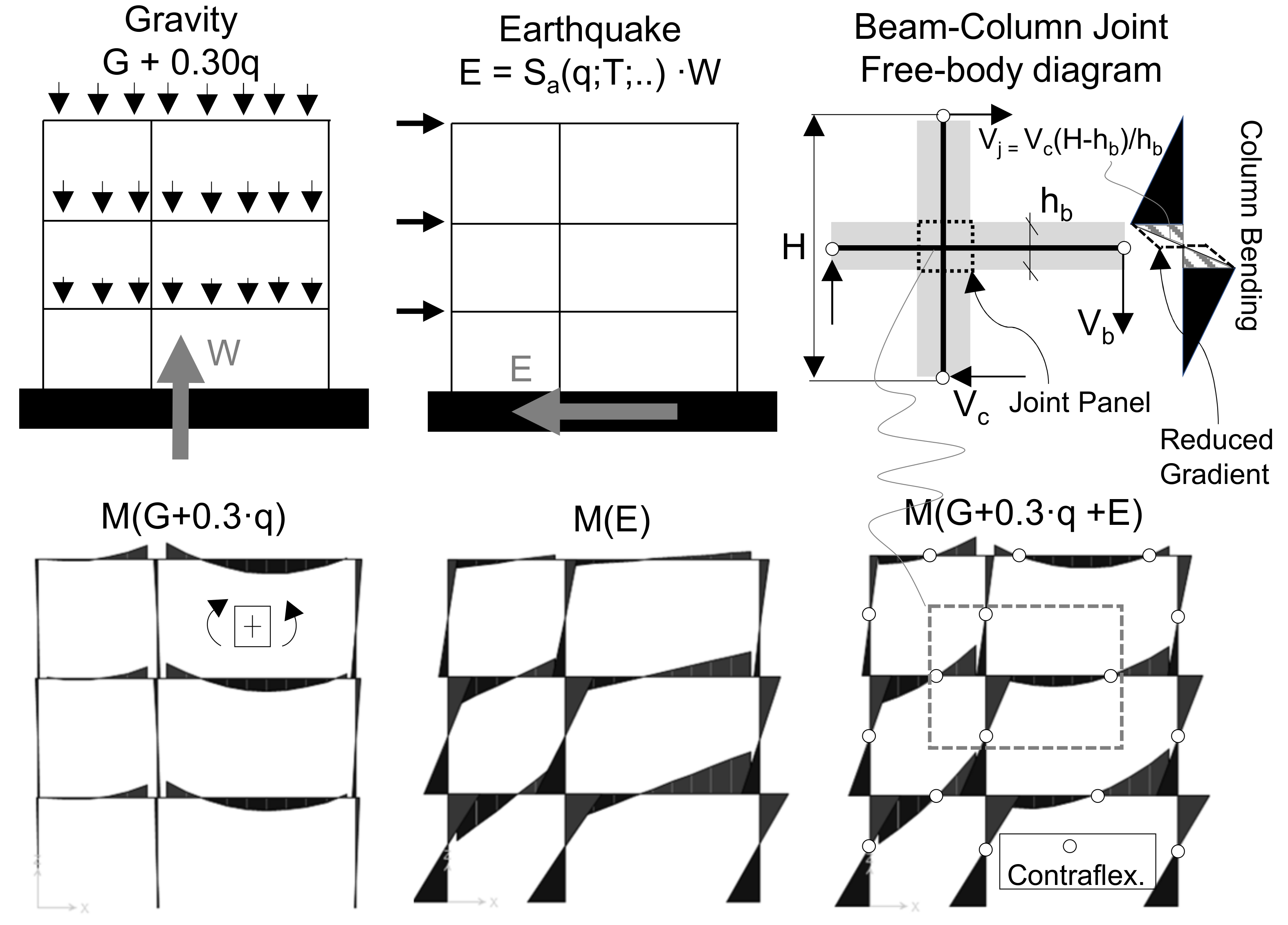
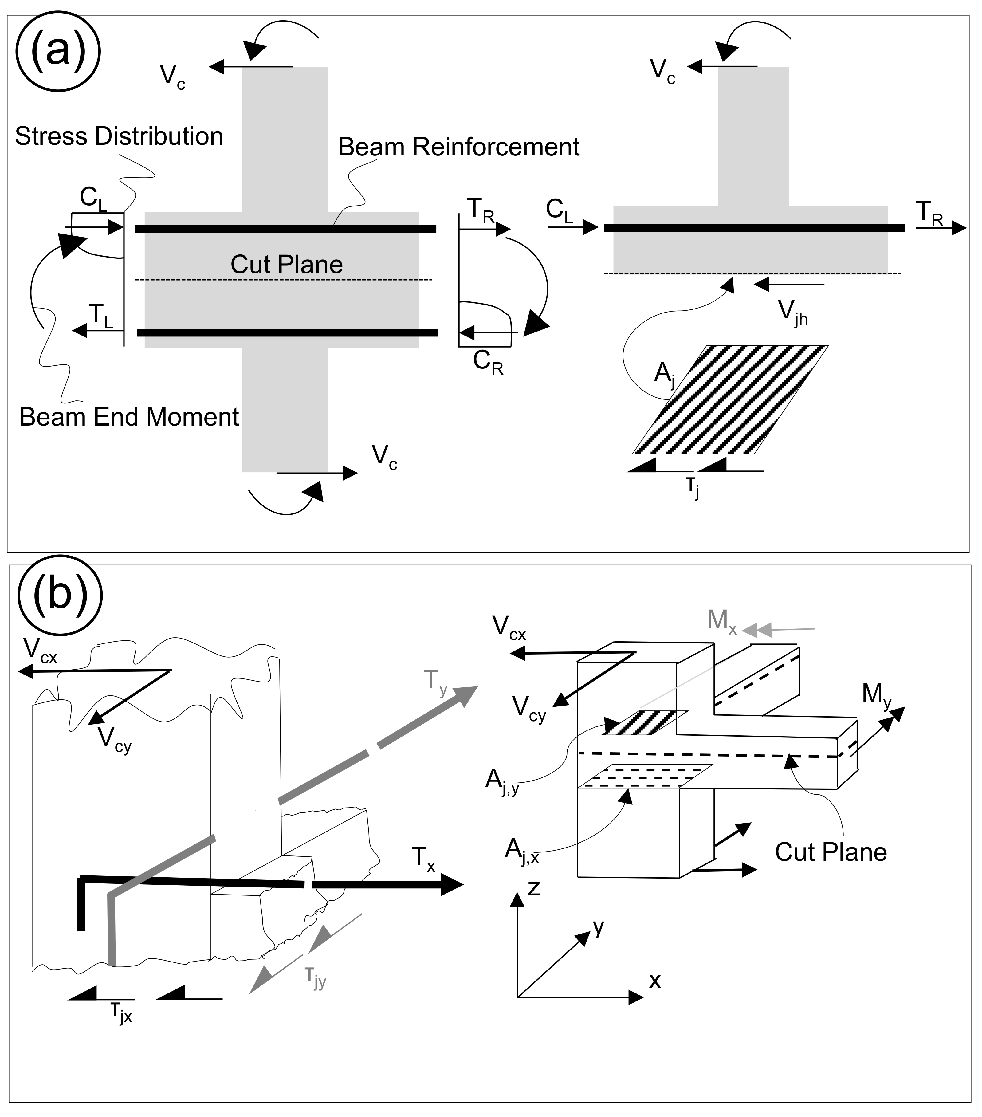
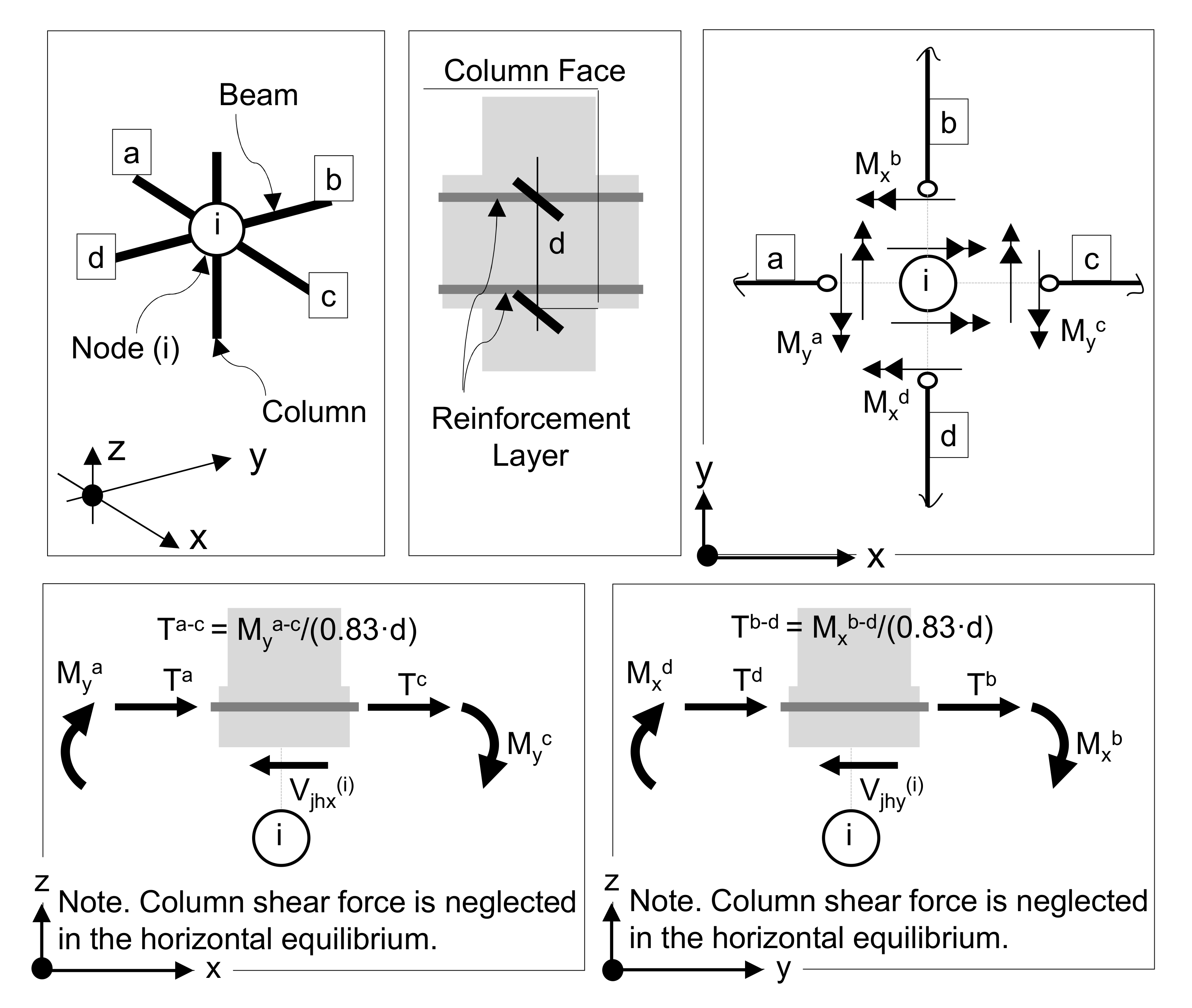
2.1. Joint Shear Demand
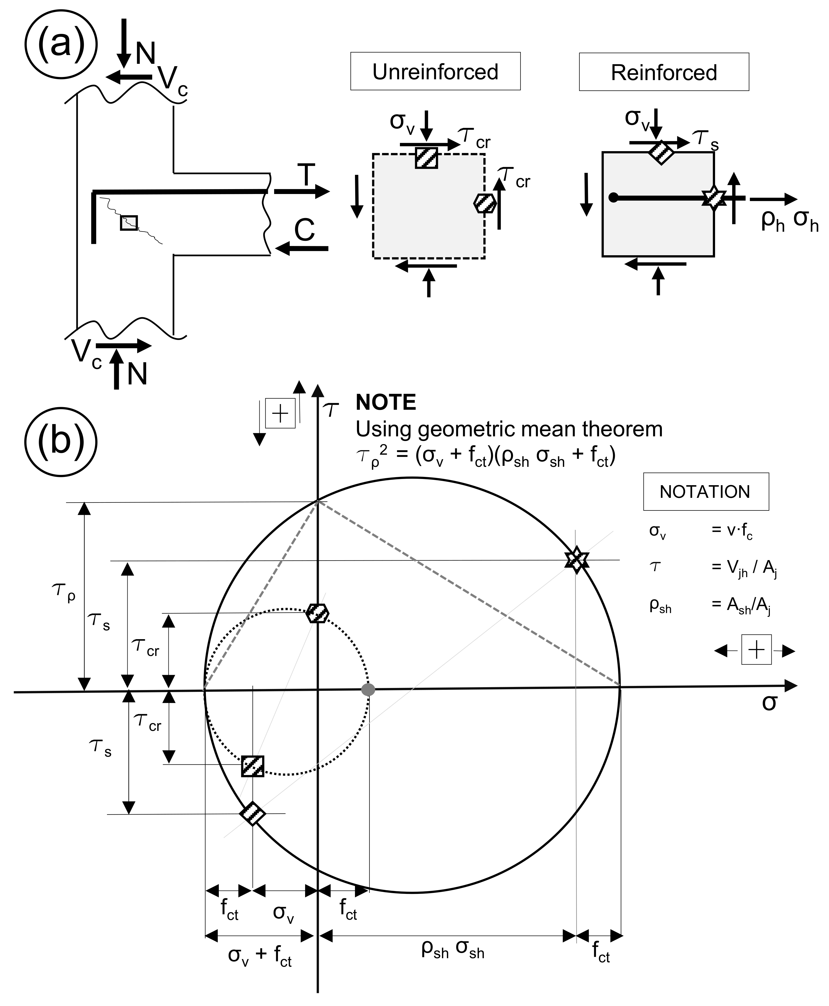
2.2. Joint Shear Strength
2.2.1. Ec8
- is the reinforcement ratio;
- is the normalized axial force.
2.2.2. Nzsee-2017
2.2.3. Asce41-17
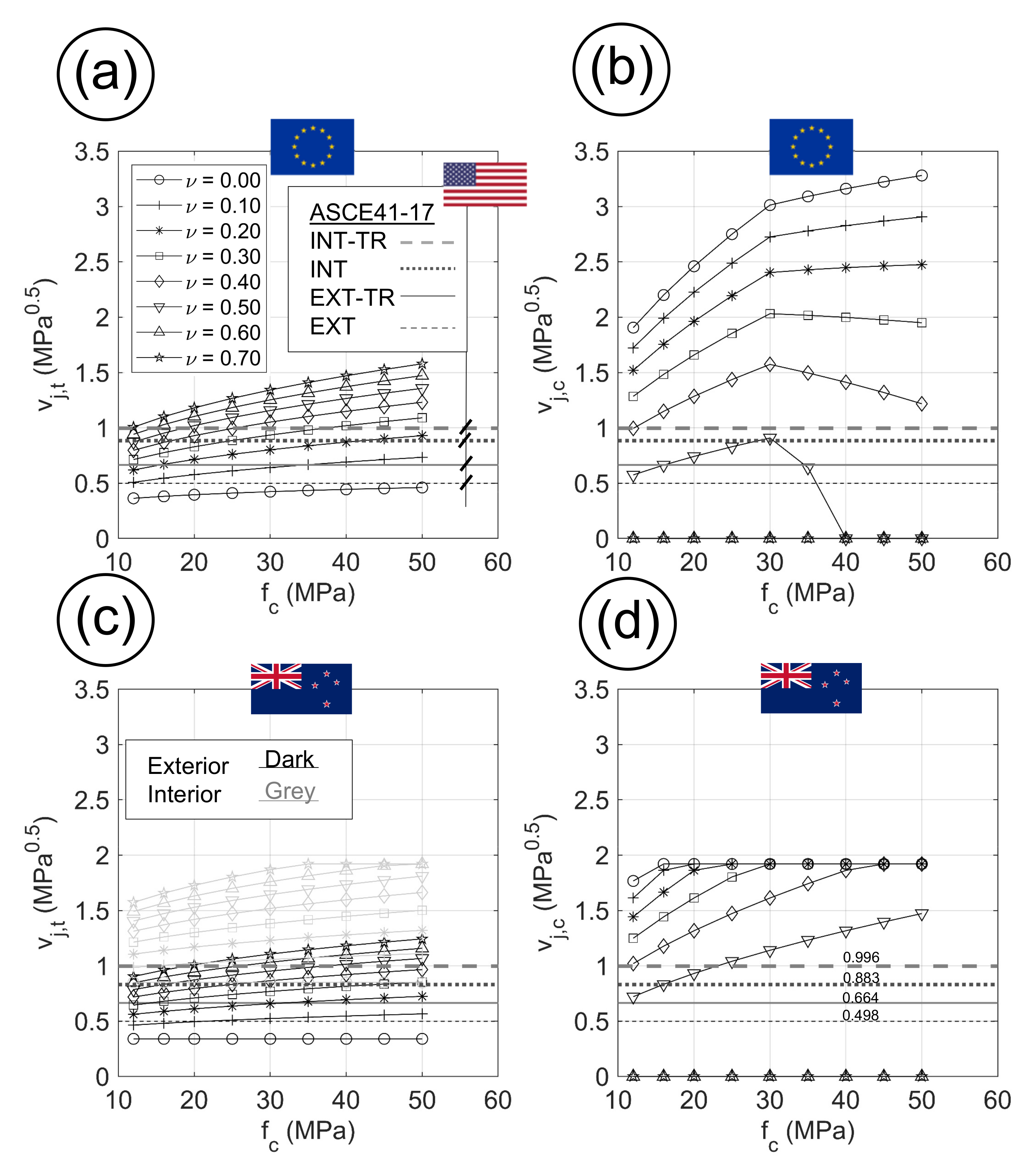
2.2.4. Parametrical Comparison
3. Numerical Study
3.1. Scope
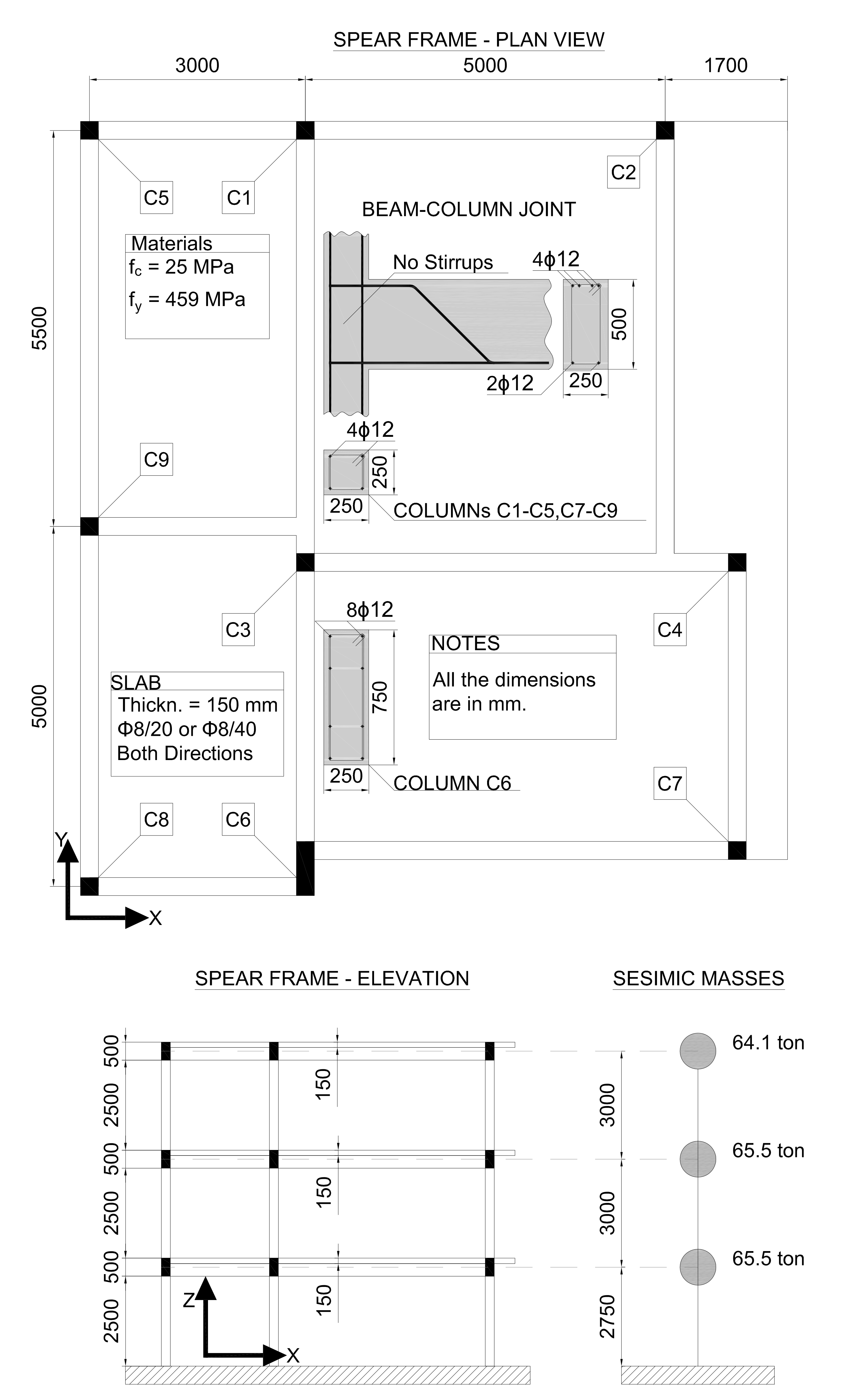
3.2. Details of SPEAR Frame
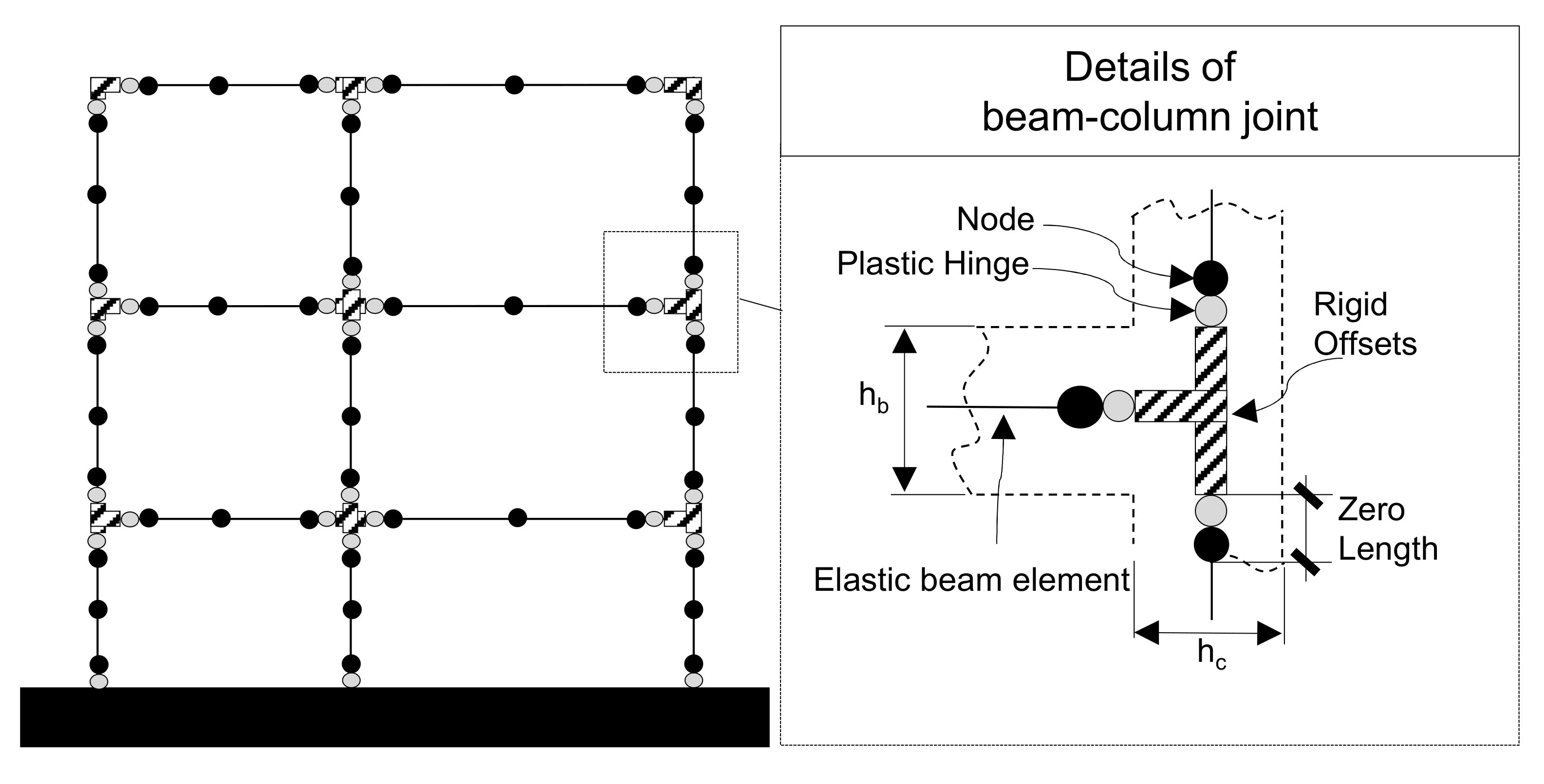
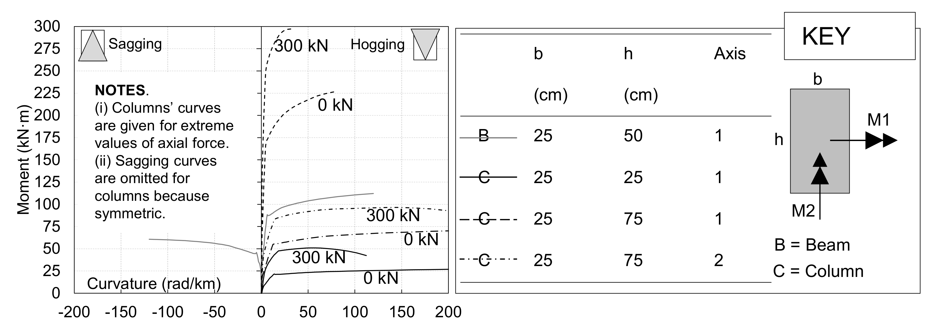
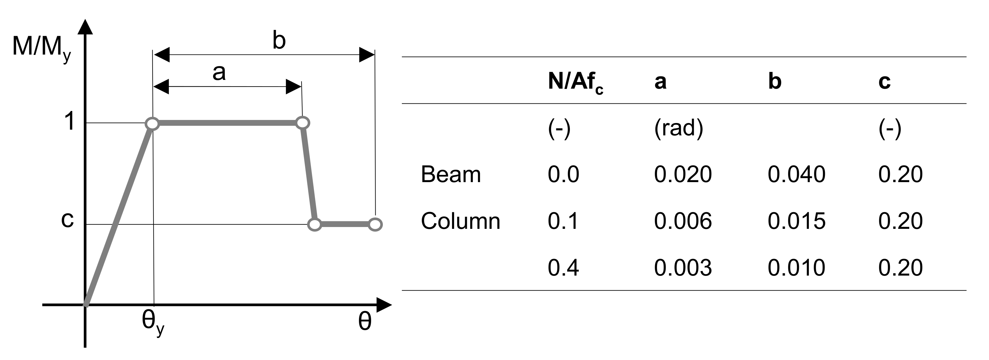
3.3. Structural Modeling and Seismic Demand
3.4. Validation
4. Results and Discussion
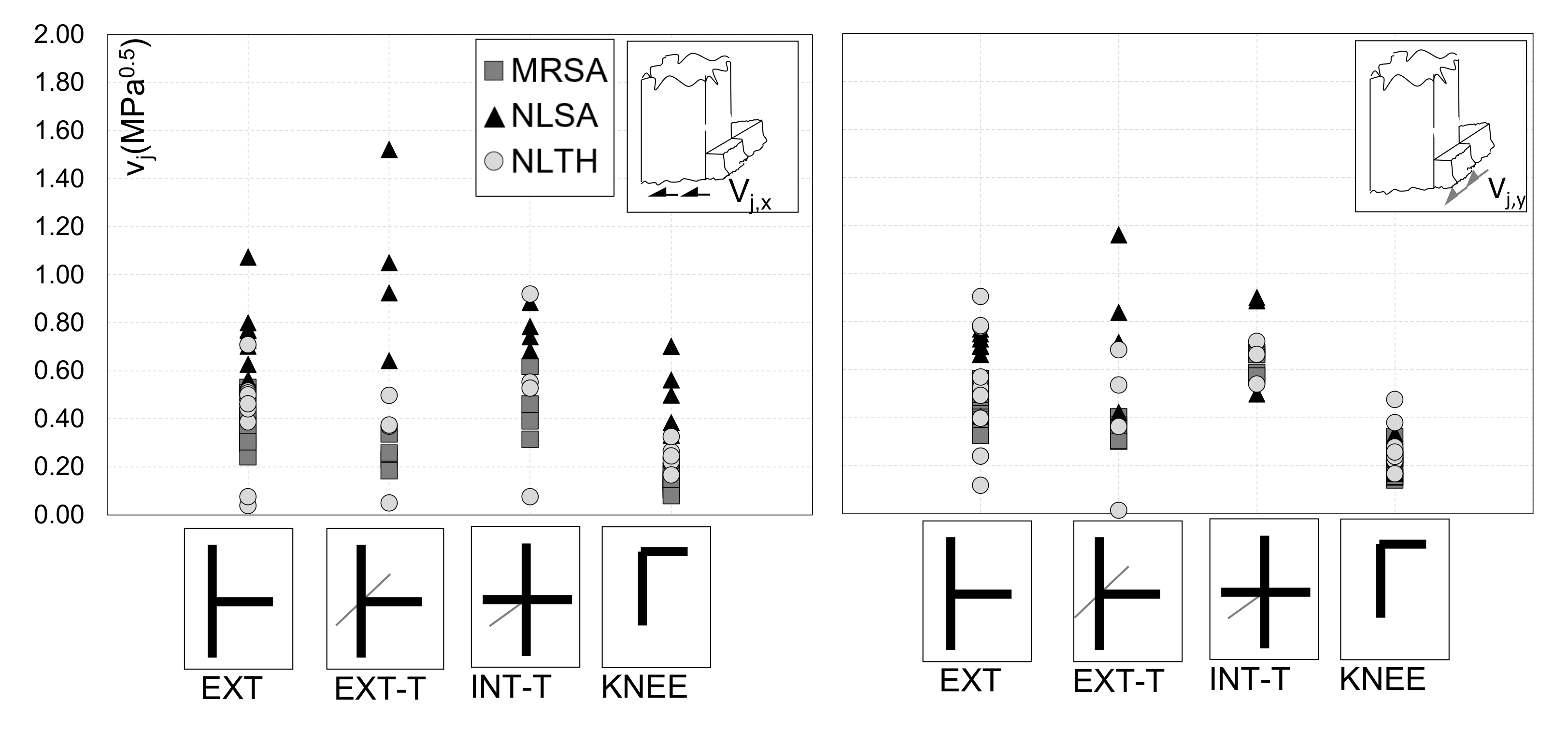
4.1. Shear Demand at a Joint
- (MRSA) Maximum values of shear demand at a joint are evaluated, considering the 30% rule for the bi-directional combination. Modal contributions were summed using the complete-quadratic combination (CQC);
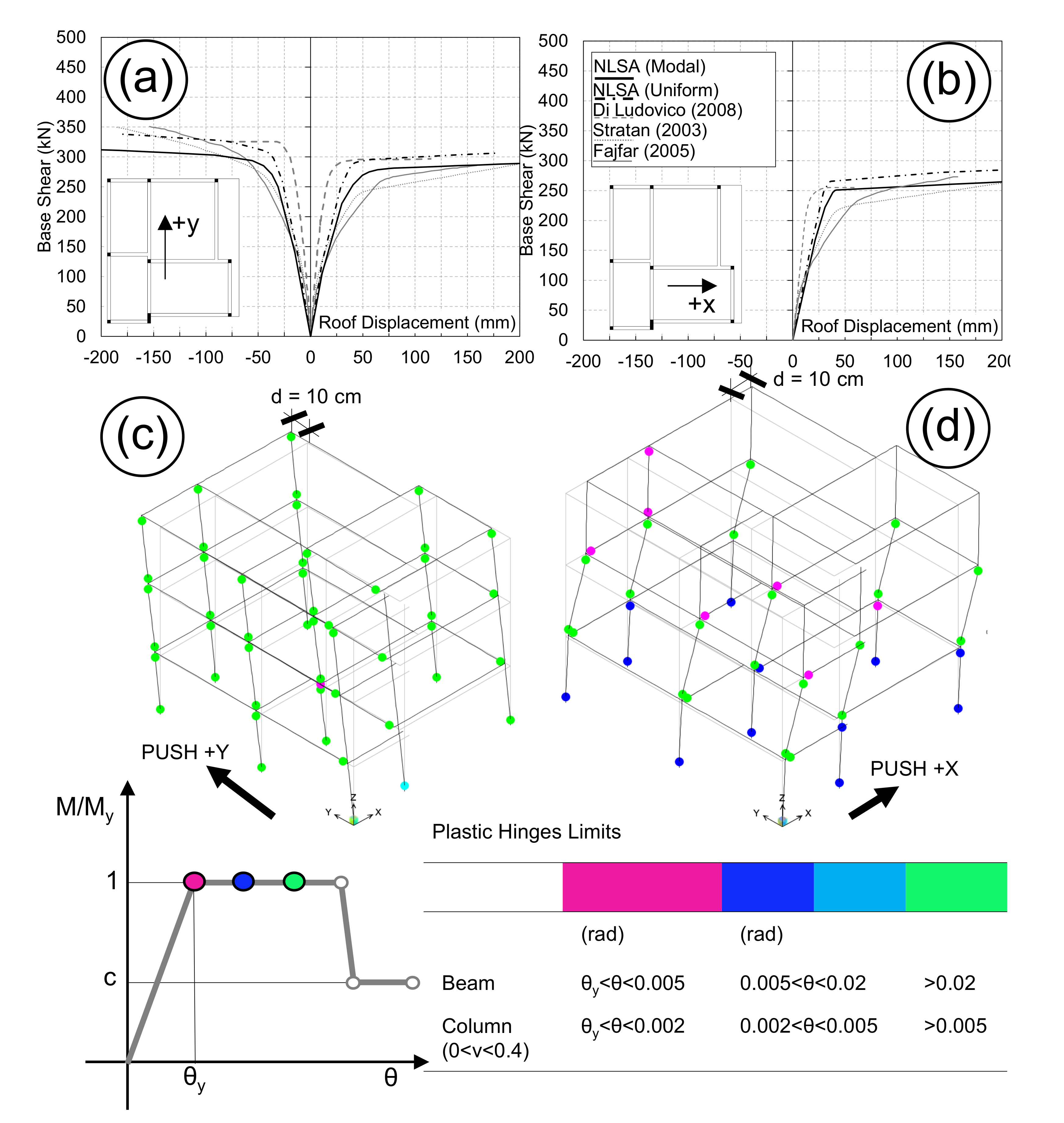
- (NLSA) Pushover curves were calculated using the modal force distribution for the first three modes. Specifically, target displacements were assumed in the x-direction for the mode “1” and in the y-direction for the mode “2”. Mode “3” being torsional, both the ±x and ±y directions of target displacements were considered. Subsequently, idealization of the pushover curve into a bi-linear curve is made. Shear demand at a joint is extracted for each idealized pushover curve, at the target displacement. The final shear demand is then computed, summing the modal contribution using CQC. This procedure is compliant with what was proposed by Chopra [46], named modal-pushover-analysis (MPA);
- (NLTH) Extreme values of shear demand at a joint are extracted from time histories. Acceleration of time histories apply simultaneously in ±x and ±y directions. Envelope of the results coming from different direction signs is made.
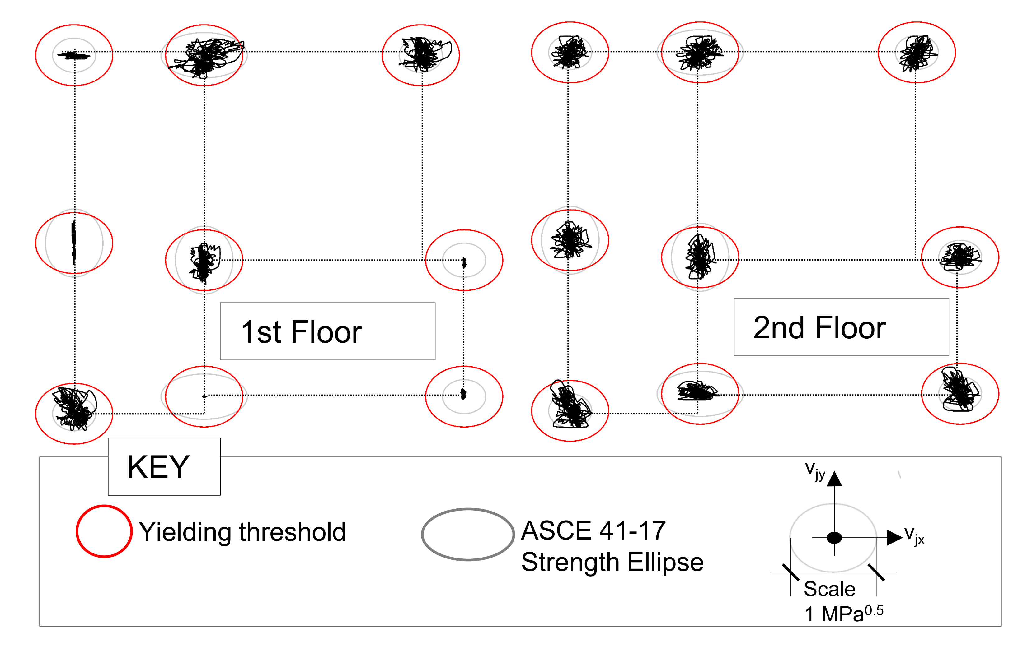
4.2. Bi-Axial Shear Demand Using NLTH
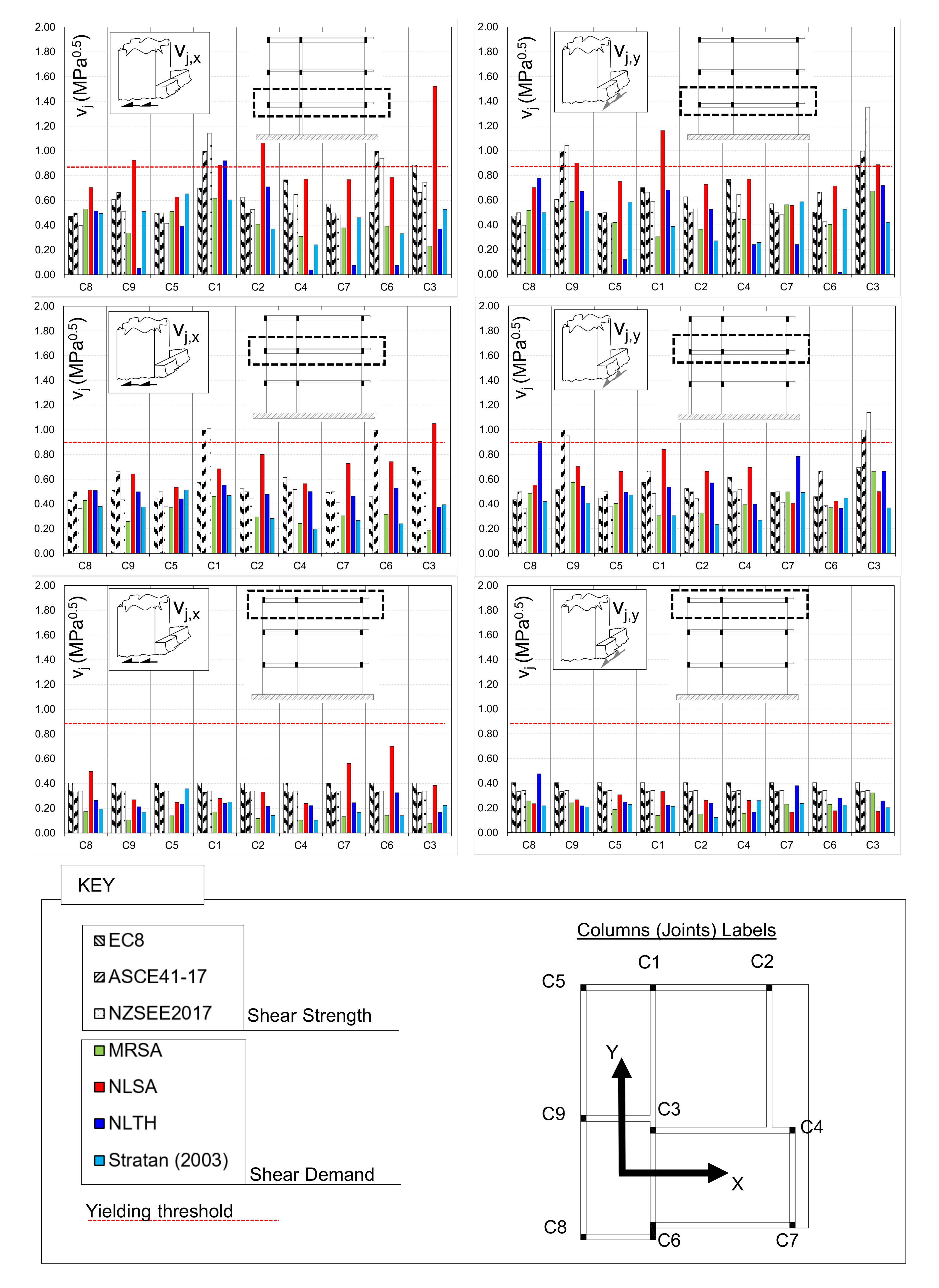
4.3. Evaluated Shear Strength
4.4. Comparison of Shear Demands
5. Conclusions
- 1.
- The shear demand at a beam–column joint being a non-conventional output, a post-process based on nodal moments is needed. Two major hypotheses were made: (i) the internal lever arm at the column face cross section, of the beam, was assumed constant and (ii) the contribution to the horizontal equilibrium of the column’s shear was neglected. The last assumption’s results are conservative;
- 2.
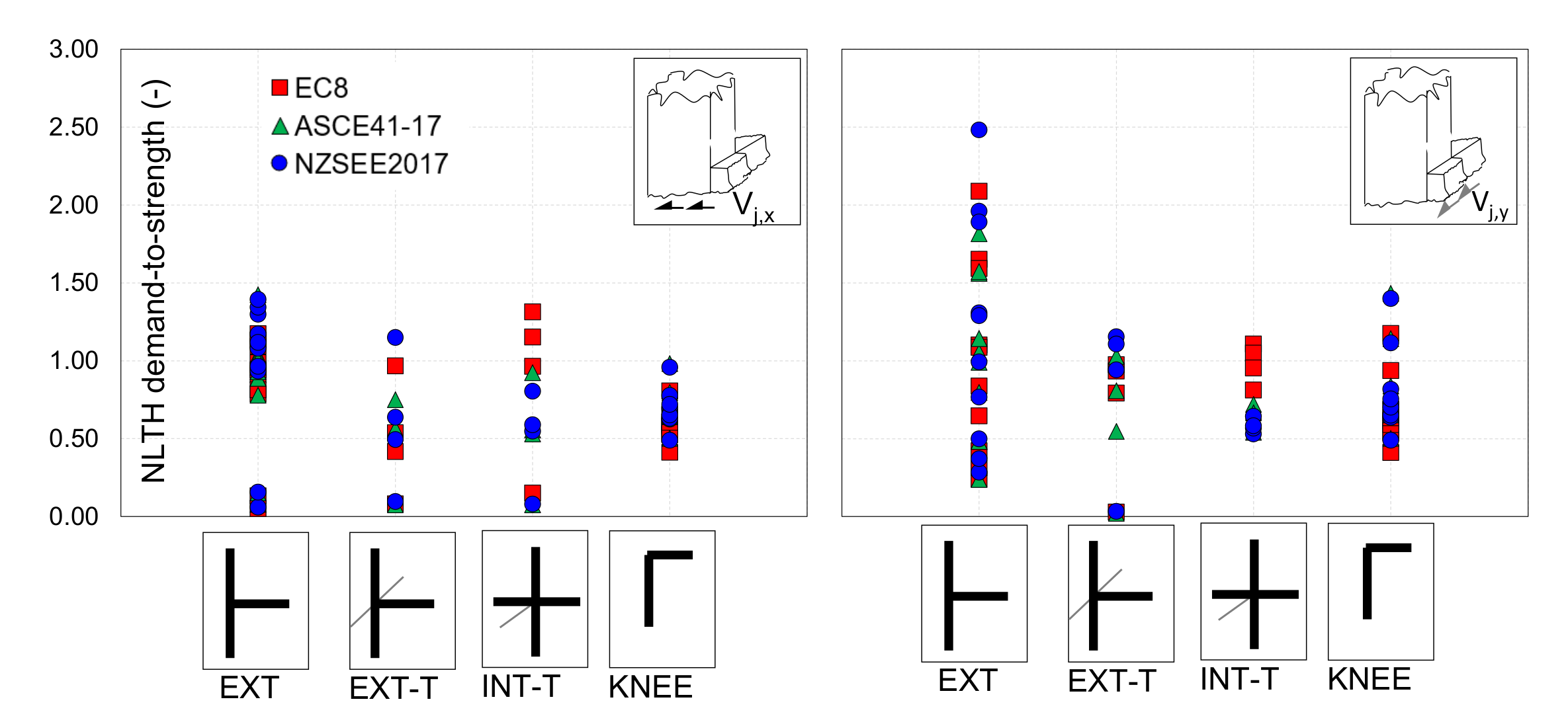
- Shear strength evaluation should be extended to all the beam–column joints in a three-dimensional frame, distinguishing two flexural planes. Significant strength differences might be influenced by (i) the joint type attribute in each flexural plane and (ii) the use of different building codes;
- 3.
- The larger safety margin was recognized for corner joints by assigning to them the exterior joint type in both the flexural planes. Larger strength should be expected as a result of the confinement offered by the beams in both directions. Besides, elliptical strength interaction domain results were conservative when compared with NLTH shear demand orbits;
- 4.
- Among the reviewed building codes, EC8 produced larger strength predictions than ASCE41-17 and NZSEE2017. The latter produced the lowest ones. Discussion about the strength accuracy was not intended because the compared shear demands represent a condition far from failure;
- 5.
- NLSA was proven to estimate the larger shear demand with respect to MRSA and NLTH. Differences were explained as a consequence of the possible inaccuracy of NLSA, using modal combination, in the evaluation of elements’ forces. Such evidence needs to be investigated further since NLSA is frequently adopted in the assessment of existing RC structures as a compromise between MRSA and NLTH.
Author Contributions
Funding
Data Availability Statement
Acknowledgments
Conflicts of Interest
Abbreviations
| CQC | Complete Quadratic Combination |
| dofs | degrees-of-freedom |
| MPA | Modal-pushover-Analysis |
| MRSA | Modal Response Spectrum |
| NLSA | Non-Linear Static Analysis |
| NLTH | Non-Linear Time History |
| PGA | Peak Ground Acceleration |
| PsD | Pseudo-dynamic |
| RC | Reinforced Concrete |
References
- Varum, H. Seismic Assessment, Strengthening and Repair of Existing Buildings. Ph.D. Thesis, Universidade de Aveiro, Aveiro, Portugal, 2003. [Google Scholar]
- Kam, W.Y.; Pampanin, S.; Elwood, K. Seismic performance of reinforced concrete buildings in the 22 February Christchurch (Lyttelton) earthquake. Bull. N. Z. Soc. Earthq. Eng. 2011, 44, 239–278. [Google Scholar] [CrossRef] [Green Version]
- Pantazopoulou, S.; Bonacci, J. On earthquake-resistant reinforced concrete frame connections. Can. J. Civ. Eng. 1994, 21, 307–324. [Google Scholar] [CrossRef]
- Parate, K.; Kumar, R. Shear strength criteria for design of RC beam–column joints in building codes. Bull. Earthq. Eng. 2019, 17, 1407–1493. [Google Scholar] [CrossRef]
- Celik, O.C.; Ellingwood, B.R. Modeling beam–column joints in fragility assessment of gravity load designed reinforced concrete frames. J. Earthq. Eng. 2008, 12, 357–381. [Google Scholar] [CrossRef]
- Moehle, J.P. Seismic Deisgn of RC Buildings; McGraw-Hill Education: New York, NY, USA, 2015. [Google Scholar] [CrossRef]
- Negro, P.; Fardis, M.N. Seismic Performance Assessment and Rehabilitation of Existing Buildings (SPEAR) International Workshop Proceedings; Office for Official Publication of the European Communities: Luxembourg, 2005. [Google Scholar]
- Paulay, T.; Priestley, N. Seismic Design for Concrete and Masonry Buildings; Wiley: New York, NY, USA, 1992. [Google Scholar]
- ACI. ACI 318-19 Building Code Requirements for Structural Concrete and Commentary; American Concrete Institute (ACI): Farmington Hills, MI, USA, 2019. [Google Scholar] [CrossRef]
- EN 1998-1:2004; Eurocode 8: Design of Structures for Earthquake Resistance. Part1: General Rules, Seismic Actions and Rules for Buildings. European Committee for Standardization (CEN): Brussels, Belgium, 2004.
- ACI 352R-02; Recommendations for Design of Beam-Column Connections in Monolithic Reinforced Concrete Structures (ACI-ASCE 352-02). American Concrete Institute (ACI): Farmington Hills, MI, USA, 2002.
- CEN/TC250/SC8; prEN1998-1-3:2022; Eurocode 8: Design of Structures for Earthquake Resistance. Part 1-3: Assessment and Retrofitting of Buildings and Bridges. European Committee for Standardization (CEN): Brussels, Belgium, 2004.
- NZSEE. The Seismic Assessement of Existing Building; Technical Report; New Zeland Society of Earthquake Engineering: Wellington, New Zealand, 2017. [Google Scholar]
- ASCE. ASCE/SEI, 41-17 Seismic Evaluation and Retrofit of Existing Buildings; American Society of Civil Engineers: Reston, VA, USA, 2017; p. 623. [Google Scholar]
- Oloukun, F.A. Prediction of concrete tensile strength from compressive strength: Evaluation of existing relations for normal weight. ACI Mater. J. 1991, 88, 302–309. [Google Scholar]
- Hakuto, S.; Park, R.; Tanaka, H. Seismic Load Test on Interior and Exterior Beam-Column Joints with Substandards Reinforcing Details. ACI J. 2000, 97, 11–25. [Google Scholar]
- Kosmopoulos, A.; Fardis, M.N. Estimation of inelastic seismic deformations in asymmetric multistorey RC buildings. Earthq. Eng. Struct. Dyn. 2007, 36, 1209–1234. [Google Scholar] [CrossRef]
- Di Ludovico, M. Seismic Behavior of a Full-Scale RC Structure Retrofitted Using GFRP Laminates. J. Struct. Eng. 2008, 134, 810–821. [Google Scholar] [CrossRef]
- Negro, P.; Mola, E.; Molina, F.J.; Magonette, G.E. Full-scale PsD testing of a torsionally unbalanced three-storey non-seismic RC frame. In Proceedings of the 13th World Conference on Earthquake Engineering, Vancouver, BC, Canada, 1–6 August 2004; p. 968. [Google Scholar]
- Molina, F.J.; Negro, P. Bidirectional pseudodynamic technique for testing a three-storey reinforced concrete building. In Proceedings of the 13th World Conference on Earthquake Engineering, Vancouver, BC, Canada, 1–6 August 2004; p. 75. [Google Scholar]
- Reynouard, J.M.; Ile, N.; Brun, M. Inelastic seismic analysis of the SPEAR test building. Eur. J. Environ. Civ. Eng. 2010, 14, 855–867. [Google Scholar] [CrossRef]
- Bento, R.; Bhatt, C.; Pinho, R. Using nonlinear static procedures for seismic assessment of the 3D irregular SPEAR building. Earthq. Struct. 2010, 1, 177–195. [Google Scholar] [CrossRef]
- Freeman, S.A. Review of the Development of the Capacity Spectrum Method. ISET J. Earthq. Technol. 2004, 41, 113. [Google Scholar]
- Bhatt, C.; Bento, R. Extension of the CSM-FEMA440 to plan-asymmetric real building structures. Earthq. Eng. Struct. Dyn. 2010, 40, 1263–1282. [Google Scholar] [CrossRef]
- Combescure, A.; Gravouil, A. A numerical scheme to couple subdomains with different time-steps for predominantly linear transient analysis. Comput. Methods Appl. Mech. Eng. 2002, 191, 1129–1157. [Google Scholar] [CrossRef]
- Brun, M.; Batti, A.; Limam, A.; Combescure, A. Implicit/explicit multi-time step co-computations for predicting reinforced concrete structure response under earthquake loading. Soil Dyn. Earthq. Eng. 2012, 33, 19–37. [Google Scholar] [CrossRef]
- Di Ludovico, M. Comparative Assessment of Seismic Rehab Techniques on the Full Scale SPEAR Structure. Ph.D. Thesis, Università degli Studi di Napoli Federico II, Napoli, Italy, 2008. [Google Scholar]
- Dolsek, M.; Fajfar, P. Simplified probabilistic seismic performance assessment of plan-asymmetric buildings. Earthq. Eng. Struct. Dyn. 2007, 36, 2021–2041. [Google Scholar] [CrossRef]
- Fajfar, P. A Nonlinear Analysis Method for Performance-Based Seismic Design. Earthq. Spectra 2000, 16, 573–592. [Google Scholar] [CrossRef]
- Fajfar, P.; Marušić, D.; Peruš, I. Torsional effects in the pushover-based seismic analysis of buildings. J. Earthq. Eng. 2005, 9, 831–854. [Google Scholar] [CrossRef]
- Fajfar, P.; Marušić, D.; Peruš, I. The Extension of the N2 method to asymmetric buildings. In Proceedings of the 4th European Workshop on the Seismic Behaviour of Irregular and Complex Structures, Thessaloniki, Greece, 26–27 August 2005; p. 41. [Google Scholar]
- Mola, E.; Negro, P.; Pinto, A. Evaluation of current approaches for the analysis and design of multi-storey torsionally unbalanced frames. In Proceedings of the 13th World Conference on Earthquake Engineering, Vancouver, BC, Canada, 1–6 August 2004; p. 3304. [Google Scholar]
- Pardalopoulos, S.I.; Pantazopoulou, S.; Manolis, G.D. On the Modeling and Analysis of Brittle Failure in Existing RC Structures Due to Seismic Loads. Appl. Sci. 2022, 12, 1602. [Google Scholar] [CrossRef]
- Rozman, M.; Fajfar, P. Seismic response of a RC frame building designed according to old and modern practices. Bull. Earthq. Eng. 2009, 7, 779–799. [Google Scholar] [CrossRef]
- Stratan, A.; Fajfar, P. Influence of Modelling Assumptions and Analysis Procedure on the Seismic Evaluation of Reinforced Concrete GLD Frames; Technical Report; University of Lubjana: Lubjana, Slovenia, 2002. [Google Scholar]
- Stratan, A.; Fajfar, P. Seismic Assessment of the SPEAR Test Structure; Technical Report January; University of Ljubljana: Ljubljana, Slovenia, 2003. [Google Scholar]
- CSI. CSI Analysis Reference Manual. For SAP2000, ETABS, SAFE, CsiBridge; [Version 2013]; CSI: Berkeley, CA, USA, 2013. [Google Scholar]
- Giberson, F. The Response of Non-Linear Multi-Story Structures Subjected to Earthquake Excitation. Ph.D. Thesis, California Institute of Technology, Pasadena, CA, USA, 1967. [Google Scholar]
- Bentz, E.C. Sectional Analysis of Reinforced Concrete Members. Ph.D Thesis, University of Toronto, Toronto, ON, Canada, 2000. [Google Scholar]
- FEMA. FEMA 356 Seismic Rehabilitation of Buildings; FEMA: Washington, DC, USA, 2000. [Google Scholar]
- Takeda, T. Reinforced Concrete Response to Simulated Earthquakes. J. Struct. Div. 1970, 96, 19–26. [Google Scholar] [CrossRef]
- Pantazopoulou, S.; French, C. Slab Participation in Practical Design of R.C. Frames. ACI Struct. J. 2001, 98, 479–489. [Google Scholar]
- Birely, A.C.; Lowes, L.N.; Dawn, E.L. Linear analysis of concrete frames considering joint flexibility. ACI Struct. J. 2012, 109, 381–391. [Google Scholar] [CrossRef]
- Fajfar, P.; Dolsek, M.; Marušić, D.; Stratan, A. Pre-and post-test mathematical modelling of the SPEAR building. In Proceedings of the SPEAR International Workshop Proceedings, Ispra, Italy, 4–5 April 2005; pp. 173–188. [Google Scholar]
- Papazafeiropoulos, G.; Plevris, V. OpenSeismoMatlab: A new open-source software for strong ground motion data processing. Heliyon 2018, 4, e00784. [Google Scholar] [CrossRef] [Green Version]
- Chopra, A.K.; Goel, R.K. A modal pushover analysis procedure to estimate seismic demands for unsymmetric-plan buildings. Earthq. Eng. Struct. Dyn. 2004, 33, 903–927. [Google Scholar] [CrossRef] [Green Version]
- Newmark, N.M. Method of Computation for Structural Dynamics. J. Eng. Mech. Div. 1959, 2, 1235–1264. [Google Scholar] [CrossRef]
- Shayanfar, J.; Bengar, H.A.; Parvin, A. Analytical prediction of seismic behavior of RC joints and columns under varying axial load. Eng. Struct. 2018, 174, 792–813. [Google Scholar] [CrossRef]
- Bathe, K.J. Finite Element Procedures, 2nd ed.; K.J. Bathe: Watertown, MA, USA, 2006. [Google Scholar]
- Menun, C. Envelopes for seismic response vectors, I: Applications. J. Struct. Eng. 2000, 126, 474–481. [Google Scholar] [CrossRef]
- Clough, R.W.; Penzien, J. Dynamics of Structures, 3rd ed.; Computers and Structures: Berkeley, CA, USA, 2003. [Google Scholar]
- Kurose, Y.; Guimaraes, G.; Zuhua, L.; Kreger, M.; Jirsa, J.O. Evaluation of slab-beam–column connections subjected to bidirectional loading. ACI Spec. Publ. 1991, 123, 39–67. [Google Scholar]
- Chopra, A.K.; Goel, R.K. A modal pushover analysis procedure for estimating seismic demands for buildings. Earthq. Eng. Struct. Dyn. 2002, 31, 561–582. [Google Scholar] [CrossRef] [Green Version]


| Author | Ele (a) | Type of Analysis | Scope of Investigation | Refs. | ||
|---|---|---|---|---|---|---|
| MRSA | NLSA | NLTH | ||||
| Bento | F | ✗ | ✓ | ✓ | Validation of non-linear static procedures. | [22] |
| Bhatt | F | ✗ | ✓ | ✓ | Extension of Capacity Spectrum Method [23] to non-symmetric case. | [24] |
| Brun | F | ✗ | ✗ | ✓ | Validation of GC [25] time integration algorithms. | [26] |
| Di Ludovico | F | ✗ | ✓ | ✓ | Assessment of experimental results. | [27] |
| Dolsek | F | ✗ | ✓ | ✗ | Validation of a probabilistic seismic performance assessment. | [28] |
| Fajfar | F | ✓ | ✗ | ✓ | Definition of torsional amplification to be applied to N2 method [29]. | [30,31] |
| Kosmopoulos | F | ✓ | ✗ | ✓ | Validation of chord rotation demand from MRSA. | [17] |
| Mola | F | ✗ | ✓ | ✓ | Assessment of experimental results. | [32] |
| Pardalopoulos | F | ✗ | ✗ | ✓ | Validation of lumped non-linear hinges representing brittle failures. | [33] |
| Reynouard | B | ✗ | ✗ | ✓ | Assessment of experimental results. | [21] |
| Rozman | F | ✓ | ✓ | ✗ | Comparison of seismic conforming variants of SPEAR frame. | [34] |
| Stratan | F | ✗ | ✓ | ✓ | Assessment of experimental results. Influence of modelling assumptions. | [35,36] |
| Method | Seismic Demand | Notes | Ref. (a) | Bi-Dir. (b) |
|---|---|---|---|---|
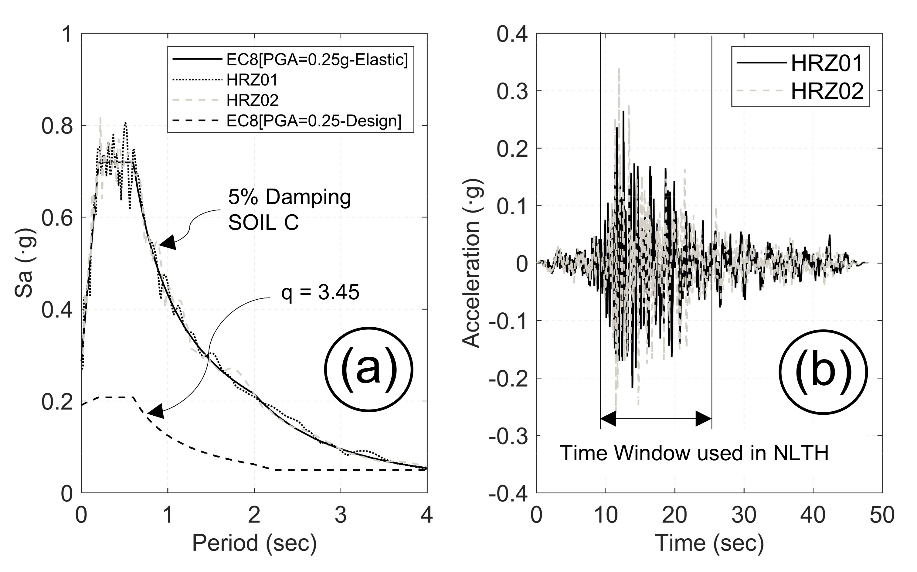
| MRSA | Design Response Spectrum with q = 3.45 according to Figure 11. | Modal Combination uses CQC rule. | [34] | 30% rule. |
| NLSA | Capacity Spectrum with 100 mm target displacement in both directions. | Multi-Modal according to [46]. | [18,36] | SRSS. |
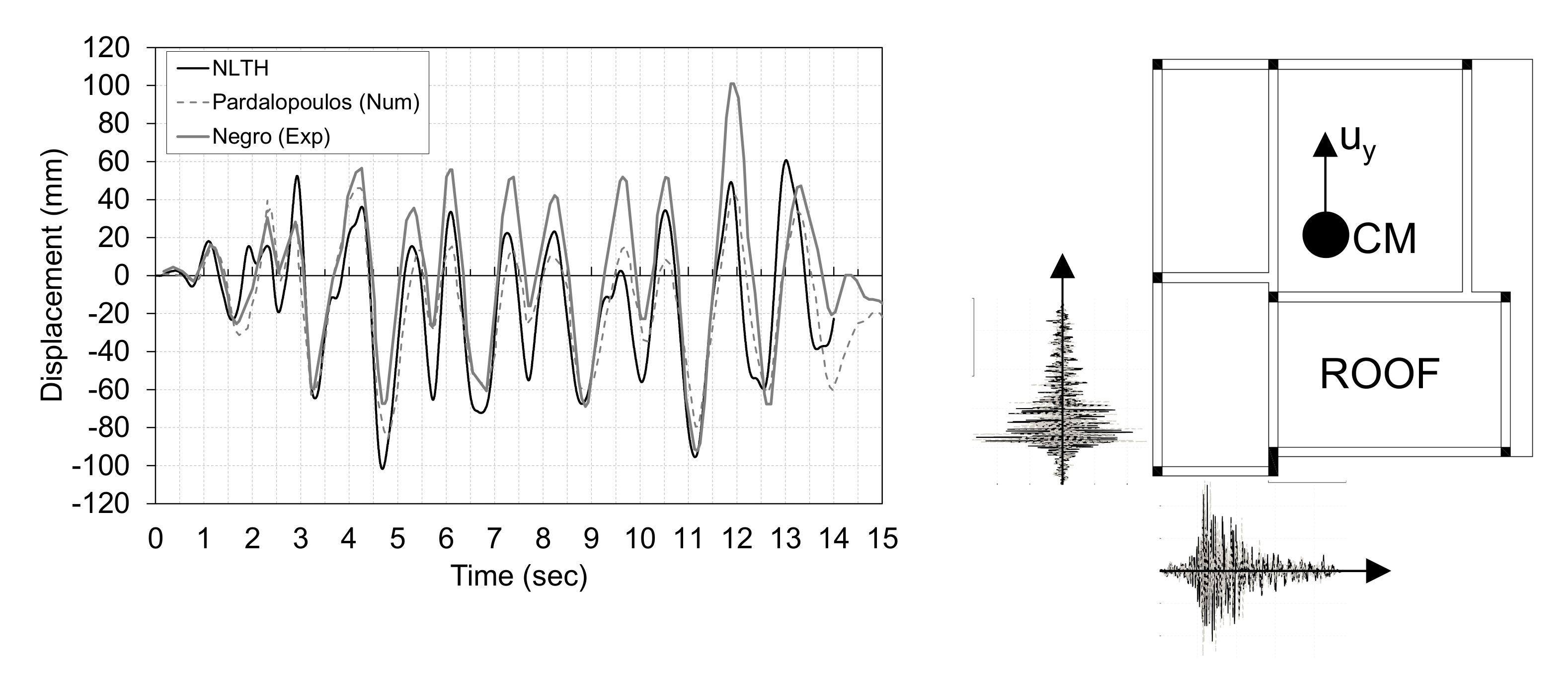
| NLTH | Herceg-Novi Accelerogram (PGA = 0.25 g) according to Figure 11 | Direct integration according to [47]. | [33] | Simultaneous inputs. |
| Author/Model | Ref. | |||||||||
|---|---|---|---|---|---|---|---|---|---|---|
| (s) | (%) | (%) | (s) | (%) | (%) | (s) | (%) | (%) | ||
| DiLudovico | [27] | 0.62 | 71.80 | 5.80 | 0.54 | 12.40 | 60.50 | 0.43 | 12.40 | 60.50 |
| Reynouard | [21] | 0.64 | - | - | 0.54 | - | - | 0.42 | - | - |
| Stratan | [36] | 0.57 | - | - | 0.48 | - | - | 0.39 | - | - |
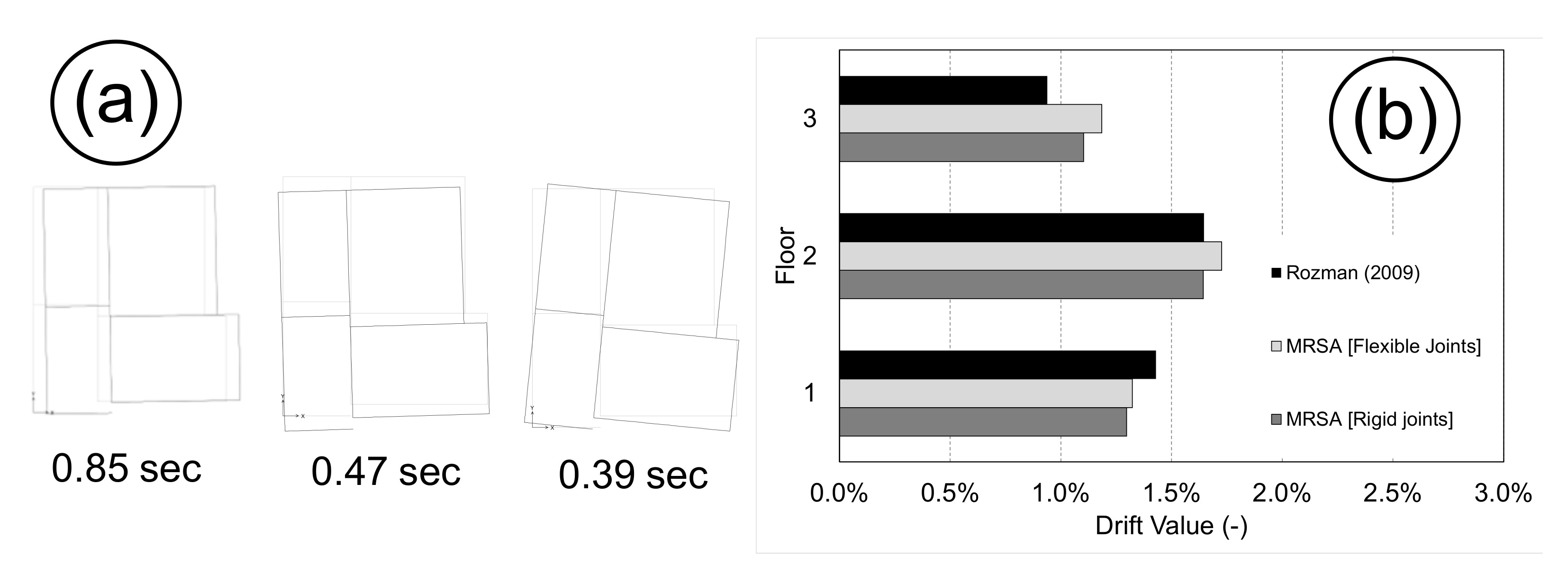
| Rozman | [34] | 0.80 | 69.00 | 4.80 | 0.69 | 15.60 | 47.80 | 0.58 | 2.70 | 30.30 |
| Negro (Experimental) | [19] | 0.84 | - | - | 0.78 | - | - | 0.67 | - | - |
| RIGID | This paper | 0.85 | 55.00 | 0.00 | 0.47 | 2.18 | 56.00 | 0.35 | 31.00 | 27.00 |
| FLEXI | This paper | 1.24 | 54.00 | 0.00 | 0.64 | 2.10 | 56.00 | 0.50 | 31.00 | 27.00 |
| Shear Strength | Shear Demand | ||||||||||||||
|---|---|---|---|---|---|---|---|---|---|---|---|---|---|---|---|
| min() | min() | max() | max() | ||||||||||||
| All the Values Are Expressed in MPa 0.5 | |||||||||||||||
| COL | FL | T-XZ | T-YZ | EC8 | ASCE41-17 | NZSEE2017 | MRSA | NLSA | NLTH | ||||||
| (a) | (b) | (c) | (d) | (e) | |||||||||||
| C8 | 1 | EXT | EXT | 0.03 | 0.471 | 0.498 | 0.498 | 0.397 | 0.397 | 0.531 | 0.517 | 0.703 | 0.700 | 0.515 | 0.778 |
| C9 | 1 | EXT-T | INT-T | 0.10 | 0.607 | 0.664 | 0.996 | 0.511 | 1.043 | 0.337 | 0.588 | 0.925 | 0.900 | 0.049 | 0.672 |
| C5 | 1 | EXT | EXT | 0.04 | 0.493 | 0.498 | 0.498 | 0.415 | 0.415 | 0.509 | 0.419 | 0.627 | 0.750 | 0.388 | 0.119 |
| C1 | 1 | INT-T | EXT-T | 0.16 | 0.701 | 0.996 | 0.664 | 1.143 | 0.591 | 0.618 | 0.303 | 0.884 | 1.161 | 0.920 | 0.683 |
| C2 | 1 | EXT | EXT | 0.11 | 0.626 | 0.498 | 0.498 | 0.528 | 0.528 | 0.408 | 0.364 | 1.074 | 0.728 | 0.709 | 0.525 |
| C4 | 1 | EXT | EXT | 0.21 | 0.767 | 0.498 | 0.498 | 0.647 | 0.647 | 0.309 | 0.444 | 0.771 | 0.769 | 0.039 | 0.241 |
| C7 | 1 | EXT | EXT | 0.08 | 0.571 | 0.498 | 0.498 | 0.481 | 0.481 | 0.378 | 0.562 | 0.768 | 0.556 | 0.075 | 0.241 |
| C6 | 1 | INT-T | EXT-T | 0.04 | 0.504 | 0.996 | 0.664 | 0.940 | 0.425 | 0.391 | 0.404 | 0.784 | 0.714 | 0.075 | 0.014 |
| C3 | 1 | EXT-T | INT-T | 0.31 | 0.884 | 0.664 | 0.996 | 0.747 | 1.352 | 0.231 | 0.673 | 1.521 | 0.886 | 0.369 | 0.718 |
| C8 | 2 | EXT | EXT | 0.01 | 0.433 | 0.498 | 0.498 | 0.364 | 0.364 | 0.429 | 0.486 | 0.512 | 0.553 | 0.508 | 0.905 |
| C9 | 2 | EXT-T | INT-T | 0.05 | 0.514 | 0.664 | 0.996 | 0.433 | 0.950 | 0.257 | 0.573 | 0.642 | 0.701 | 0.498 | 0.540 |
| C5 | 2 | EXT | EXT | 0.02 | 0.447 | 0.498 | 0.498 | 0.377 | 0.377 | 0.370 | 0.402 | 0.535 | 0.662 | 0.441 | 0.493 |
| C1 | 2 | INT-T | EXT-T | 0.08 | 0.574 | 0.996 | 0.664 | 1.009 | 0.484 | 0.462 | 0.304 | 0.684 | 0.838 | 0.553 | 0.536 |
| C2 | 2 | EXT | EXT | 0.05 | 0.524 | 0.498 | 0.498 | 0.441 | 0.441 | 0.296 | 0.327 | 0.800 | 0.664 | 0.477 | 0.569 |
| C4 | 2 | EXT | EXT | 0.11 | 0.614 | 0.498 | 0.498 | 0.518 | 0.518 | 0.241 | 0.393 | 0.563 | 0.695 | 0.500 | 0.397 |
| C7 | 2 | EXT | EXT | 0.04 | 0.491 | 0.498 | 0.498 | 0.414 | 0.414 | 0.304 | 0.497 | 0.728 | 0.406 | 0.463 | 0.783 |
| C6 | 2 | INT-T | EXT-T | 0.02 | 0.458 | 0.996 | 0.664 | 0.897 | 0.385 | 0.315 | 0.369 | 0.741 | 0.422 | 0.528 | 0.363 |
| C3 | 2 | EXT-T | INT-T | 0.16 | 0.695 | 0.664 | 0.996 | 0.587 | 1.138 | 0.183 | 0.663 | 1.050 | 0.499 | 0.374 | 0.664 |
| C8 | 3 | KNEE | KNEE | 0.00 | 0.404 | 0.332 | 0.332 | 0.340 | 0.340 | 0.173 | 0.257 | 0.498 | 0.234 | 0.195 | 0.217 |
| C9 | 3 | KNEE | KNEE | 0.00 | 0.404 | 0.332 | 0.332 | 0.340 | 0.340 | 0.106 | 0.241 | 0.268 | 0.265 | 0.170 | 0.208 |
| C5 | 3 | KNEE | KNEE | 0.00 | 0.404 | 0.332 | 0.332 | 0.340 | 0.340 | 0.140 | 0.188 | 0.249 | 0.306 | 0.358 | 0.228 |
| C1 | 3 | KNEE | KNEE | 0.00 | 0.404 | 0.332 | 0.332 | 0.340 | 0.340 | 0.170 | 0.140 | 0.279 | 0.332 | 0.250 | 0.210 |
| C2 | 3 | KNEE | KNEE | 0.00 | 0.404 | 0.332 | 0.332 | 0.340 | 0.340 | 0.118 | 0.151 | 0.332 | 0.263 | 0.143 | 0.123 |
| C4 | 3 | KNEE | KNEE | 0.00 | 0.404 | 0.332 | 0.332 | 0.340 | 0.340 | 0.104 | 0.156 | 0.239 | 0.260 | 0.105 | 0.259 |
| C7 | 3 | KNEE | KNEE | 0.00 | 0.404 | 0.332 | 0.332 | 0.340 | 0.340 | 0.133 | 0.230 | 0.562 | 0.166 | 0.168 | 0.235 |
| C6 | 3 | KNEE | KNEE | 0.00 | 0.404 | 0.332 | 0.332 | 0.340 | 0.340 | 0.144 | 0.229 | 0.702 | 0.177 | 0.141 | 0.224 |
| C3 | 3 | KNEE | KNEE | 0.00 | 0.404 | 0.332 | 0.332 | 0.340 | 0.340 | 0.080 | 0.323 | 0.384 | 0.174 | 0.224 | 0.201 |
Publisher’s Note: MDPI stays neutral with regard to jurisdictional claims in published maps and institutional affiliations. |
© 2022 by the authors. Licensee MDPI, Basel, Switzerland. This article is an open access article distributed under the terms and conditions of the Creative Commons Attribution (CC BY) license (https://creativecommons.org/licenses/by/4.0/).
Share and Cite
Marchisella, A.; Muciaccia, G. Comparative Assessment of Shear Demand for RC Beam-Column Joints under Earthquake Loading. Appl. Sci. 2022, 12, 7153. https://doi.org/10.3390/app12147153
Marchisella A, Muciaccia G. Comparative Assessment of Shear Demand for RC Beam-Column Joints under Earthquake Loading. Applied Sciences. 2022; 12(14):7153. https://doi.org/10.3390/app12147153
Chicago/Turabian StyleMarchisella, Angelo, and Giovanni Muciaccia. 2022. "Comparative Assessment of Shear Demand for RC Beam-Column Joints under Earthquake Loading" Applied Sciences 12, no. 14: 7153. https://doi.org/10.3390/app12147153
APA StyleMarchisella, A., & Muciaccia, G. (2022). Comparative Assessment of Shear Demand for RC Beam-Column Joints under Earthquake Loading. Applied Sciences, 12(14), 7153. https://doi.org/10.3390/app12147153