Estimating Full-Coverage PM_2.5 Concentrations Based on Himawari-8 and NAQPMS Data over Sichuan-Chongqing

Abstract

Fine particulate matter (PM_2.5) has attracted extensive attention due to its harmful effects on humans and the environment. The sparse ground-based air monitoring stations limit their application for scientific research, while aerosol optical depth (AOD) by remote sensing satellite technology retrieval can reflect air quality on a large scale and thus compensate for the shortcomings of ground-based measurements. In this study, the elaborate vertical-humidity method was used to estimate PM_2.5 with the spatial resolution 1 km and the temporal resolution 1 hour. For vertical correction, the scale height of aerosols (${\mathrm{H}}_{\mathrm{a}}$) was introduced based on the relationship between the visibility data and extinction coefficient of meteorological observations to correct the AOD of the Advance Himawari Imager (AHI) onboard the Himawari-8 satellite. The hygroscopic growth factor (f(RH)) was fitted site-by-site and month by month (1–12 months). Meanwhile, the spatial distribution of the fitted coefficients can be obtained by interpolation assuming that the aerosol properties vary smoothly on a regional scale. The inverse distance weighted (IDW) method was performed to construct the hygroscopic correction factor grid for humidity correction so as to estimate the PM_2.5 concentrations in Sichuan and Chongqing from 09:00 to 16:00 in 2017–2018. The results indicate that the correlation between “dry” extinction coefficient and PM_2.5 is slightly improved compared to the correlation between AOD and PM_2.5, with r coefficient values increasing from 0.12–0.45 to 0.32–0.69. The r of hour-by-hour verification is between 0.69 and 0.85, and the accuracy of the afternoon is higher than that of the morning. Due to the missing rate of AOD in the southwest is very high, this study utilized inverse variance weighting (IVW) gap-filling method combine satellite estimation PM_2.5 and the nested air-quality prediction modeling system (NAQPMS) simulation data to obtain the full-coverage hourly PM_2.5 concentration and analyze a pollution process in the fall and winter.

1. Introduction

The PM_2.5, as known as fine particulate matter, denotes particulate matter with an aerodynamic diameter less than 2.5 µm. PM_2.5 has raised significant public concerns over the past decades because of its adverse effects on human health [1]. Studies have shown that people who exposed to PM_2.5 for long periods of time are more likely to suffer from respiratory and cardiovascular diseases and even die prematurely [2,3]. Therefore, long-term continuous regional PM_2.5 concentration monitoring is important for the assessment of various haze impacts. To monitor air pollutants, China started to develop a ground-based monitoring network at the end of 2012, which has covered major cities by now. The ground-based monitoring network can grasp the real-time information of PM_2.5 concentration overtime at the observation sites with high accuracy, but it is difficult to support the assessment of regional haze impact due to the inability to accurately represent non-site regional concentrations. Meanwhile, the cost of site maintenance is high and the distribution is uneven with most located in urban centers. To overcome these limitations, the use of satellite remote sensing technology to derive the spatial and temporal distribution characteristics of PM_2.5 was proposed [4], due to its advantages such as wide spatial coverage and long time series [5,6].

The AOD retrieved by satellite is a measure of the integration of the extinction coefficient of the medium between satellite remote sensing and the ground in the vertical direction [7], which cannot directly represent the ground-level PM_2.5. Therefore, various methods have been proposed to represent the relationship between AOD and PM_2.5, and obtain the near-ground PM_2.5 concentration. Up to now, the main methods for estimating PM_2.5 concentration using AOD are scale factor methods, semi-empirical formula methods, statistical model methods, and machine learning methods. The scale factor method simulates the scale coefficient between PM_2.5 and AOD by atmospheric radiative transfer model and then multiplies the coefficient by the AOD obtained from satellite retrieval, which does not involve ground-based monitoring data and is conducive to estimating PM_2.5 concentration during the period when there is no ground-based monitoring station, but the estimation accuracy is low [8,9,10]. The semi-empirical formula method is based on the physical properties between AOD and PM_2.5 such as humidity and vertical profile features of AOD [11,12,13,14,15]. However, it is difficult to fully express the relationship between PM_2.5 and AOD by a simple function due to its complex physical mechanism, while some parameters in the semi-empirical formula are not easily accessible, which limits the extension of this method. The statistical model method evolved from the initial linear model (e.g., linear mixed-effect regression, LME) [16,17] to the nonlinear regression model (e.g., generalized additive model, GAM; geographically and temporally weighted regression, GTWR) [18,19,20]. Some researches improve the accuracy of the model by introducing meteorology, topography, land use and other relevant parameters [21,22], but the nonlinear relationship between the factors still cannot be fully expressed. Machine learning algorithms have significant advantages over statistical models for classification and prediction [23], and a variety of models are widely used for PM_2.5 estimation, e.g., random forest (RF) [24,25], Deep Neural Networks (DNN) [26,27], Capsule Networks (CapsNet) [28], space-time extremely randomized trees (STEM) [29]. Machine learning methods have the advantage of expressing nonlinear relationships between large data and achieve excellent results in estimation accuracy compared with other methods but ignore the physical characteristics between AOD and PM_2.5. As the relationship between AOD and PM_2.5 varies greatly from region to region, moment to moment, and season to season [30,31], most studies that used a single machine learning method to estimate PM_2.5 concentrations in a large area have some shortcomings in spatial distribution. Meanwhile, the accuracy of the estimation using machine learning methods is related to the training samples.

Meanwhile, there is still a huge challenge in estimating regional PM_2.5 concentrations using AOD, which is missing AOD retrievals caused by cloud cover and bright surfaces (desert or snow) [32,33]. Different methods are proposed for addressing missing AOD retrievals, such as kriging interpolation [34], machine learning methods to combine chemical transport models such as the Community Multi-scale Air Quality Model (CMAQ), Modern-Era Retrospective Analysis for Research and Applications-version 2 (MERRA-2) to simulate AOD or PM_2.5 with complete spatial and temporal coverage. For example, Sun et al. combined Multi-angle Implementation of Atmospheric Correction (MAIAC) AOD, AHI AOD, and meteorological data to obtain 24 h full-coverage PM_2.5 concentrations in Beijing [35]. Li et al. used residual networks for the downscaling fusion of MERRA-2 and MAIAC AOD to obtain full-coverage of PM_2.5 concentrations in the California [36]. Chen et al. used AQUA and TERRA AOD to perform linear regression firstly, and then combined with Copernicus Atmosphere Monitoring Service (CAMS) AOD, using a self-adaptive deep neural network (SADNN) to estimate regional full-coverage PM_2.5 in China [37]. Bai et al. performed ten different fusion strategies for comparison to obtaining full-coverage PM_2.5 concentrations using the classical RF model [38].

Due to the unique climatic conditions in the Sichuan and Chongqing regions, where the air pollution is heavier but with more cloud coverage in autumn and winter, and less cloud coverage but relatively better air quality in spring and summer. As well know, machine learning method is relation with training samples, the training samples in the special area of the study may not truly represent the distribution of PM_2.5 long-time series. Thus, we proposed the elaborate Vertical-Humidity correction method to estimate PM_2.5 concentrations in areas of Sichuan and Chongqing (the scope of the study mainly includes the Sichuan area except Ganzi, Aba, Liangshan, and Panzhihua, and the main urban area of Chongqing). Meanwhile, to make up for the missing data of PM_2.5 retrieved by satellite, we combine satellite and NAQPMS data to obtain full-coverage PM_2.5 concentration over Sichuan and Chongqing. The main research of this study is as follows:

(1)

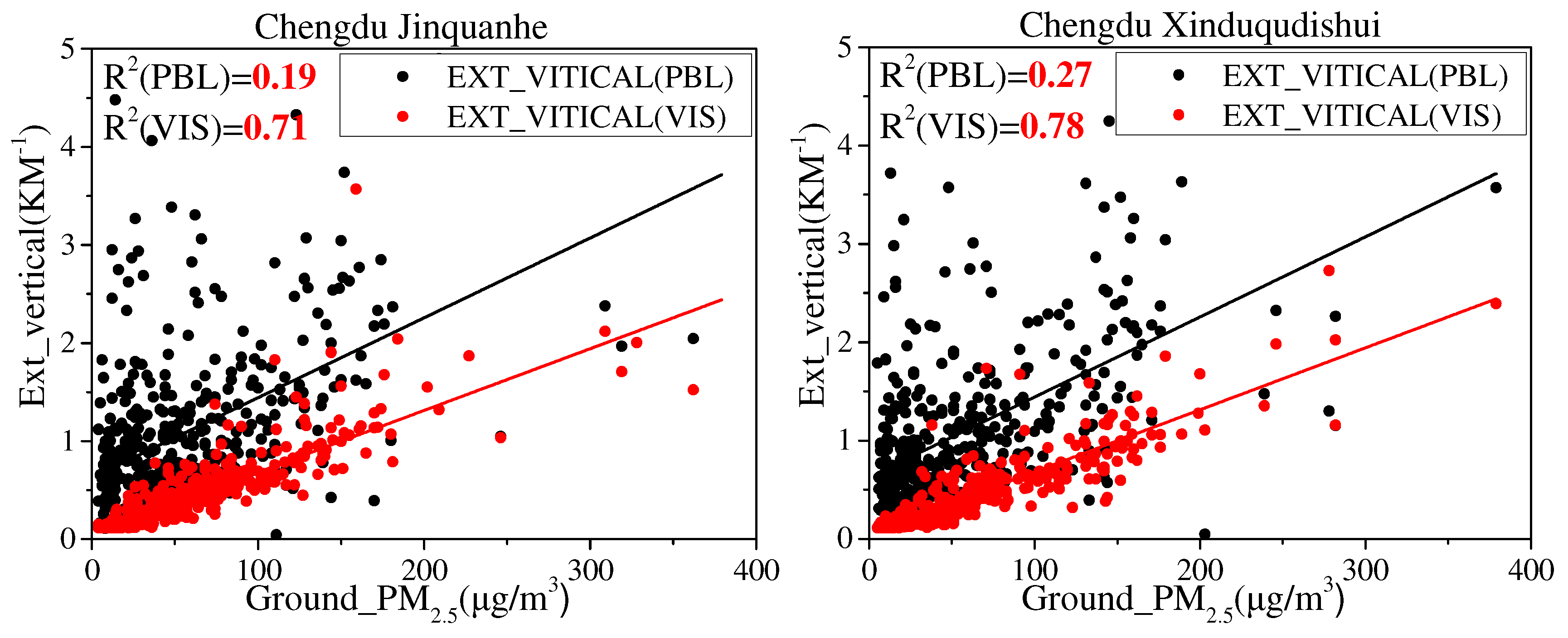
Considering the complex topography and meteorological conditions in Sichuan and Chongqing, the scale height of aerosols (${\mathrm{H}}_{\mathrm{a}}$) was introduced for the vertical correction of regional AOD. For humidity correction, five different stations were selected for the analysis of the fitted curves and f(90%), and the results showed that the hygroscopic correction factors varied greatly in different months and stations, so the data in the study area were fitted site by site and month by month to construct a grid of hygroscopic correction factors.

(2)

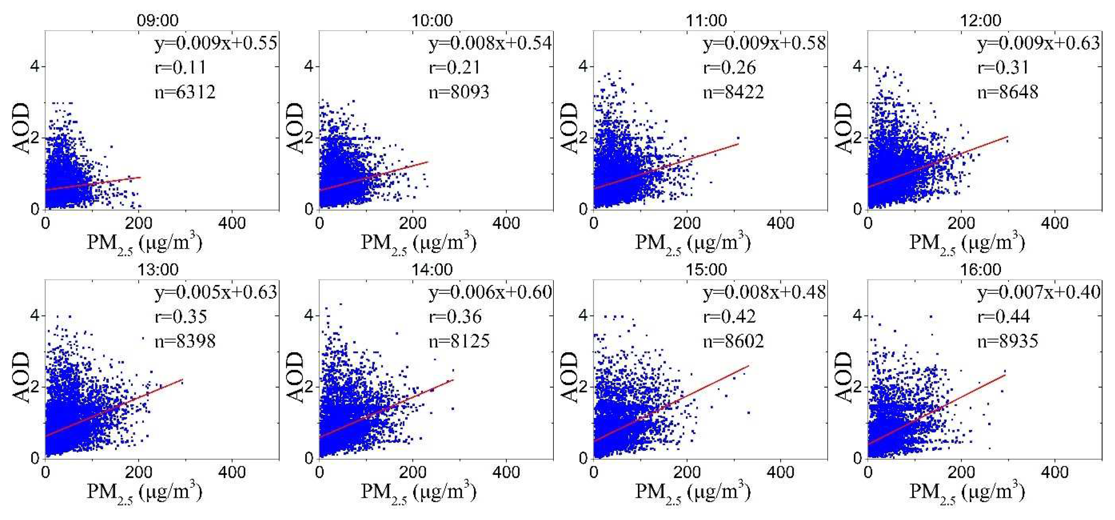
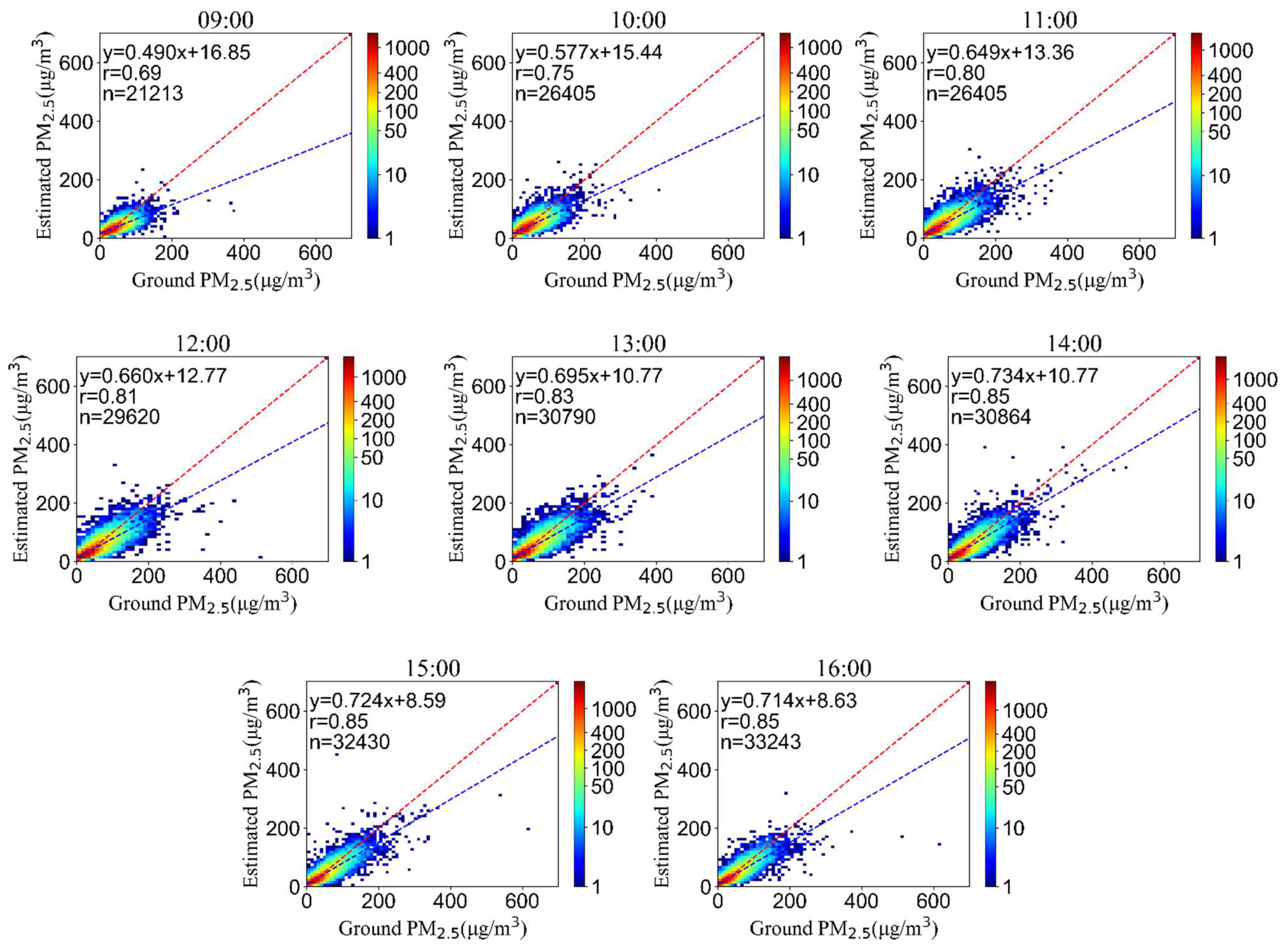
The hourly PM_2.5 concentrations in the study area from 09:00 to 16:00 were estimated using the AHI AOD data based on the constructed hygroscopic correction factors grid, and the accuracy was verified.

(3)

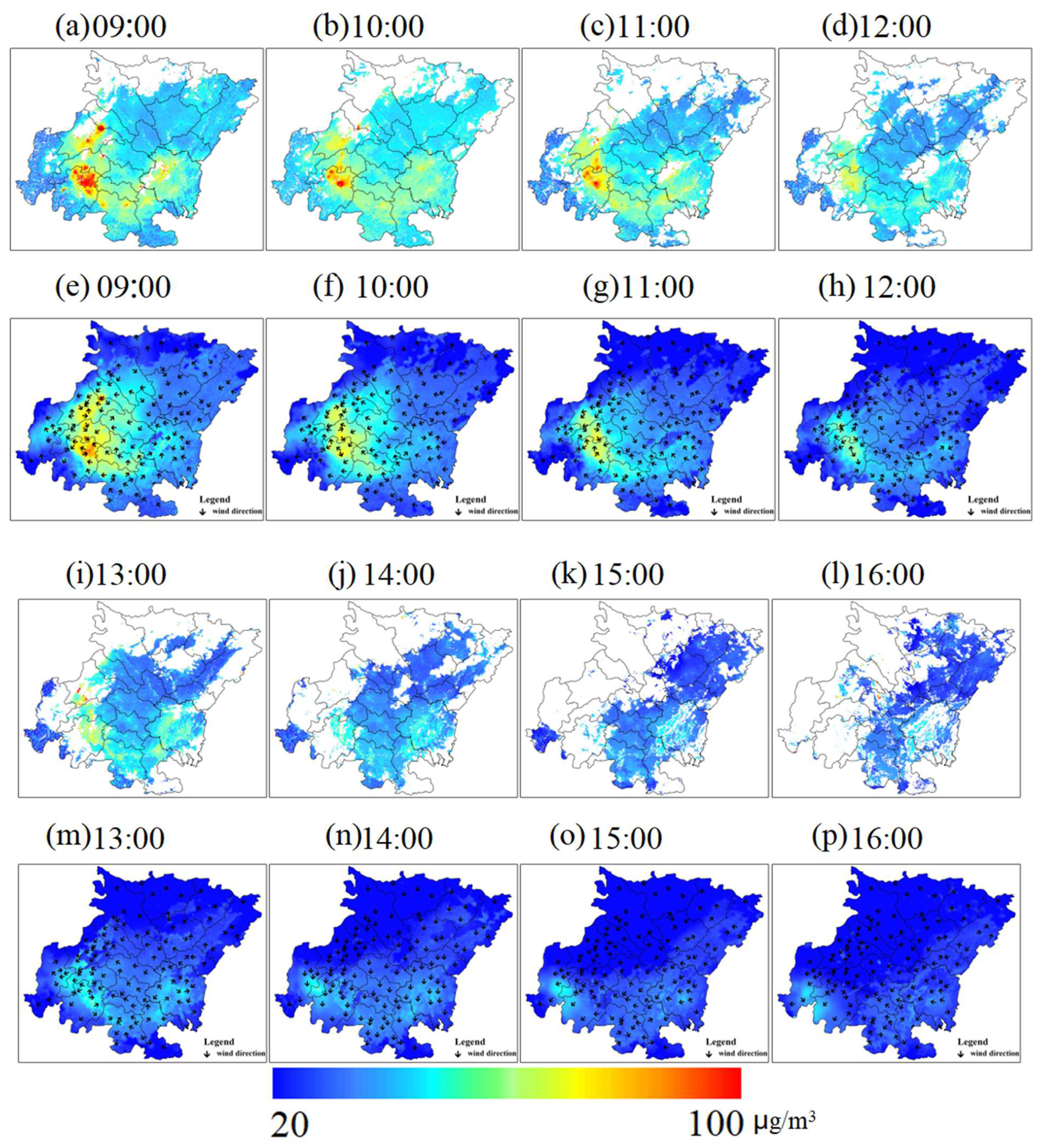
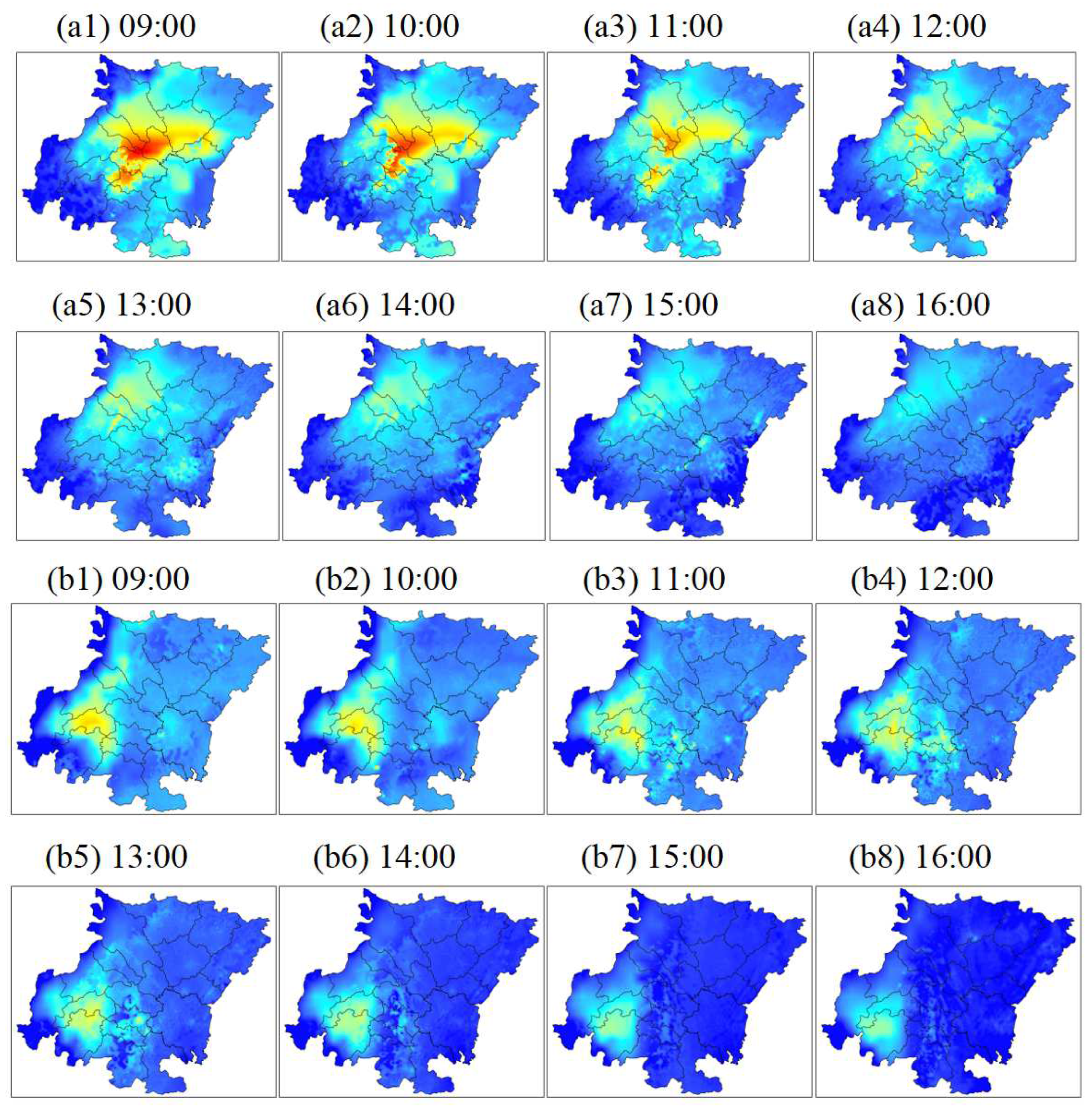
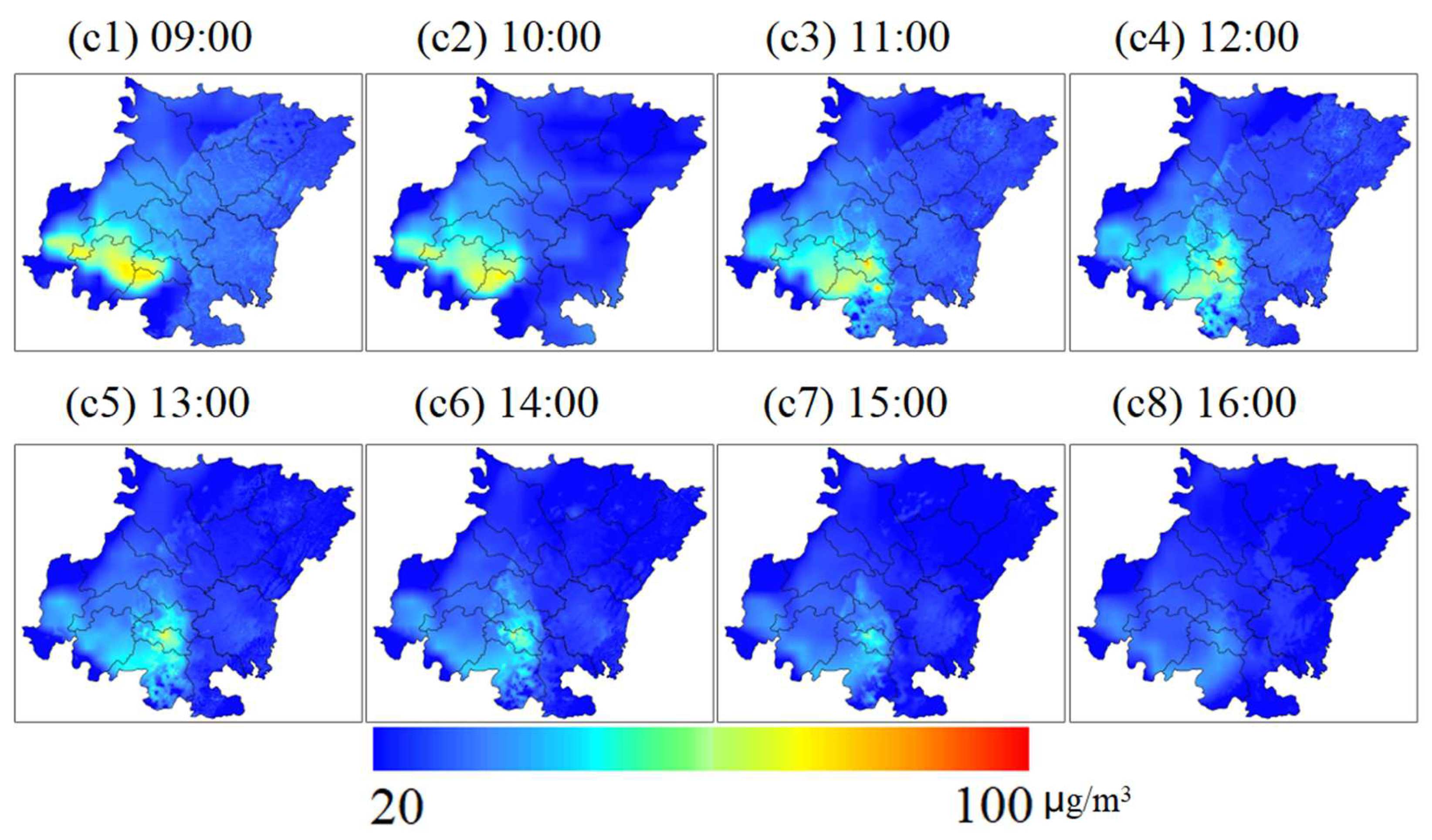
Considering the frequent cloud coverage in Sichuan and Chongqing regions and the existence of gaps in the satellite retrieval PM_2.5, we adopt inverse variance weighting (IVW) for effective fusion with the help of NAQPMS data to finally obtain PM_2.5 concentrations with seamless coverage and effectively analyze the processes of pollutant aggregation, migration, and dissipation in this place.

2. Materials and Methods

The study area we selected mainly includes Sichuan Province (except Ganzi, Aba, Liangshan, and Panzhihua) and the main urban area of Chongqing (Figure 1), which located in southwest China, with regional elevations ranging from 400–5000 m [39]. The study area is influenced by the Qinghai-Tibet Plateau to form high humidity and low wind speed atmospheric conditions, which are not conducive to pollution transmission and are prone to haze with the wide range and long duration leading to heavy pollution. Additionally, the population of the region is about 100 million, and a large amount of industrial, traffic, and anthropogenic emissions of pollutants leads to frequent heavy pollution weather [40].

2.1. Data

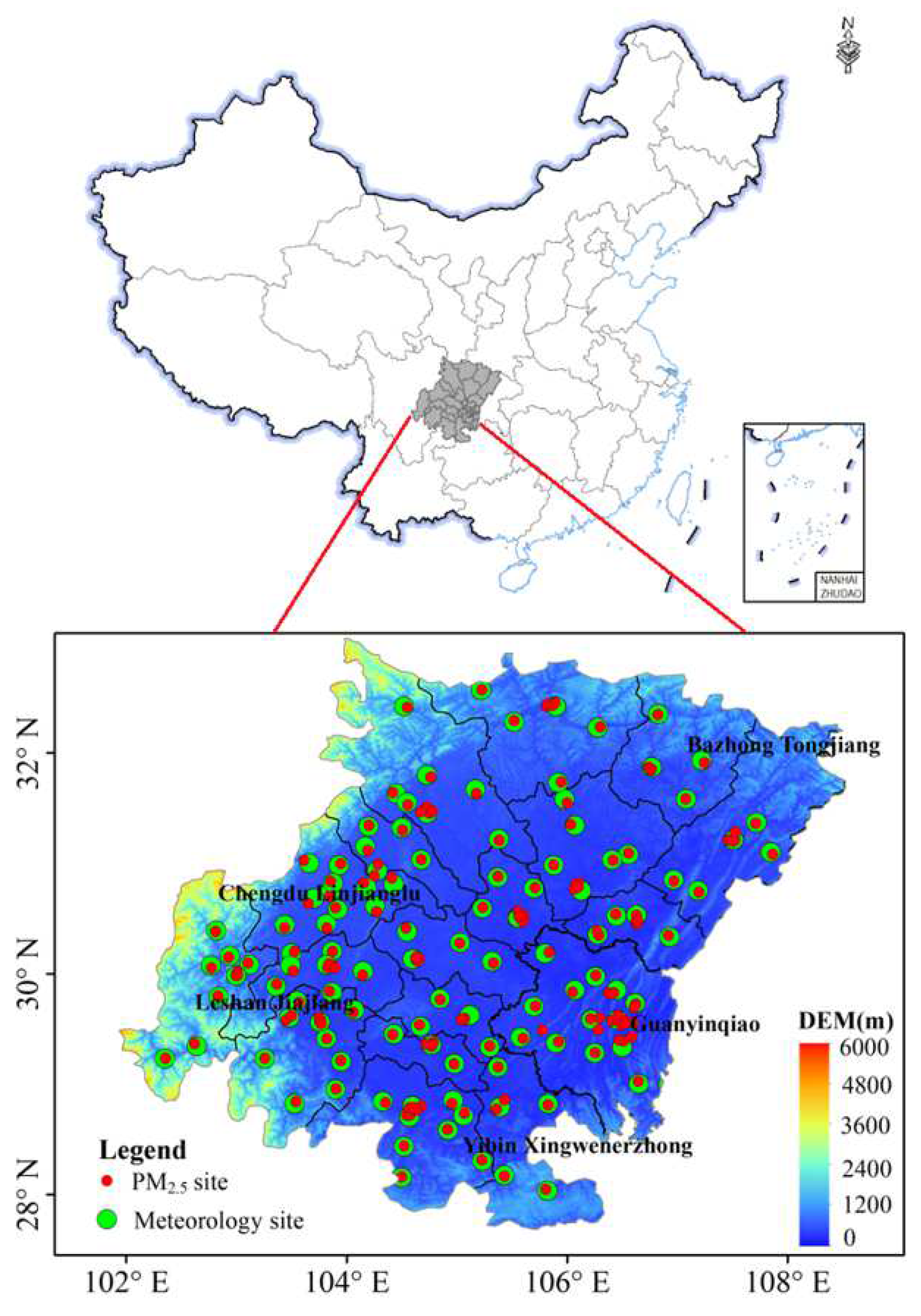
2.1.1. Ground-Level PM_2.5 Measurements

Ground measured hourly PM_2.5 concentration data in 2017 and 2018 were obtained from the China National Environmental Monitoring Center (CNEMC) (http://106.37.208.233:20035/, accessed on 12 June 2022), Department of Ecology and Environment of Sichuan Province, and Chongqing Environmental Monitoring Center, including CNEMC stations, Sichuan stations, and Chongqing stations. For every three hours of data, PM_2.5 concentration values below the 3% quantile or above the 97% quantile are not included in the calculation.

2.1.2. Himawari-8 AHI/AOD Data

Himawari-8 is a second-generation geostationary meteorological satellite of Japan Meteorological Agency (JMA), which was successfully launched in October 2014 and officially put into operation in July 2015. Himawari-8 carries an AHI sensor with 16 observation channels, which includes 3 visible channels, 3 near-infrared channels, and 10 infrared channels, of which the resolution of visible channels can reach 0.5 km, and the resolution of near-infrared and infrared channels can reach 1~2 km. This study used the AOD by the dark target algorithm retrieval with a spatial resolution of 1 km and a temporal resolution of 1 h; please refer to the literature for the detailed retrieval algorithm [41].

2.1.3. Meteorological Data

The meteorological data were obtained from China Meteorological Data Service Centre with a temporal resolution of 1 h, and the two main parameters utilized were visibility (VIS) and relative humidity (RH). To reduce the experimental error, the data were pre-processed as follows. (1) If the ratio of the visibility data of the current day to the data of the previous day and the next day was less than 1/3 in three consecutive days, the visibility data of that day were deleted [42]. (2) Relative humidity values greater than 98% were not involved in the statistical study. (3) To avoid affecting the aerosol hygroscopic growth fitting results, when matching environmental monitoring station data and meteorological station data, if the distance between two stations was greater than 10 km, they were not involved in the statistical study.

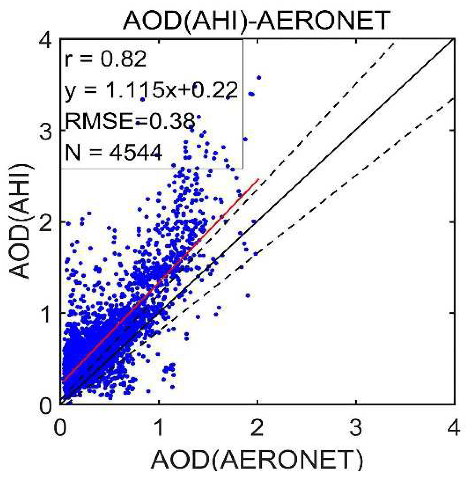
2.1.4. Aerosol Robotic Network (AERONET) Data

To verify the accuracy of the AHI AOD in the retrieval of this study, we downloaded the AERONET [43] level 2.0 data of 2017 and 2018 at six stations: Bamboo (25.19° N, 121.54° E), Hong Kong PolyU (22.3° N, 114.18° E), Hong Kong Sheung (22.48° N, 114.12° E), Beijing CAMS (39.93° N,116.32° E), Xiang He (39.75° N, 116.96° E), and Beijing (39.98° N, 116.38° E). The AERONET AODs were interpolated using 440 nm and 675 nm with the help of Angstrom exponential to be consistent with the AHI AOD 550 μm band [44]. During the validation process, to ensure consistency in space and time, the average value of 3×3 images was calculated with AERONET sites as the center, and the average value of AERONET AOD before and after half an hour of satellite transit time was calculated, with a total of 4544 validation data. The validation comparison scatter plot is shown in Figure 2, with a high correlation coefficient value of r = 0.82 and a fit slope close to 1, RMSE = 0.38.

2.1.5. Nested Air Quality Prediction Modeling System (NAQPMS) Data

The simulated PM_2.5 data used in this study were obtained from the Nested Air Quality Prediction Modeling System (NAQPMS); the NAQPMS is a multiscale air-quality model developed by the Institute of Atmospheric Physics, Chinese Academy of Sciences. The NAQPMS uses a new generation of mesoscale Weather Research and Forecast (WRF) models with a resolution of 1–30 km developed by the National Center for Environmental Prediction (NCEP), the National Center for Atmospheric Research (NCAR), and other research institutions and universities [45,46]. The NAQPMS can simulate atmospheric trace gases (e.g., O₃, NO_X, SO₂, CO) and atmospheric aerosol components (e.g., sand, sea salt, sulfate, nitrate, ammonium, and carbon-containing aerosols). It has been widely used in the study of the development mechanism and transport deposition process of sand, dust, acid rain, ozone, and particulate pollution, as well as the forecast and prediction of urban air quality [47]. To be consistent with the AHI AOD resolution, the NAQPMS was resampled to 1 km by the nearest neighbor method.

2.2. Methods

AOD represents the sum of the extinction capacity of all aerosol particles in the vertical column of the atmosphere. To obtain near-ground PM_2.5, not only the near-ground extinction coefficient needs to be revised from the vertical extinction coefficient, but also the hygroscopic properties of the particles should be considered. However, the hygroscopic properties of aerosol particles vary greatly in different seasons and regions, so this study fitted the hygroscopic growth factors month by month and site by site and constructed a grid of hygroscopic correction factors by using the IDW method.

2.2.1. Vertical Correction

Assuming that the extinction coefficient of the aerosol shows a negative exponential decay in the vertical direction, the AOD can be expressed as:

$$\mathrm{AOD}={{\displaystyle \int }}_0^{\infty }{\mathsf{\sigma }}_{\mathrm{a}}\left(\mathsf{\lambda }\right)\times {\mathrm{e}}^{-\frac{\mathrm{z}}{{\mathrm{H}}_{\mathrm{a}}}}\mathrm{dz}={\mathsf{\sigma }}_{\mathrm{a}}\left(\mathsf{\lambda }\right)\times {\mathrm{H}}_{\mathrm{a}}$$

(1)

where $\mathsf{\lambda } =550$ nm, $\mathrm{z}$ denotes the height in the vertical direction, and ${\mathsf{\sigma }}_{\mathrm{a}}\left(\mathsf{\lambda }\right)$ is the near-ground extinction coefficient, which unit is m⁻¹. ${\mathrm{H}}_{\mathrm{a}}$ is the scale height of aerosols. ${\mathrm{H}}_{\mathrm{a}}$ can be approximately replaced by the boundary [48], the unit of which is m.

According to Koschmieder’s law [49,50,51], the near-ground extinction coefficient ${\mathsf{\sigma }}_{\mathrm{a}}\left(\mathsf{\lambda }\right)$ can be expressed by Equation (2):

$${\mathsf{\sigma }}_{\mathrm{a}}\left(\mathsf{\lambda }\right)=\frac{3.912}{\mathrm{vis}}-\frac{32{\mathsf{\pi }}^3{\left(\mathrm{n}-1\right)}^2}{3{\mathrm{N}\mathsf{\lambda }}^4}$$

(2)

where n denotes the atmospheric refractive index, and N denotes the molecular number density. At sea level, n − 1 = 293 × 10⁻⁶, N = 266 × 10⁻¹⁹ cm⁻³.

Therefore, the visibility provided by the meteorological station can be used to calculate the near-ground extinction coefficient ${\mathsf{\sigma }}_{\mathrm{a}}\left(\mathsf{\lambda }\right)$ and thus the corresponding ${\mathrm{H}}_{\mathrm{a}}$. Assuming that the variation of ${\mathrm{H}}_{\mathrm{a}}$ is small within a certain range, this study uses IDW to interpolate ${\mathrm{H}}_{\mathrm{a}}$ distribution to 1 km in the study area.

2.2.2. Relativity Correction

Based on the Mie scattering theory [11,48], the near-ground extinction coefficient of aerosols ${\mathsf{\sigma }}_{\mathrm{a}}\left(\mathsf{\lambda }\right)$ can also be expressed as:

$${\mathsf{\sigma }}_{\mathrm{a}}\left(\mathsf{\lambda }\right)=\frac{3\langle {\mathrm{Q}}_{\mathrm{ext}}\rangle }{4{\mathrm{r}}_{\mathrm{eff}}\mathsf{\rho }}·{\mathrm{PM}}_{\mathrm{x}}$$

(3)

where $\langle {\mathrm{Q}}_{\mathrm{ext}}\rangle$ denotes the scattering efficiency of normalized particles, ${\mathrm{r}}_{\mathrm{eff}}$ denotes the effective radius of the particle, $\mathsf{\rho }$ denotes the average density of particles, $\mathrm{PMx}$ denotes the mass concentration of aerosol, and all parameters are influenced by relative humidity. Assuming that the particles, particle spectrum, and density of the aerosol remain relatively constant, $\langle {\mathrm{Q}}_{\mathrm{ext}}\rangle$, ${\mathrm{r}}_{\mathrm{eff}}$, and $\mathsf{\rho }$ can be viewed as constants so that there is a certain positive relationship between ${\mathsf{\sigma }}_{\mathrm{a}}\left(\mathsf{\lambda }\right)$ and $\mathrm{PMx}$. According to the average mass extinction rate defined by Wang [11].

$${\mathrm{E}}_{\mathrm{ext}}=\frac{{\mathsf{\sigma }}_{\mathrm{a}}\left(\mathsf{\lambda }\right)}{{\mathrm{PM}}_{\mathrm{x}}}\approx {\mathrm{E}}_{\mathrm{ext}}\left(\mathrm{RH}\right)$$

(4)

Since the fine particulate matter is the main contributor to aerosol extinction, here, $\mathrm{PMx}$ refers to particulate matter with a particle radius less than 2.5 μm, and ${\mathrm{E}}_{\mathrm{ext}}\left(\mathrm{RH}\right)$ describes the average state of the extinction ability of particles with different properties. To quantitatively describe the hygroscopic growth characteristics of ${\mathrm{E}}_{\mathrm{ext}}\left(\mathrm{RH}\right)$, the extinction hygroscopic growth factor of the average mass extinction rate $\mathrm{f}\left(\mathrm{RH}\right)$ can be expressed as

$$\mathrm{f}\left(\mathrm{RH}\right)=\frac{{\mathrm{E}}_{\mathrm{ext}}\left(\mathrm{RH}\right)}{{\mathrm{E}}_{\mathrm{dry}}}$$

(5)

where ${\mathrm{E}}_{\mathrm{dry}}$ denotes the average mass extinction rate under dry conditions (RH = 40%). According to the Kotchenruther’s research [52], ${\mathrm{E}}_{\mathrm{ext}}\left(\mathrm{RH}\right)$ can be represented by Equation (6),

$${\mathrm{E}}_{\mathrm{ext}}\left(\mathrm{RH}\right)=\mathrm{a}+ \mathrm{b}\times {\left(\frac{\mathrm{RH}}{100}\right)}^{\mathrm{c}}$$

(6)

where a, b, and c are coefficients fitted with RH variation, depending on the aerosol physicochemical properties. According to the above equations, the expression of PM_2.5 can be obtained as follows:

$${\mathrm{PM}}_{2.5}=\frac{{\mathsf{\sigma }}_{\mathrm{a}}\left(\mathsf{\lambda }\right)}{{\mathrm{E}}_{\mathrm{ext}}\left(\mathrm{RH}\right)}=\frac{\frac{\mathrm{AOD}}{{\mathrm{H}}_{\mathrm{a}}}}{\left(\mathrm{a}+\mathrm{b}\times {\left(\frac{\mathrm{RH}}{100}\right)}^{\mathrm{c}}\right)\times {\mathrm{E}}_{\mathrm{dry}}}$$

(7)

Since fine particles can stay in the atmosphere for days or even weeks and can be well mixed in the atmosphere and transported over long distances to other regions, the spatial distribution of the fitted coefficients a, b, and c can be obtained by interpolation, assuming that the aerosol properties vary smoothly on a regional scale. Subsequently, assuming that the regional relative humidity varies smoothly, the distribution of relative humidity in the study area can be obtained by IDW interpolation. Finally, the PM_2.5 concentration value of each pixel can be calculated based on the AOD, ${\mathrm{H}}_{\mathrm{a}}$, relative humidity, a, b, and c in the study area.

2.2.3. IVW Fusion Method

To fill the gap in PM_2.5 estimation by satellite, we used the inverse variance weighting method (IVW), which is based on the difference between PM_2.5 estimated by satellite (NAQPMS) and ground-based PM_2.5 data, to fuse satellite data and NAQPMS data. Since the dispersion of the variance is related to the quality of the estimation (or simulation) results, by calculating the variance of the corresponding data pair, a lower weight is assigned when the variance between the estimated (simulated) results and the ground-based data is large, and when the variance is small, a higher weight is assigned [53]. The IVW method is expressed as follows:

$${\mathrm{PM}}_{\mathrm{f}}=\frac{\frac{{\mathrm{PM}}_{\mathrm{st}-\mathrm{f}}}{{\mathrm{Var}}_{\mathrm{stm}}}+\frac{{\mathrm{PM}}_{\mathrm{model}-\mathrm{f}}}{{\mathrm{Var}}_{\mathrm{modelm}}}}{\frac{1}{{\mathrm{Var}}_{\mathrm{stm}}}+\frac{1}{{\mathrm{Var}}_{\mathrm{modelm}}}}$$

(8)

where ${\mathrm{PM}}_{\mathrm{st}-\mathrm{f}}$ and ${\mathrm{PM}}_{\mathrm{model}-\mathrm{f}}$ denote PM_2.5 of satellite estimation and NAQPMS simulation. ${\mathrm{Var}}_{\mathrm{stm}}$ (${\mathrm{Var}}_{\mathrm{modelm}}$) is the variance of the difference between the satellite estimation (NAQPMS simulation) and the ground-based PM_2.5. ${\mathrm{PM}}_{\mathrm{f}}$ is PM_2.5 concentration after fusion.

This study fused the satellite estimated PM_2.5 with the NAQPMS simulation results to obtain spatially full-coverage PM_2.5 distribution.

3. Results

3.1. The Fitting Result of $E_{ext}\left(RH\right)$ and Statists Analysis of $f\left(RH\right)$

In this study, ${\mathrm{E}}_{\mathrm{ext}}\left(\mathrm{RH}\right)$ fitting results for five different urban sites were selected for analysis, which are Chengdu Lingjianglu (built-up area), Leshan Jiajiangxian (near the river), Yibin Xingwenerzhong (densely vegetated area), Bazhong Tongjiangzhongxue (near the river), and Chongqing Guanyinqiao (commercial area), and the fitting results are shown in Figure 3 and Figures S1–S4. In general, (1) the fitting ability of the model was strong at all five stations, with r around 0.9 at the stations of Leshan Jiajiang, Yibin Xingwen, and Chongqing Guanyinqiao; only in February, June, and December was the r less than 0.8 at the station of Bazhong Tongjiang, and the r was less than 0.8 at the station of Chengdu Linjiang only in July and August. (2) While the RH value is small, ${\mathrm{E}}_{\mathrm{ext}}\left(\mathrm{RH}\right)$ grows slowly with RH, but the fitted curve is flat while RH > 80%, and the ${\mathrm{E}}_{\mathrm{ext}}\left(\mathrm{RH}\right)$ shows a fast-rising trend.

The fitting results of the five stations have obvious differences: the fitted curve of the Chengdu Lingjianglu station is basically the same from January to December and shows a slow rise when the relative humidity is higher, indicating that the aerosol hygroscopic growth characteristics of this station are weak, and its aerosol sources and environmental conditions vary less with the season [54], which may be related to the location of the selected station in a built-up area. The differences in hygroscopic growth characteristics between the months are large at Leshan Jiajiang and Bazhong Tongjiang, which are located close to the river. The fitted curve of Leshan Jiajiang shows a slow rise from January to May but a sharp rise from June to October, indicating that the hygroscopic growth characteristics vary greatly with the seasons, and there is almost no relative humidity less than 40% in July and August. For Bazhong Tongjiang, the fitted curve shows a sharp and steep rise in all 12 months. The hygroscopic growth characteristics of Yibin Xingwen, located in a densely vegetated area, and Chongqing Guanyinqiao Station, located in a commercial area, are relatively similar, where the fitted curves both show a slow rise from January to December with no obvious deliquescence.

Using Equation (5), f(90%) from January to December was calculated for Chengdu Linjianglu, Leshan Jiajiangxian, Yibin Xingwenerzhong, Bazhong Tongjiangzhongxue, and Chongqing Guanyinqiao, respectively. The corresponding f(90%) could not be calculated because of the missing value of relative humidity less than 40% in December at Chongqing Guanyinqiao station and in July and August at Leshan Jiajiang station, as shown in

Table 1. Hygroscopic growth ability of f (90%) at Chengdu Linjianglu, Leshan Jiajiangxian, Yibin Xingwenerzhong, Bazhong Tongjiangzhongxue, and Chongqing Guanyinqiao.

Month	Chengdu Linjianglu	Yibin Xingwenerzhong	Leshan Jiajiangxian	Bazhong Tongjiang	Chongqing Guanyinqiao
January	1.85	1.62	3.64	1.51	2.46
February	1.58	1.70	5.02	1.65	2.51
March	1.58	2.38	4.92	1.65	2.67
April	1.57	3.52	4.59	1.45	4.85
May	1.47	2.66	4.03	1.33	3.94
June	1.70	1.92	2.44	1.46	3.78
July	2.08	1.93	-	1.85	4.78
August	2.52	1.83	-	1.21	4.64
September	1.99	2.38	3.22	1.19	5.35
October	1.20	3.52	1.13	1.41	3.27
November	1.61	3.91	3.26	1.62	5.34
December	2.22	2.57	2.68	2.14	-

. Comparison of different stations showed that the hygroscopic growth factors varied widely among stations, the variation of f(90%) at the same site in different months was large. There are 3.91 in November and 1.70 in February at Yibin Xingwenerzhong, and 5.02 in February and 1.13 in October at Leshan Jiajiangxian. The f(90%) of Chongqing Guanyinqiao is the highest (low) at 5.35 (2.46). There are small variations both Chengdu Linjianglu and Bazhong Tongjiangzhongxue stations. The f(90%) at Chongqing Guanyinqiao and Leshan Jiajiangxian stations are significantly higher than other stations, which the reason is that the main source of aerosols in commercial areas is secondary pollutants (such as sulfates) from vehicle emissions, which are water-soluble ions with strong hygroscopic properties. Leshan Jiajiangxian site is located between the built-up area and the river, and the aerosol is relatively complex.

3.2. Vertical and Humidity Correction on AOD

To verify that the dry extinction coefficient of AOD after vertical and humidity corrections (${\mathsf{\sigma }}_{\mathrm{dry}}$) is useful for estimating PM_2.5 concentration, the scatter plots of AOD&PM_2.5 from 09:00 to 16:00 (Beijing time) and the ${\mathsf{\sigma }}_{\mathrm{dry}}$ and PM_2.5 are shown in Figure 4 and Figure 5. According to Figure 4, the correlation coefficient between AOD and PM_2.5 increased by hours, and the correlation coefficient ranged from 0.11 to 0.44 (the lowest correlation r = 0.11 at 9:00 and the highest correlation r = 0.44 at 16:00). The correlation between the ${\mathsf{\sigma }}_{\mathrm{dry}}$ and PM_2.5 was significantly improved (Figure 5), with the highest correlation r = 0.68 at 15:00. Comparison of Figure 4 and Figure 5 shows that the correlation between the ${\mathsf{\sigma }}_{\mathrm{dry}}$ and PM_2.5 after the vertical and humidity corrections is significantly improved, which is beneficial to the estimation of PM_2.5 concentration.

3.3. The PM_2.5 of Satellite Estimation Validation

The comparison of Figure 4 and Figure 5 shows that the correlation between ${\mathsf{\sigma }}_{\mathrm{dry}}$ and PM_2.5 is significantly improved after the vertical and humidity corrections compared to that between AOD and PM_2.5, and the correlation coefficient increases from 0.11–0.44 to 0.28–0.68. The mass concentration of near-ground PM_2.5 was estimated using Equation (8), and the hour-by-hour density scatter plots of satellite estimates against ground-based observations are shown in Figure 6, where the red dashed line is the 1:1 line, and the blue dashed line is the fitted line. According to Figure 6 the correlations are all high in general, but the correlation coefficient varies more from 09:00 to 16:00 (0.69–0.85), and the correlation is significantly higher in the afternoon than in the morning, the variation of which is consistent with the study of Xu [30]. This may be caused by the following two reasons: (1) in the morning hours, when the solar azimuth is larger and the atmospheric water vapor content is higher, the sunlight passes through a longer atmospheric path to reach the ground, which affects the accuracy of the AOD retrieval, and thus the PM_2.5 estimation results may be relatively poor, especially at 09:00. (2) Particulate matter deliquesces with the increase in temperature, which may affect the results of humidity corrections [15] and thus affect the PM_2.5 estimation results. (3) In the process of vertical revision, we use the visibility to calculate the near-surface extinction coefficient (${\sigma }_a\left(\lambda \right)$). The fog or high humidity conditions in the morning over the Chengdu-Chongqing regions may affect the visibility measurement, thus affecting the final PM_2.5 estimation [51]. (4) We fit this based on the monthly scale in constructing the hygroscopic correction factor grid, which may have a greater impact at 9:00 and 10:00 because of the high humidity conditions, so it is necessary to construct the hygroscopic correction factor grid for a more refined sub-hour.

3.4. Application of Hourly PM_2.5 in Pollution Event Analysis

In this study, we plotted the satellite estimations (Figure 7a–d,i–l) and the satellite-NAQPMS fused PM_2.5 spatial distribution (Figure 7e–h,m–p) from 09:00 to 16:00 on 19 April 2017. According to the spatial distribution, there are gaps in the satellite estimation PM_2.5 due to the influence of cloud coverage, which cannot reflect the pollution in some regions (Figure 7a–d,i–l). The full-coverage PM_2.5 spatial distribution was obtained after the fusion of satellite and NAQPMS data to make up for the shortcomings of satellite estimation results. At 09:00, the PM_2.5 high concentration area is mainly located in the junction of Meishan, Leshan, and Zigong; at 10:00, with the transit of southeast wind, pollutants migrate to Meishan and Chengdu, while the PM_2.5 concentration of some regions increases; at 11:00, with the transit of the northeast wind, pollutants of Ziyang and Deyang area migrate with the wind and pollutants accumulate in Meishan area, making PM_2.5 concentration higher; until 16:00, the northeast area of Sichuan pollutants diffuse and migrate with the wind, making the air quality better and PM_2.5 concentration lower. However, Leshan, Meishan, and Ya’an are located in the wind accumulation area and left of the mountainous area, making pollutants accumulate and PM_2.5 concentration relatively high.

In addition, we selected the PM_2.5 pollution process from 1 to 3 November 2018, as shown in Figure 8. According to the PM_2.5 concentration distribution and migration process, it can be seen that on November 1, PM_2.5 high concentration (>100 μg/m³) is mainly located in the junction of Suining, Ziyang, Chengdu, and Deyang at 09:00; until 16:00, pollutants gradually dissipated and high concentration region migrates around Mianyang. On 2 November, the high concentration area is located near Meishan and Chengdu at 09:00; with the diffusion of pollutants, PM_2.5 concentration gradually decreases and is mainly concentrated in Leshan at 16:00. On 3 November, pollutants migrate and gather near Yibin and Luzhou, and the whole pollution process ends by 16:00. Therefore, the results of spatial full coverage obtained by fusion can analyze the changes in pollutant migration, diffusion, and accumulation.

4. Discussion

In this study, the near-ground extinction coefficient was calculated using the visibility in the vertical correction to calculate the ${\mathrm{H}}_{\mathrm{a}}$ of the corresponding pixel. According to the principle of ground-based observation visibility, the near-ground extinction coefficient calculated by using Equation (2) represents the integration of the particle extinction ability in the horizontal direction, while the AOD represents the integration of the particle extinction ability in the vertical direction. To verify its reasonableness, we conducted a comparative analysis by obtaining the observation data from the LiDAR located at Southwest Jiao tong University (SWJTU, 104.5 E, 30.73 N). Considering the distance between the LiDAR and meteorological observation stations, Jinquanhe Station (104.3 E, 30.72 N) and Xinduqudishui (104.2 E, 30.78 N) station in Chengdu were used for comparative analysis, and the results are shown in Figure 9. The scatter plots show that the correlation coefficients between the near-ground extinction coefficients calculated by the boundary layer height observed by LiDAR (EXT_vertical (PBL)) and ground-based PM_2.5 are 0.19 and 0.27, respectively, which are lower than the correlation coefficients between the results calculated based on visibility (EXT_vertical (VIS)) and PM_2.5. Therefore, the near-ground extinction coefficient calculated by visibility in this study has a higher correlation with PM_2.5 and is feasible for calculating ${\mathrm{H}}_{\mathrm{a}}$.

The study area is located in southwest China, which is less affected by sand and dust so the pollutants in the region are mainly industrial and anthropogenic emissions. Therefore, the defined average mass extinction efficiency is reasonable assuming PM_2.5 as the main extinction particle in the humidity correction process. The ${\mathrm{E}}_{\mathrm{ext}}\left(\mathrm{RH}\right)$ model was studied experimentally by Kotchenruther [52] for Brazilian aerosols and Magi [55] for South African aerosols. The model is effective for the scattering hygroscopic growth of the carbonaceous aerosol population and can better characterize its variation with humidity. According to the results of the hygroscopic correction fitting (Figure 7), there are some observations that deviate from the fitted curve, but the overall fitting results for the regional stations are good and the fitted curves are relatively smooth, indicating that the adopted ${\mathrm{E}}_{\mathrm{ext}}\left(\mathrm{RH}\right)$ model is feasible.

In addition, when calculating the corrected factor f(90%) (Table 1), no values of relative humidity less than 40% were observed, so their corresponding f(90%) could not be calculated, such as at the Leshan Jiajiangxian station and the Chongqing Guanyinqiao station; this may be related to the humidity environment around the stations. The calculation results indicate that the aerosol hygroscopic growth capacity is different at different stations in the same month, and it also varies greatly at same stations at different times, so it is necessary to construct a hygroscopic correction factor grid to estimate PM_2.5 by fitting the hygroscopic growth factor month by month and station by station in the humidity correction, especially for regions with complex topographic conditions.

In this study, the IVW method was used to fuse PM_2.5 estimated by satellite and simulated by NAQPMS, which bridges the gap area of satellite retrieval and obtains a seamless regional coverage of hour-by-hour PM_2.5 concentrations (Figure 7 and Figure 8). Compared with other polar-orbiting satellite inversions, the PM_2.5 concentrations we obtained have a higher temporal–spatial resolution and can help to analyze the variation of pollutants in detail throughout the day. For the urban cluster in Sichuan and Chongqing, which is covered by clouds all year round and has serious pollution in autumn and winter, the fusion results can better present the processes of pollutant migration and dissipation (Figure 8). However, the fusion method is the classical IVW method. With the development of machine learning, much research has applied deep learning to this field and achieved better results, which will be an important research direction at a later stage.

5. Conclusions

Firstly, we used meteorological and environmental ground-based observation data to explore the fitted hygroscopic correction at five different background sites located in Chengdu Linjianglu, Leshan Jiajiangxian, Yibin Xingwenerzhong, Bazhong TongjiangZhongxue, and Chongqing Guanyinqiao. Additionally, the f (90%) was calculated. The results showed that in Sichuan and Chongqing regions with special climatic conditions, the hygroscopic correction factor varies greatly by station and month. Therefore, a hygroscopic correction factor grid with a spatial resolution of 1 km from January to December was constructed by fitting the data from 2017 to 2018 on a site-by-site basis.

Secondly, we verified that the correlation of dry extinction coefficient (${\mathsf{\sigma }}_{\mathrm{dry}}$) against PM_2.5 is improved compared with AOD against PM_2.5. The hourly near-ground PM_2.5 concentrations in the study area from 09:00 to 16:00 were estimated by using vertical-humidity method, and the accuracy is verified, with r between 0.69–0.85.

Thirdly, considering that the satellite cannot detect the atmospheric aerosols under the clouds, especially in the Sichuan and Chongqing regions, which have more continuous cloud coverage and gaps in spatial distribution, the advantage of atmospheric model data was fully utilized to obtain seamless coverage results for the region by using the IVW method to fuse PM_2.5 estimated by satellite and simulated by the atmospheric model. The PM_2.5 fusion results were used to analyze the processes of aggregation, migration, and dissipation of pollutants.

Finally, we utilized the LiDAR data to demonstrate the reasonableness of this study in discussion. So, the results can effectively provide important supporting data for air pollution control and other works.

References

1. Yang, Y.; Guo, Y.F.; Qian, Z.M.; Ruan, Z.L.; Zheng, Y.; Alistair, W.; Ai, S.Q.; Steven, W.H.; Michael, G.V.; Ma, W.J.; et al. Ambient fine particulate pollution associated with diabetes mellitus among the elderly aged 50 years and older in China. Environ. Pollut. 2018, 243, 815–823. [Google Scholar] [CrossRef] [PubMed]
2. Hu, Z.Y. Spatial analysis of MODIS aerosol optical depth, PM2.5, and chronic coronary heart disease. Int. J. Health Geogr. 2009, 8, 27. [Google Scholar] [CrossRef] [PubMed] [Green Version]
3. Tao, M.H.; Chen, L.F.; Su, L.; Tao, J.H. Satellite observation of regional haze pollution over the North China Plain. J. Geophys. Res. Atmos. 2012, 117, D12203. [Google Scholar] [CrossRef]
4. Hoff, R.M.; Christopher, S.A. Remote sensing of particulate pollution from space: Have we reached the promised land. J. Air Waste Manag. Assoc. 2009, 59, 645–675. [Google Scholar] [CrossRef] [PubMed]
5. Dominici, F.; Peng, R.D.; Bell, M.L.; Pham, L.; McDermott, A.; Zeger, S.L.; Samet, J.M. Fine particulate air pollution and hospital admission for cardiovascular and respiratory diseases. JAMA 2006, 295, 1127. [Google Scholar] [CrossRef] [Green Version]
6. Ma, Z.W.; Liu, R.Y.; Liu, Y.; Bi, J. Effects of air pollution control policies on PM2.5 pollution improvement in China from 2005–2017: A satellite-based perspective. Atmos. Chem. Phys. 2019, 19, 6861–6877. [Google Scholar] [CrossRef] [Green Version]
7. Levy, R.C.; Remer, L.A.; Dubovik, O. Global aerosol optical properties and application to Moderate Resolution Imaging Spectroradiometer aerosol retrieval over land. J. Geophys. Res. Atmos. 2007, 112, D13210. [Google Scholar] [CrossRef] [Green Version]
8. Liu, Y.; Park, R.J.; Jacob, D.J.; Li, Q.B.; Vasu, K.; Jeremy, A.S. Mapping annual mean ground-level PM2.5 concentrations using multiangle imaging spectroradiometer aerosol optical thickness over the contiguous united states. J. Geophys. Res. Atmos. 2004, 109, D22206. [Google Scholar]
9. Donkelaar, V.A.; Martin, R.V.; Brauer, M.K.; Levy, R.; Verduzco, C.; Villeneuve, P.J. Global estimates of ambient fine particulate matter concentrations from satellite-based aerosol optical depth: Development and application. Environ. Health Perspect. 2010, 118, 847–855. [Google Scholar] [CrossRef] [Green Version]
10. Donkelaar, V.A.; Martin, R.V.; Brauer, M.; Boys, B.L. Use of satellite observations for long-term exposure assessment of global concentrations of fine particulate matter. Environ. Health Perspect. 2014, 123, 135–143. [Google Scholar] [CrossRef] [Green Version]
11. Wang, Z.F.; Chen, L.F.; Tao, J.H.; Zhang, Y.; Su, L. Satellite-based estimation of regional particulate matter (PM) in Beijing using vertical-and-RH correcting method. Remote Sens. Environ. 2010, 114, 50–63. [Google Scholar] [CrossRef]
12. Chu, D.A.; Tsai, T.C.; Chen, J.P.; Chang, S.C.; Jeng, Y.J.; Chiang, W.L.; Lin, N.H. Interpreting aerosol lidar profiles to better estimate surface PM2.5 for columnar AOD measurements. Atmos. Environ. 2013, 79, 172–187. [Google Scholar] [CrossRef]
13. Lin, C.Q.; Li, Y.; Yuan, Z.B.; Alexis, K.H.L.; Li, C.C.; Jimmy, C.H.F. Using satellite remote sensing data to estimate the high-resolution distribution of ground-level PM2.5. Remote Sens. Environ. 2015, 156, 117–128. [Google Scholar] [CrossRef]
14. Zhang, Y.; Li, Z.Q. Remote sensing of atmospheric fine particulate matter (PM2.5) mass concentration near the ground from satellite observation. Remote Sens. Environ. 2015, 160, 252–262. [Google Scholar] [CrossRef]
15. Zeng, Q.L.; Chen, L.F.; Zhu, H.; Wang, Z.F.; Wang, X.H.; Zhang, L.; Gu, T.Y.; Zhu, G.Y.; Zhang, Y. Satellite-based estimation of hourly PM2.5 concentrations using a vertical-humidity correction method from Himawari-AOD in Hebei. Sensors 2018, 18, 3456. [Google Scholar] [CrossRef] [PubMed] [Green Version]
16. Lee, H.J.; Liu, Y.; Coull, B.A.; Schwartz, J.; Koutrakis, P. A novel calibration approach of MODIS AOD data to predict PM2.5 concentrations. Atmos. Chem. Phys. 2011, 11, 7991–8002. [Google Scholar] [CrossRef] [Green Version]
17. Pu, Q.; Yoo, E.H. Spatio-temporal modeling of PM2.5 concentrations with missing data problem: A case study in Beijing, China. Int. J. Geogr. Inf. Sci. 2020, 34, 423–447. [Google Scholar] [CrossRef]
18. Ma, Z.W.; Hu, X.F.; Andrew, M.S.; Robert, C.L. Satellite-Based spatiaotemporal trends in PM2.5 concentrations China 2004–2013. Environ. Health Perspect. 2016, 124, 184–192. [Google Scholar] [CrossRef] [Green Version]
19. Guo, Y.X.; Tang, Q.H.; Gong, D.Y.; Zhang, Z.Y. Estimating ground-level PM2.5 concentrations in Beijing using a satellite-based geographically and temporally weighted regression model. Remote Sens. Environ. 2017, 198, 140–149. [Google Scholar] [CrossRef]
20. He, Q.Q.; Huang, B. Satellite-based mapping of daily high-resolution ground PM2.5 in China via space-time regression modeling. Remote Sens. Environ. 2018, 206, 72–83. [Google Scholar] [CrossRef]
21. Liu, Y.; Sarnat, J.A.; Kilaru, V.; Jacob, D.J.; Koutrakis, P. Estimating ground-level PM2.5 in the Eastern United States using satellite remote sensing. Environ. Sci. Technol. 2005, 39, 3269–3278. [Google Scholar] [CrossRef] [PubMed] [Green Version]
22. Zou, B.; Xu, S.; Sternberg, T.; Fang, X. Effect of land use and cover change on air quality in Urban Sprawl. Sustainability 2016, 8, 677. [Google Scholar] [CrossRef] [Green Version]
23. Mitchell, T.M. Machine Learning; McGraw-Hill: New York, NY, USA, 1997. [Google Scholar]
24. Chen, Z.Y.; Zhang, T.H.; Zhang, R.; Zhu, Z.M.; Yang, J.; Chen, P.Y.; Ou, C.Q.; Guo, Y. Extreme gradient boosting model to estimate PM2.5 concentrations with missing-filled satellite data in China. Atmos. Environ. 2019, 202, 180–189. [Google Scholar] [CrossRef]
25. Liu, Y.; Li, C.Y.; Liu, D.R.; Tang, Y.L.; Barnabas, C.S.; Zhou, Z.H.; Hu, X.; Yang, F.M.; Zhan, Y. Deriving hourly full-coverage PM2.5 concentrations across China’s Sichuan Basin by fusing multisource satellite retrievals: A machine-learning approach. Atmos. Environ. 2022, 271, 118930. [Google Scholar] [CrossRef]
26. Sun, Y.B.; Zeng, Q.L.; Geng, B.; Lin, X.W.; Sude, B.; Chen, L.F. Deep learning architecture for estimating hourly ground-level PM2.5 using satellite remote sensing. IEEE Geosci. Remote Sens. Lett. 2019, 16, 1343–1347. [Google Scholar] [CrossRef]
27. Fan, W.Z.; Qin, K.; Cui, Y.L.; Li, D.; Bilal, M. Estimation of hourly ground-level PM2.5 concentration based on Himawari-8 apparent reflectance. IEEE Trans. Geosci. Remote Sens. 2021, 59, 76–85. [Google Scholar] [CrossRef]
28. Zeng, Q.L.; Xie, T.S.; Zhu, S.Y.; Fan, M.; Chen, L.F.; Tian, Y. Estimating the near-ground PM2.5 concentration over China based on the CapsNet model during 2018–2020. Remote Sens. 2022, 14, 623. [Google Scholar] [CrossRef]
29. Wei, J.; Li, Z.Q.; Sun, L.; Xue, W.H.; Ma, Z.W.; Liu, L.; Fan, T.Y.; Cribb, M. Extending the EOS long-term PM2.5 data records since 2013 in China: Application to the VIIRS deep blue aerosol products. IEEE Trans. Geosci. Remote Sens. 2022, 60, 4100412. [Google Scholar] [CrossRef]
30. Xu, Q.Q.; Chen, X.L.; Yang, S.B.; Tang, L.L.; Dong, J.D. Spatiotemporal relationship between Himawari-8 hourly columnar aerosol optical depth (AOD) and ground-level PM2.5 mass concentration in mainland China. Sci. Total Environ. 2021, 765, 144241. [Google Scholar] [CrossRef]
31. Yang, Q.Q.; Yuan, Q.Q.; Yue, L.W.; Li, T.W.; Shen, H.F.; Zhang, L.P. The relationships between PM2.5 and aerosol optical depth (AOD) in mainland China: About and behind the spatiotemporal variations. Environ. Pollut. 2019, 248, 526–535. [Google Scholar] [CrossRef]
32. Belle, J.H.; Chang, H.H.; Wang, Y.; Hu, X.; Lyapustin, A.; Liu, Y. The potential impact of satellite-retrieved cloud parameters on ground-level PM2.5 mass and composition. Int. J. Environ. Res. Public Health. 2017, 14, 1244. [Google Scholar] [CrossRef] [PubMed] [Green Version]
33. Bi, J.Z.; Belle, J.H.; Wang, Y.J.; Lyapustin, A.I.; Wildani, A.; Liu, Y. Impacts of snow and cloud covers on satellite-derived PM2.5 levels. Remote Sens. Environ. 2019, 221, 665–674. [Google Scholar] [CrossRef] [PubMed]
34. Lv, B.; Hu, Y.T.; Chang, H.H.; Russell, A.G.; Bai, Y.Q. Improving the accuracy of daily PM2.5 distributions derived from the fusion of ground-level measurements with aerosol optical depth observations, a case study in North China. Environ. Sci. Technol. 2016, 50, 4752–4759. [Google Scholar] [CrossRef] [PubMed]
35. Sun, J.; Gong, J.H.; Zhou, J.P. Estimating hourly PM2.5 concentrations in Beijing with satellite aerosol optical depth and a random forest approach. Sci. Total Environ. 2021, 762, 144502. [Google Scholar] [CrossRef]
36. Li, L.F.; Meredith, F.; Mariam, G.; Frederick, L.; Wu, J.; Nathan, P.; Carrie, B.; Frank, G.; Rima, H. Spatiotemporal imputation of MAIAC AOD using deep learning with downscaling. Remote Sens. Environ. 2020, 237, 111584. [Google Scholar] [CrossRef] [PubMed]
37. Chen, B.J.; You, S.X.; Ye, Y.; Fu, Y.Y.; Ye, Z.R.; Deng, J.S.; Wang, K.; Hong, Y. An interpretable self-adaptive deep neural network for estimating daily spatially-continuous PM2.5 concentrations across China. Sci. Total Environ. 2021, 768, 144724. [Google Scholar] [CrossRef]
38. Bai, K.X.; Li, K.; Guo, J.P.; Chang, N.B. Multiscale and multisource data fusion for full-coverage PM2.5 concentrantion mapping: Can spatial pattern recognition come with modeling accuracy? ISPRS J. Photogramm. Remote Sens. 2022, 184, 31–44. [Google Scholar] [CrossRef]
39. Liao, T.T.; Gui, K.; Jiang, W.T.; Wang, S.G.; Wang, B.H.; Zeng, Z.L.; Che, H.Z.; Wang, Y.Q.; Sun, Y. Air stagnation and its impact on air quality during winter in Sichuan and Chongqing, southwestern China. Sci. Total Environ. 2018, 635, 576–585. [Google Scholar] [CrossRef]
40. Tao, J.; Zhang, L.M.; Engling, G.; Zhang, R.J.; Yang, Y.H.; Cao, J.J.; Zhu, C.S.; Wang, Q.Y.; Luo, L. Chemical composition of PM2.5 in an urban environment in Chengdu, China: Importance of springtime dust storms and biomass burning. Atmos. Res. 2013, 122, 270–283. [Google Scholar] [CrossRef]
41. Yang, F.K.; Wang, Y.; Tao, J.H.; Wang, Z.F.; Fan, M.; Gerrit, D.L.; Chen, L.F. Preliminary investigation of a new AHI aerosol optical depth (AOD) retrieval algorithm and evaluation with multiple source AOD measurements in China. Remote Sens. 2018, 10, 748. [Google Scholar] [CrossRef] [Green Version]
42. Husar, R.B.; Husar, J.D.; Martin, L. Distribution of continental surface aerosol extinction based on visual range data. Atmos. Environ. 2000, 34, 5067–5078. [Google Scholar] [CrossRef]
43. Levy, R.C.; Remer, L.A.; Mattoo, S.; Vermote, E.F.; Yoram, J.F. Second-generation operational algorithm: Retrieval of aerosol properties over land from inversion of Moderate Resolution Imaging Spectroradiometer spectral reflectance. J. Geophys. Res. Atmos. 2007, 112, D13211. [Google Scholar] [CrossRef] [Green Version]
44. McHardy, T.M.; Zhang, J.; Reid, J.S.; Miller, S.D.; Hyer, E.J.; Kuehn, R.E. An improved method for retrieving nighttime aerosol optical thickness from the VIIRS Day/Night Band. Atmos. Meas. Tech. 2015, 8, 4773–4783. [Google Scholar] [CrossRef] [Green Version]
45. Wang, Z.; MAEDA, T.; Hayashi, M.; Hsiao, L.F.; Liu, K.Y. A nested air quality prediction modeling system for urban and regional scales: Application for high-ozone episode in Taiwan. Water Air Soil Pollut. 2001, 130, 391–396. [Google Scholar] [CrossRef]
46. Wang, Z.; Pan, X.L.; Uno, I.; Chen, X.S.; Yamamoto, S.; Zheng, H.T.; Li, J.; Wang, Z.F. Importance of mineral dust and anthropogenic pollutants mixing during a long-lasting high PM event over East Asia. Environ. Pollut. 2018, 234, 368–378. [Google Scholar] [CrossRef]
47. Wang, Q.X.; Zeng, Q.L.; Tao, J.H.; Sun, L.; Zhang, L.; Gu, T.Y.; Wang, Z.F.; Chen, L.F. Estimating PM2.5 concentrations based on MODIS AOD and NAQPMS data over Beijing-Tianjin-Hebei. Sensors 2019, 19, 1207. [Google Scholar] [CrossRef] [Green Version]
48. Koelemeijer, R.; Homan, C.; Matthijsen, J. Comparison of spatial and temporal variations of aerosol optical thickness and particulate matter over Europe. Atmos. Environ. 2006, 40, 5304–5315. [Google Scholar] [CrossRef]
49. Koschmieder, H. Theorie der horizontalen sichtweite II: Kontrast und sichtweite. Beiträge Phys. Freien Atmosphäre 1925, 12, 171–181. [Google Scholar]
50. Wan, H.Y.; Dong, X.B.; Liu, S.Y.; Pu, J.P. Analysis on aerosol scale height based on aircraft observation and MODIS products over North China. J. Meteorol. Sci. 2016, 36, 655–660. [Google Scholar]
51. Zhang, Z.Y.; Wu, W.L.; Wei, J.; Song, Y.; Yan, X.D.; Zhu, L.D.; Wang, Q. Aerosol optical depth retrieval from visibility in China during 1973–2014. Atmos. Environ. 2017, 171, 38–48. [Google Scholar] [CrossRef]
52. Kotchenruther, R.A.; Hobbs, P.V. Humidification factors of aerosols from biomass burning in Brazil. J. Geophy. Res. Atmos. 1988, 103, 32081–32089. [Google Scholar] [CrossRef]
53. Ma, Z. Study on Spatiotemporal Distributions of PM2.5 in China Using Satellite Remote Sensing. Ph.D. Thesis, Nanjing University, Nanjing, China, 2015. [Google Scholar]
54. Wang, Z.F.; Chen, L.F.; Tao, J.H.; Liu, Y.; Hu, X.F.; Tao, M.H. An empirical method of RH correction for satellite estimation of ground-level PM concentrations. Atmos. Environ. 2014, 95, 71–81. [Google Scholar] [CrossRef]
55. Magi, B.I.; Hobbs, P.V. Effects of humidity on aerosols in southern Africa during the biomass burning season. J. Geophys. Res. Atmos. 2003, 108, 8495. [Google Scholar] [CrossRef]
Figure 1. Location of PM2.5 and meteorology monitoring stations in study area.
Applsci 12 07065 g001
Figure 2. Scatterplot of AOD (AHI) and AOD (AERONET). The dashed, black, and red solid lines are the expected errors of ± (0.05 + 15%), 1−1 line, and linear regression of the scattered dots, respectively.
Applsci 12 07065 g002
Figure 3. E ext ( RH ) fitting Chengdu Lingjianglu station. The red solid lines are fitting lines of the scattered dots.
Applsci 12 07065 g003
Figure 4. Scatterplot of AOD and PM2.5 at different times (09:00–16:00) in study area.
Applsci 12 07065 g004
Figure 5. Scatterplot of “σdry” and PM2.5 at different times (09:00−16:00) in study area.
Applsci 12 07065 g005
Figure 6. Scatterplot of the hourly density of PM2.5 from satellite estimation and ground-based observation (09:00–16:00). The red and blue lines are 1:1 and fitted lines.
Applsci 12 07065 g006
Figure 7. PM2.5 spatial distribution on 19 April 2017 09:00–16:00. (ad,il) denote satellite estimation results; (eh,mp) denote model and satellite fusion results. The black arrows are wind direction.
Applsci 12 07065 g007
Figure 8. PM2.5 spatial distribution on 1 to 3 November 2018 at 09:00–16:00. (a1a8) denote 1 November; (b1b8) denote 2 November; (c1c8) denote 3 November.
Applsci 12 07065 g008aApplsci 12 07065 g008b
Figure 9. Scatter plots between LiDAR−calculated and visibility−calculated near−ground extinction coefficient and PM2.5. The black and red line are LiDAR-calculated and visibility-calculated, respectively.
Applsci 12 07065 g009