Abstract
Considerable road mileage puts tremendous pressure on pavement crack detection and maintenance. In practice, using a small parameter model for fast and accurate image-based crack segmentation is a challenge. However, current mainstream convolutional neural networks allocate computing resources to the same type of operators, which ignores the impact of different levels of feature extractors on the model performance. In this research, an end-to-end real-time pavement crack segmentation network (RIIAnet) is designed to improve performance by deploying different types of operators in separate layers of the network structure. Based on the extraction characteristics of cracks by convolution, involution, and asymmetric convolution, in the shallow layers the crack segmentation task is matched to extract rich low-level features by the designed asymmetric convolution enhancement module (ACE). Meanwhile, in the deep layers, the designed residual expanded involution module (REI) is used to enhance the high-level semantic features. Furthermore, the existing involution operator that fails to converge during training is improved. The ablation experiment demonstrates that the optimal ratio of the convolution and REI is 1/3 to obtain the optimal resource allocation and ACE improves the performance of the model. Especially compared with seven classical deep learning models of different structures, the results show that the proposed model reaches the highest MIOU, MPA, Recall, and F1 score of 0.7705, 0.9868, 0.8047, and 0.8485, respectively. More importantly, the parameter size of the proposed model is dramatically reduced, which is 0.04 times that of U-Net. In practice, the proposed model can be implemented in images with a high resolution of 2048 × 1024 in real time.
1. Introduction
Cracks are the most common form of early pavement defects, and in the process of road use, because of driving load and the effects of wind, rain, ice and snow, freezing/thawing, sun and other natural factors, cracks and other damages will inevitably arise. However, as of 2019, the total mileage of the U.S. highway network reached 6,853,024 km, of which about 63% has been paved. By 2020, the total mileage of China’s highway network reached 5,198,000 km, of which 95% has been paved [1,2]. For practical engineering applications, the pavement management department needs to examine a large number of road miles [3]. At present, some nondestructive testing techniques have made some progress in pavement crack detection. For example, GPR technology is used to study the width and extension depth of cracks through numerical simulation analysis, and even the extension depths or hidden cracks can be located [4]. Ultrasonics are also applicable to the detection and characterization of cracks at the millimeter level; the ultrasonic sizing procedure presented in [5] combines time-domain and frequency-domain near-field analysis to push surface crack sizing down to crack initiation size. Optical fluorescent microscopy technology is also used to identify and quantify concrete cracks. The use of a resin impregnation technique in combination with optical fluorescence microscopy and a computer image analysis technique provided a quantitative determination of the crack system in [6]. However, due to the high cost of detection time and high technical requirements for relevant operators, the above methods cannot be adapted to the current huge base of pavement crack detection.
Cracks are characterized by various shapes, uneven ratios of length to width, and irregular spatial trends. The problem of accurately extracting and segmenting cracks is still a challenge for human beings. With the rapid development of computer vision and digital image processing technology, automatic path recognition and segmentation technologies are gradually becoming mainstream. Ways of improving the performance of image recognition and segmentation systems for pavement cracks are also a focus of research around the world.
In early studies, there were three conventional methods for pavement crack segmentation:
- Extracting the crack features with thresholding. Tang [7] determined the approximate location of cracks using straight-square threshold segmentation that was just suitable for wide cracks. Oliveira [8] improved the segmentation ability of the algorithm based on automatic threshold segmentation and connected component methods but found it difficult to identify cracks when the contrast between cracks and pavement was low.
- Extracting the crack features with edge detection. Li et al. [9] made use of multi-scale image fusion to detect pavement cracks, but their method was sensitive to the environment and crack texture distribution. Zhao [10] combined a modified canny edge detector with edge filtering to enhance crack features at the preprocessing stage. However, this method was sensitive to shadow and noise, and had a limited scope of application.
- Extracting the crack features with machine-learning-based approaches. Shi [11] used the random structured forest method to find the mapping relationship between cracks and structural markers. Hizukuri [12] employed a discrete wavelet transform for initially decomposing the road image into several sub-images, followed by classifying the images into cracked and non-cracked images using SVM [13]. Although these methods improve the detection accuracy compared with traditional image processing techniques, they cannot achieve satisfactory results in practical applications because of the limited performance of their feature extraction.
In practice, the pavement materials used in different road sections often vary, meaning that the depth, shape, continuity, and even contrast of cracks are significantly diverse. Hence, traditional edge-detection algorithms find it difficult to achieve ideal results on fractures in diverse environments [14,15].
With the development of deep learning technology, the ability of computer systems to recognize and process images has been greatly improved because of the use of DCNNs and some image techniques using deep learning [14,16,17,18] are developed to detect cracks. The FCN [19] network is the first end-to-end semantic segmentation network that uses a fully convolutional neural network (FCN) architecture, and performs dense execution based on 1 × 1 convolution to reduce parameters and improve speed. The experiments of Yang et al. [20] show that the FCN network can achieve the pixel-level classification of concrete surface images of different types of cracks with high accuracy. However, some studies show that the upsampling performed in different steps can cause the FCN to lose some detailed information, resulting in inaccurate results for images with small cracks and complex patterns [21]. To overcome some limitations of FCN architectures, various types of neural network architectures have been proposed. The current mainstream segmentation algorithms are divided into three categories:
- Structure of feature concatenate based on skip connections: the U-Net [22] model is an encoding and decoding segmentation network with a symmetric structure. Liu et al. [23] showed through experimental results that under small data training, U-Net can also achieve high segmentation performance with an accuracy of 0.9 in crack detection. U-Net++ [24] is an improvement of the U-Net model that uses dense concatenation in the upsampling phase with low inference speed. The Segnet [25] network generates the pooled position indexes to combine high-level abstract features with shallow-level detailed features to improve the performance of edge detection. Deepcrack [26] uses a multiscale feature fusion method in the upsampling phase to improve accuracy by fusing the feature maps obtained through the decoder and the encoder. In the experiment of Qin [26] et al., Deepcrack showed a better feature extraction effect for thin cracks, with its AP reaching 0.9.
- Structure based on multi-scale feature fusion: PSPnet [27] uses the pyramid pooling module (PSP) to aggregate the context information of different regions, thereby improving the ability to obtain global information. DeepLabV3+ [28] is one of the DeepLab [28,29,30,31] series of networks, which improves the perceptual field by using dilated convolution and fuses the feature information under different perceptual domains by using spatial pyramid-pooling (SPP) [32]. However, some experiments [33] found that Deeplabv3+ still has some accuracy limitations for target edge extraction, and there is still room for improvement in the detection effect of small cracks.
- Structure based on multilateral feature fusion: a bilateral segmentation network that fuses spatial path (SP) and context path (CP) is proposed in [29], named BiseNet. SP and CP are respectively used to encode rich spatial information and to encode high-level contextual information through large receptive fields, which complement each other to reduce feature loss and achieve higher performance.
Although there are advantages to U-based models in crack detection that can be trained with small datasets and higher accuracy, their complete U-shaped structure slows down inference speed [34], making them difficult to achieve real-time detection at high-resolution images. In the current U-Net variants [35,36,37], the coding structure of only a single type of feature extractor is often used, ignoring the impact of the way the feature extractors are modeled at different levels on the performance of the DCNN models. In addition, the DCNN model generates redundancy in the feature map when the convolution operation is performed, and each location independently stores its own feature description characteristics, while ignoring the public relationships between adjacent locations [38]. This leads to the underutilization of computing resources, with part of the computing power being allocated to features that are irrelevant to the improvement of model accuracy [39]. From the perspective of modeling approaches for feature extraction at different layers, a new real-time crack segmentation model (RIIAnet) is proposed in this paper, which deploys limited computing resources in different types of feature extractors, and also avoids the information redundancy problem of convolution in deep extraction. Our contributions are as follows:
- The traditional involution operator is improved to solve the problem that the verification set is difficult to converge when training in a small batch size.
- Based on the feature extraction characteristics of asymmetric convolution for cracks, the asymmetric convolution enhancement module (ACE) is designed in this paper to solve the problem of excessive extraction of non-features after asymmetric convolution parallel connection.
- Based on the characteristics of convolution and involution operators for crack extraction, the residual expanded involution module (REI) is designed, and its effective position in the model is located in this paper to alleviate the problem of information redundancy caused by convolution in the deep layers.
- A lightweight crack segmentation model called RIIAnet is designed, which can run in real time with high accuracy on high-resolution images.
The remainder of this article presents the organization as follows. Section 2 details the proposed network model and design modules. Section 3 first describes the generation of the dataset, and introduces the parameter settings and evaluation indicators; second, it analyzes the extraction characteristics of convolution, involution, and asymmetric convolution for crack features, and then determines the proportion of REI module in the overall model through experiments and the efficiency of the ACE module is reflected by the ablation study. Finally, we give the qualitative and quantitative analysis results of the proposed model and the alternative models, and display prediction results intuitively. In Section 4, we discuss the reasons why the existing involution operator fails to converge in the test set, the efficiency of the REI module, and the role of the ACE module in the overall model. The last part makes a systematic summary of the whole.
2. Proposed Method
As shown in Figure 1, the proposed network model based on an end-to-end encoding and decoding structure includes four modules: the REI module, the asymmetric convolution enhancement (ACE) module, and the feature fusion module. First, two convolution layers are used to extract features from the input RGB image. Second, the feature maps are passed through the ACE module to extract comprehensive crack texture information. Third, the REI module focuses on the semantic features and reduces the complexity of the model calculation, which is beneficial in terms of the optimization of the network. Finally, at the encoding stage, a U-shaped structure with long concatenation is used to fuse the shallow detail information with the deep semantic information to improve the accuracy of the segmentation mask. In addition, according to the channel design rule of [40], the number of linearly increased channels is used in this paper.
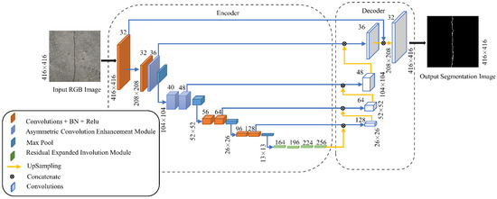
Figure 1.
Overall model framework of RIIAnet.
2.1. Involution Operator and Optimization Measures
2.1.1. Feature Extraction Method Based on Involution
Pavement cracks often have long and narrow shapes and diverse branches, but the small-sized convolution kernels commonly used in mainstream networks have difficulty in capturing the global features at one time, which limits the acquisition of context information by the convolution layer and reduces the accuracy of segmentation by the algorithm. To improve the accuracy of network identification of cracks, this paper introduces the involution [41] operator, which reduces the redundant information and strengthens the spatial modeling by sharing the weights of the channel dimensions. The channel information is then cleverly decoupled from the spatial information by the REI module, which was designed to achieve higher performance with fewer parameters.
Involution is an operator built on ordinary convolution that has the opposite properties of regular two-dimensional convolution. Based on the research of Li Duo et al. [41], in the spatial dimension, the same convolution kernel weights are shared on the same feature map called spatial invariance; in the channel dimension, each column of channels enjoys different groups of convolution weights called channel specificity. Convolution has properties such as being spatially agnostic and channel specific, while involution has the opposite properties because of the different methods of feature extraction.
The involution kernel is denoted as , where H denotes the length of the input feature map, W denotes its width, K denotes the size of the involution kernel, and G denotes the number of groupings. All channels share the G-group convolution kernel. The steps in the involution operation are as follows:
- The dimensions of the input feature maps are changed by averaging pooling.
- The channel dimensions are changed to by two convolution layers of size 1 × 1 with weight W.
- A grid of size K is used to spread the input feature maps and divide them into G groups.
- The obtained weights are multiplied and added to the spread feature maps. The feature mapping of each involution is obtained by multiplying and adding the values of the input features.
The mapping is defined as:
where denotes the involution kernel. The generic form of the involution kernel generation is as follows:
where is an index set of coordinate neighborhoods, and represents the feature maps of the slices after being passed through an unfolding operation. The function denotes the generated form of the weights W, and its expression is:
where and are the linear transformation matrices, denotes the channel reduction rate, and denotes the batch normalization and ReLU activation functions.
The involution operator is defined here with N = 1, G = 1, K = 2, and its features are extracted in the manner shown in Figure 2.
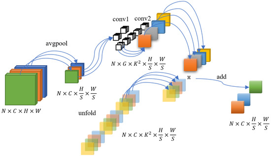
Figure 2.
Method of extracting feature maps in the involution operator.
To visually show the difference between the convolution and involution feature extraction methods, we put the analysis and visualization results of them in Section 3.3.
2.1.2. Optimization of the Involution Operator
We tried to use the bottleneck of Rednet-50 [41] to build and train the model, but we found that the loss function used for training converged with a normal trend when the model was trained without using the Rednet-50 pre-training weights, but the convergence of the loss function was harder in the validation set. We analyzed the reason for this result and improved the involution operator, the process of which is in Section 4.1.
Unlike the involution operator proposed by Li Duo et al. [41], the scheme in this paper, named involution-G, optimizes the involution operator by transforming the built-in batch normalization [42] into group normalization [43] with the number of groups setting to 16.
2.2. Residual Expanded Involution Module
To combine the advantages of both operators, we propose a new residual involution module that is different from the Rednet module in [41]. Based on the design criterion set out [40], we see that when the input dimensions are smaller than the output dimensions, the low-rank space cannot represent the high-rank space, causing the characteristic bottleneck problem. The authors of [40,44] showed that the hard-swish activation function has features including smooth and non-monotonic; its nonlinear nature means that it retains more information. It has also been experimentally shown that the hard-swish activation function can boost the rank of the data so that the rank of the input is closer to the rank of the output, thus reducing the representation loss.
Hence, the residual involution module in this paper adopts an expanded residual structure to retain as much information as possible. The difference between the REI module designed in this paper and other mainstream residual structures is shown in Figure 3.
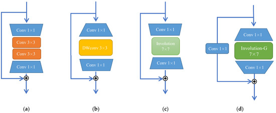
Figure 3.
Bottlenecks in (a) ResNet; (b) Mobilenet-v3; (c) Rednet-50 [41]; and (d) RIIAnet.
The REI module proposed in this paper involves dimensionally increasing convolution, dimensionally decreasing convolution, and involution. The operational steps are as follows:
- The feature map is expanded to the transition dimensions by convolution with a kernel size of 1 × 1 and a stride of one.
- Based on the experiments presented in [41], after weighting the performance and the number of parameters, we apply an involution kernel with a size of 7 × 7, the number of groups is set to 16, and a stride of one is used to perform feature extraction on the feature maps.
- The feature map extracted by involution is dimensionally reduced via conventional convolution with a kernel size of 1 × 1 and a stride of one.
- The input feature maps are dimensionally expanded through conventional convolution with a kernel size of 1 × 1 and a stride of one, and are added to the feature map extracted.
Here, we define as the number of input channels, as the number of transition channels, as the number of output channels, H and W as the length and width of the feature map, respectively. The details of the steps of the REI module are shown in Figure 4.
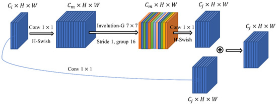
Figure 4.
Structure of the REI module.
The advantages of this structure are as follows:
- The extracted feature maps are dimensionally increased to enhance the nonlinear expression capability of the network, with a small increase in the computational effort.
- The involution operator is used to increase the perceptual field with fewer parameters to take advantage of the long-range dynamic modeling of involution and focus on the morphological information of the fracture.
- The dimensionality reduction process is used to decouple the spatial and cross-channel relationships of the feature maps [45] extracted by the involution module to achieve cross-channel information integration and enhance the feature expression capability of the network.
- We use the residual structure [46] to compensate for the loss of diversity information caused by the involution module, which makes the gradient flow propagate better and makes the network easier to train [47].
When building lightweight, real-time segmentation neural networks, the REI module is not suitable for use in shallow feature extractors, for which we give a detailed analysis in Section 4.2.
2.3. Asymmetric Convolution Enhancement Module
Conventional convolution does not meet our requirements for model accuracy. To further improve the ability of our network to extract cracks, based on the study in [45,48], we design an asymmetric convolution feature enhancement module as a way to obtain rich contextual information. This means that there are more effective features to be learned in the subsequent residual involution module, whose structure is shown in Figure 5.
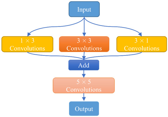
Figure 5.
Structure of the ACE module.
We intuitively display and analyze the extraction characteristics of asymmetric convolution and the ACE module for crack features. The results show that the ACE module can extract richer low-level features than the 3 × 3 convolution. The details are shown in Section 3.4.
2.4. Feature Fusion Module
Convolutional neural networks aim to extract different features of the input image, an approach that gives a different response at each layer of the feature extractor. The input image contains a richer level of detail in the shallow features while the focus in the deep features is on the semantic information of the image. The semantic information of pavement cracks is relatively straightforward, while the texture and edge information are complex and diverse. The construction of the network is crucial to retain the details of the crack information.
In this paper, we refer to the architecture of the U-Net [22] neural network and use a long connection structure to fuse the deep semantic information with the shallow edge information and to build the feature fusion module, whose structure is shown in Figure 6.
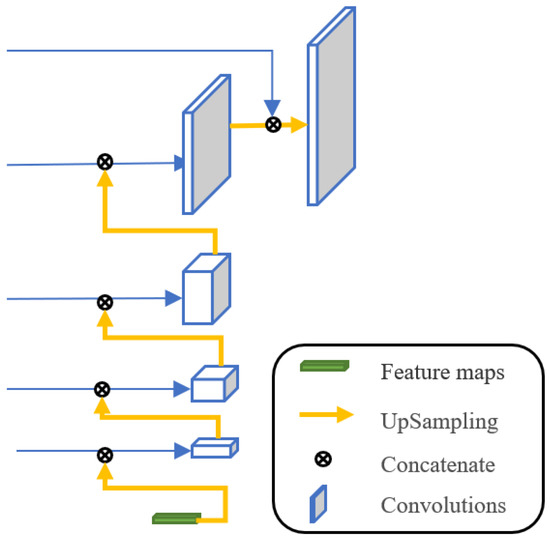
Figure 6.
Structure of the feature fusion module.
The deeper the network, the larger the field of view of the feature map and the better the grasp of the low-frequency information of the cracks. In contrast, a shallow network has better control of the local information and focuses on the extraction of the crack details. However, the level of detail is bound to be lost in the process of downsampling and feature extraction. The long connection structure is used to stitch the feature maps obtained from the encode part, which introduces high-frequency information with high resolution and also provides the spatial information required at the upsampling stage, making the segmentation mask more accurate.
3. Experiments and Results
In this section, we describe experiments carried out to verify the effectiveness and efficiency of the REI and ACE modules and the overall RIIAnet model designed in this paper. We first conducted experiments to analyze the roles of the above two modules in the network by varying the percentages of the different modules in the depth of the baseline network to select the appropriate positions of both in the network and ensure the network performance while maintaining inference speed. We then compare the performance of our RIIAnet network model with current advanced models to check the efficiency of our model. To comprehensively evaluate the performance of the module and the model, the metrics used in this paper are MIOU, MPA, Recall, F1 Score, and PR curve.
3.1. Datasets
The dataset in this paper consists of two parts. The first part was collected during a road survey in Zhengzhou using a 4-megapixel Hikvision industrial camera MV-CA060-10GC over different time periods under natural lighting conditions. The closer the camera to the road surface during collection, the smaller the field of view, the more accurate the overall information, and the clearer the crack texture. After numerous attempts, taking into account the overall layout and the branch details of the crack, it was determined that the optimum shooting distance was 60 cm from the road surface, and the shooting interval was set to 1 s. Finally, a total of 727 images were collected.
The second part of the dataset involves the Crack500 dataset, which was shot by Yang F. et al. [49] on the main campus of Temple University in the United States with a mobile phone. We used all the pictures from the Crack500 dataset.
Neural network training requires a large number of labeled datasets to prevent overfitting from occurring, so the data used in this article were generated through the following operations:
- Data preprocessing: if images that are too large are input into the deep convolutional network, there may be insufficient total graphics memory, resulting in training failure. In addition, the data we collected had a certain degree of randomness, which is not conducive to distinguishing between positive and negative samples during network training. Therefore, we resized the images in the original dataset to a resolution of 416 × 416 by compression and cropping, and selected 1278 images as our dataset through filtering. In addition, we screened the pavement materials with defects, where 496 images for asphalt, 236 images for concrete, 219 images for tar, and 277 images for gravel.
- Data augmentation: to meet the requirements of model training, we expanded the cropped dataset by rotating images through 90° and 180°, and applying horizontal and vertical flips and other image geometric transformations to give a final total of 5110 images. We randomly chose 3582 images as the training set, 765 as the validation set, and the remainder as the test set.
The heterogeneity of images affects the performance of crack detection [14,15]; as shown in Figure 7, to comprehensively test the robustness of the algorithm, the types of cracks included transverse, vertical, and network. Potholes, tire marks, shadows, and water stains were included as environmental disturbances in our datasets.

Figure 7.
(a) Vertical crack with wheel print; (b) horizontal cracks with shadow interference; (c) mesh cracks; (d) cracks with water stains; (e) cracks with potholes; and (f) cracks in asphalt and gravel mixtures pavement.
3.2. Experimental Environment and Parameter Settings
All experiments in this paper were implemented in Python, the deep learning framework was Pytorch 1.10.0 from the Artificial Intelligence Research Institute of Facebook company in the United States, and the operating system was Windows 10 developed by Microsoft in the United States. The hardware system included a main frequency Intel i9-9900k CPU, 32 GB of running memory, and an Nvidia GeForce GTX 2080 ti GPU with 11 GB of graphics memory.
The parameter settings of the model designed in this paper in the training process were as follows: the batch size was 16, Adam was used as the optimizer, the global initial learning rate was set to 1 × 10⁻³, the weight decay was set to 1 × 10⁻⁴, the loss function was BCELoss, and the learning rate method was CosineAnnealingLR. A total of 600 epochs was used to train the models, and their weights were saved every 20 epochs. The loss function curve of the model is shown in Figure 8.
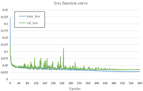
Figure 8.
Loss function curve of RIIAnet.
3.3. The Methods of Involution and Convolution for Crack Extraction
In Section 2.1.1, we described the feature extraction method of the involution operator. To further prove the opposite characteristics of involution and convolution, we visualized the extracted feature maps of them and analyzed their specialties. We used convolution and involution for feature extraction of the same input images and the results are shown in Figure 9 and Figure 10, respectively.
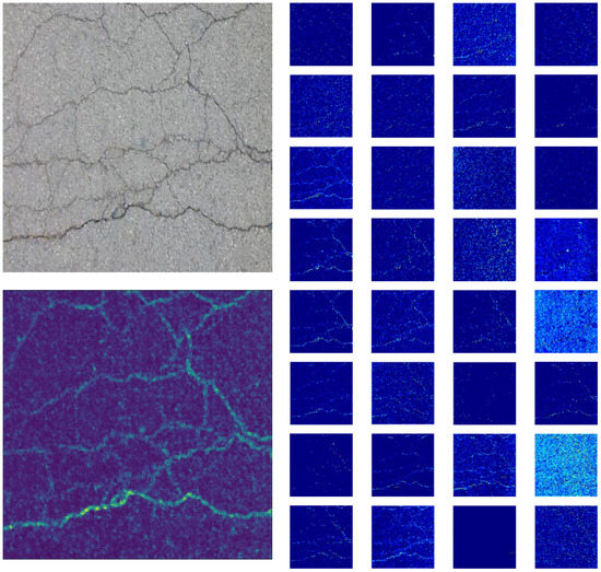
Figure 9.
Input image (top left), feature maps of the second stage in VGG-16, and fused image of feature maps (bottom left). The pictures are represented using 32 bits.
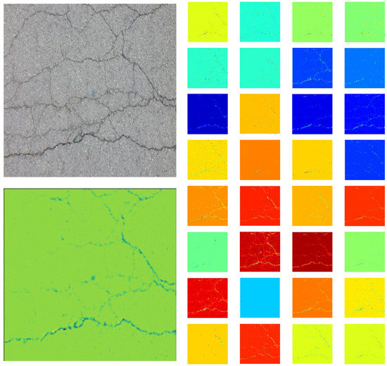
Figure 10.
Input image (top left), feature maps extracted by involution in the second stage in Rednet-50 [41], and fused image of feature maps (bottom left). The pictures are represented using 32 bits.
Due to the different weight parameters assigned by each convolution layer, the features extracted by each channel are also different from conventional convolution, as can be seen from Figure 9. Since existing mainstream networks use small convolution kernels for feature extraction, the correlation of the feature maps between channels is not close, and local field-of-view modeling is emphasized. Although feature extraction is relatively comprehensive, there are also numerous noise points in some feature maps. In addition, some studies [38,50] have shown that conventional convolution kernels have redundancy in the channel dimension and the performance on some feature maps is similar and even their reduction in the channel dimension will not affect the expressiveness.
When using involution for feature extraction, the feature maps of each channel containing certain crack features focus on the backbone information. This is because a single weight W is shared and generated for each group of feature maps. However, the unique channel invariance of involution limits the diversity of the crack features in the channel dimension and weakens the expression of the crack details, resulting in weaker extraction of the diversity of crack features via involution compared with conventional convolution.
3.4. Extraction Characteristics of Asymmetric Convolution and ACE Module for Cracks
Some existing studies [51,52,53] have shown that decomposing the standard n × n convolution into 1 × n and n × 1 convolutions for concatenation can reduce the number of parameters and the computation, but since in practice the kernels learned in deep networks have distributed feature values with an intrinsic rank higher than one, the direct application of 1 × n and n × 1 concatenation transformations can lead to significant information loss. Based on [48], we found that convolutional kernels with enhanced skeletons were more effective for feature representation. We used asymmetric convolution and convolution to extract the crack features, and the results are shown in Figure 11.
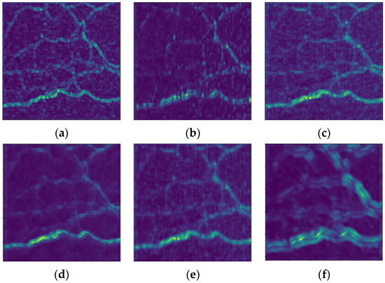
Figure 11.
(a) Input-fused image of feature maps; (b) fused image of feature maps after 1 × 3 convolutions extraction; (c) fused image of feature maps after 3 × 1 convolutions extraction; (d) fused image of feature maps after 3 × 3 convolutions extraction; (e) fused image of feature maps after parallelization of 1 × 3, 3 × 1, and 3 × 3 convolutions extraction; and (f) fused image of feature maps extracted by the ACE module. The above pictures are represented using 32 bits.
From Figure 11, we can see that the 1 × 3 convolution is more sensitive to horizontal cracks and the 3 × 1 convolution is more concerned with vertical cracks, while the 3 × 3 convolution plays more of a role in strengthening the backbone with better global feature extraction but a less good grasp of detail. Parallelization of the above three convolutions enhances the details of the cracks and the representation of the main features, but the feature representation is more saturated, and more noise is introduced compared to the 3 × 3 convolution. Hence, after parallelization, we use a 5 × 5 convolution kernel for expansion, which not only deepens the number of network layers but also performs inter-channel information interaction to reduce the noise and refine the crack features.
3.5. Performance Comparison of the REI Module with Different Occupancy Ratios
To determine the impact of the scaling relationship between regular convolution and the REI module on the performance of the model, we designed a 12-layer deep coding and decoding network in which the coding structure consisted of convolutions of size three with a step size of one, REI modules, and max-pooling. The decoder was consistent with the framework in Section 2.4. We used it as the baseline model.
We divided the baseline model according to the scale and configured it from deep to shallow layers. The proportion of the REI module to the baseline model was set to 0, 1/6, 1/3, 1/2, 2/3, 5/6, and 1. The relationship between the proportions of the convolution layer and the REI module in this network was determined by testing the inference speed and calculating the evaluation metrics. The training parameters were set as described in Section 3.2, and the training, validation, and test sets were the same as in Section 3.1. The results are shown in Table 1.

Table 1.
Comparison of experimental results for different ratios of REI modules in the baseline model.
To better evaluate the improvement in the network performance with the different module percentages, we used the PR curve to evaluate the impact on the model performance, and the result is shown in Figure 12.
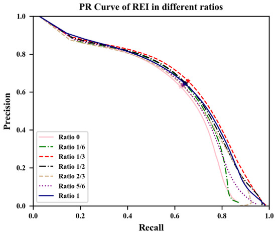
Figure 12.
Precision-recall curve for different ratios on the test set.
In summary, regardless of the comparison of performance indicators or using the PR curve to represent the performance of different proportions of convolution and REI modules, as the proportion of conventional convolutional layers increases, the speed of network inference is accelerated. This is due to the involution requiring more data reading-and-writing operations when performing inference compared to convolution, and the time lost to reading and writing is much larger than the time saved by the reduction in floating-point computations. Moreover, when involution is used for computation in shallow layers, the computational cost increases abruptly when large-resolution feature maps are unfolded, resulting in an obvious influence on the inference speed of the involution operator. In terms of the model capability, as the proportion of REI modules increases, the network performance increases first and then decreases. The model capability is optimal when the proportion is 1/3 and gradually decreases as the proportion becomes greater than 1/3. In view of this, we concluded that the attention patterns of distinct features are beneficial for the performance of the neural network at different levels. The shallow layers should be used to obtain as many features of the target as possible, while the deeper layers should reduce the channel redundancy, enhance the feature expression, and promote the classification capability of the network as a way to obtain higher model performance in terms of cost.
After balancing the inference speed and accuracy, from shallow to deep layers, we chose a configuration where regular convolution occupied 2/3 and the REI module occupied 1/3 of the overall network to build our encoder structure.
3.6. Ablation Study of ACE Module
In Section 3.4, we explained the characteristics of the different types of asymmetric convolution for crack extraction and proposed a solution to the feature saturation caused by parallelization of the asymmetric convolutions. To verify the effectiveness of our proposed asymmetric convolutional feature enhancement module, we designed ablation experiments using the same dataset as in Section 3.1, and the results are shown in Table 2.

Table 2.
Ablation study of the ACE module.
Compared with the model without the asymmetric feature enhancement module, the MIOU for the model with the feature enhancement module was improved by 0.0281, the MPA by 0.18%, the recall by 0.0443, and the F1 score by 0.0209. The inference speed was increased by 0.6 ms. This proves that although the asymmetric convolutional feature enhancement module increases the inference time to a certain extent, its asymmetric convolutional special perceptual field, which is exactly adapted to the narrow features of cracks, plays an important role in the shallow feature extraction network and can extract the information on the crack more comprehensively.
3.7. Performance Comparison of Different Models
3.7.1. Alternative Models
To verify the effectiveness of RIIAnet, we compared it with current state-of-the-art neural network segmentation models on the same dataset. The alternative models were BiseNet [34], Segnet [25], DeepLabv3+ [28], PSPnet [27], U-Net [22], UNet++ [24], and DeepCrack [26]. All algorithms were trained to converge in the same environment.
3.7.2. Comparison of Performance and Computation Metrics for Alternative Models
We measured the computational cost of the proposed model with the comparative models in Section 3.7.1 using floating-point operations (FLOPS) on an input image of size 416 × 416, using the number of parameters (Params) to represent the size of the model. The results are shown in Table 3.

Table 3.
Performance and computation metrics for different models.
It can be seen that RIIAnet has a certain advantage in terms of the parameters and floating-point operations while achieving high performance. The MIOU, MPA, recall, and F1 score of RIIAnet all reached the maximum of 0.7705, 0.9868, 0.8047, and 0.8485, respectively. Compared with the best U-Net network model in the alternative models, the improvements were 0.0062, 0.06%, 0.0117, and 0.0029, respectively and its size of parameters is 0.04 times that of U-Net and 0.03 times that of DeepLabV3+, while the floating-point operations are 1/33 of the former and 1/10 of the latter, respectively. Since RIIAnet was not designed with a complex decoder module to make it suitable for the device with low GPU computing resources, satisfactory results are achieved in the tradeoff between parameters and accuracy.
Figure 13 shows the PR curve, which is used to evaluate the generalization level and performance of the model from a qualitative perspective. It can be seen that the PR curve for RIIAnet on the test set completely exceeds those for the BiseNet, PSPnet, DeepLabV3+, and UNet++ models, indicating that its performance is better than these three models. This curve intersects with the Deepcrack, U-Net, and Segnet curves, and the performance of RIIAnet can be seen to be slightly higher than theirs based on the BEP performance metric (marked with an asterisk on the graph).
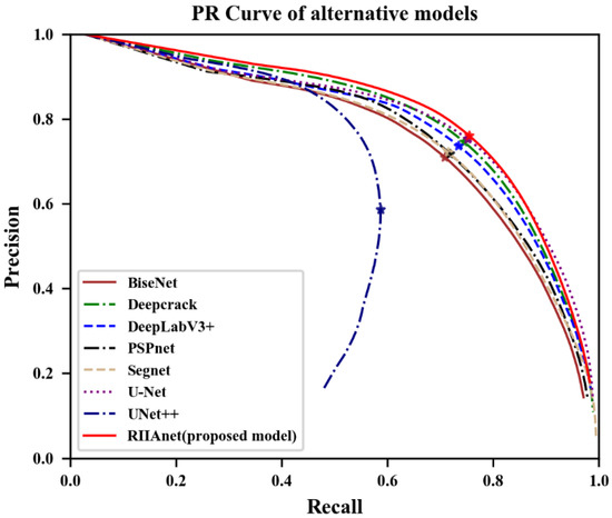
Figure 13.
Precision-recall curves for different models on the test set.
3.7.3. Comparison of the Inference Speeds of Alternative Models
When building a real-time segmentation model, the inference speed of the model is a crucial influencing factor. We compared the inference speed of the proposed network with the alternative models in Section 3.7.1, and the results are shown in Table 4.

Table 4.
Inference speeds for alternative models.
Since cracks are narrow, linear structures with a small percentage of pixels in the whole image, higher resolution means that more details of the cracks can be represented and higher accuracy of segmentation can be achieved, but the inference speed is reduced.
We tested the inference speed of the model at different resolutions of 416 × 416, 800 × 640, 1280 × 1024, and 2048 × 1024 in an inference environment based on an Nvidia Geforce RTX 2080 ti. In terms of speed, BiseNet was the fastest, followed by RIIAnet, meaning that both of these models can meet the demands of real-time segmentation under conditions of 2048 × 1024 high resolution; however, this is difficult for the U-Net, Deepcrack network models with good performance to achieve. Combined with the results of Section 3.7.2, in the trade-off between speed and accuracy, we think RIIAnet is more efficient.
3.7.4. Visualization of the Model Inference Results
Figure 14 illustrates the results of partial crack image prediction from the test set. To reflect the influence of image heterogeneity on different model detection, Figure 14 shows images, where the types of cracks are horizontal, vertical, and reticular; pavement materials include cement, asphalt, and concrete; environmental disturbances include shadows and wheel prints. As can be seen from column 1, compared with other segmentation networks, RIIAnet has a better global grasp and the shapes of the segmented cracks are more complete, which can be attributed to the advantages of long-range involution modeling. When the detected cracks are fine and complex (as shown in columns 2 and 3), BiseNet, DeeplabV3+, and PSPnet have higher missed detection rates, while Deepcrack, U-Net, and RIIAnet with fused encoding and decoding features have a significant effect. Under varying lighting and shading conditions (as shown in column 5), all eight algorithms extract cracks more completely, but with different levels of performance. RIIAnet shows better generalizability in predicting cracks in different pavement materials (as shown in column 6).
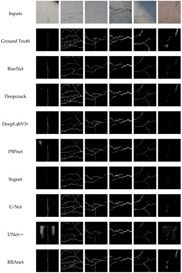
Figure 14.
Comparison of the results of different methods for six selected images from the test set.
3.7.5. Comparison of Crack Detection Performance under Different Pavement Materials
To verify the detection performance of our proposed algorithm in the heterogeneous images of different pavement materials, we use the test set of the Crack500 dataset after image processing to detect. The test set contains a total of 285 pictures, including 84 images for asphalt, 90 images for concrete, and 111 images for gravel. MIOU and inference speed are shown in Table 5.

Table 5.
Performance under different pavement materials.
The results show that RIIAnet has the best segmentation performance in asphalt and gravel materials, reaching the highest MIOU of 0.7222 and 0.7289, respectively; the MIOU of U-Net in concrete reaches the highest of 0.7252. In addition, the inference speed of RIIAnet is second only to BiseNet, with an average speed of 4.6 ms under images of 416 × 416 resolution. More importantly, compared with other models, RIIAnet shows excellent generalization, and its MIOU value fluctuates little under the pavement of different materials.
4. Discussion
4.1. Analysis of Involution Failing to Converge in the Validation Set
Since the performance was limited due to the hardware facilities available, the experiments in this paper did not include large batches of data operations at the same time, and the experiments on the Rednet-50 [41] network were conducted with batch sizes of 6 and 12. Loading the trained weights of the Rednet-50 model after 30,000 iterations revealed the presence of bad points in some of the images generated by the network, as shown in Figure 15.
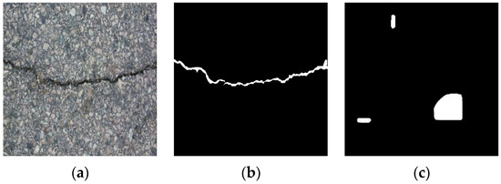
Figure 15.
(a) Input RGB image; (b) ground truth for the input image; and (c) dead segmentation image produced by Rednet-50.
Dead images such as this cause the loss functions for the validation set to fail to reach convergence. We found that the involution operator was more sensitive to the input data than conventional convolution, and the reasons for this are likely to be as follows:
- Batch normalization is calculated differently during training and validation. When small batches are used for training, the small-batch mean and variance are calculated each time and are used in the backpropagation of the gradient. However, in testing, the mean and variance precalculated for the training set via a sliding average are used for forwarding inference. When the distributions of the training and test data are significantly different, the precalculated mean and variance at training time do not effectively represent the distribution of test data that differ from the expected value.
- The involution operator performs parameter updating by quadratic optimization. When the distribution of the training data differs from the test data, the correlation between the weight W after batch normalization and the data obtained by spreading without normalization decreases. This results in the differences being continuously magnified, and bad points in the subsequent output of the deep network because of the decreasing resolution of the feature maps.
4.2. Analysis of the Efficiency of the REI Module
From the experimental results of Section 3.5, when building lightweight real-time segmentation networks, we believe the REI module does not play an obvious role in the shallow feature extraction module for the following reasons:
In terms of inference speed, we input the same data to the convolution and involution-G operators, respectively, to test their inference time. The experimental conditions include inputting the same data calculation amount, inputting the same size feature maps with a different number of channels, and inputting different size feature maps with the same number of channels. The results are shown in Figure 16, Figure 17 and Figure 18, respectively:
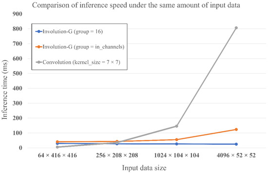
Figure 16.
Inference speed of convolution and involution-G operators under the same amount of data calculation.
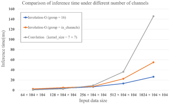
Figure 17.
Inference speed of convolution and involution-G operators under the same size feature maps with a different number of channels.
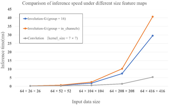
Figure 18.
Inference speed of convolution and involution-G operators under different size feature maps with the same number of channels.
We can find that the number of channels has a large impact on the inference speed of convolution, while the involution-G operator is more sensitive to the feature map size. The convolution weights are determined by fitting the data in the training phase, but the parameters in involution-G are dynamically calculated from the input data, which affects the inference speed of the involution-G operator when computing high-resolution feature maps. In addition, that involution-G requires more data reading-and-writing operations when performing inference compared to convolution. What is more, when involution-G is used for computation in shallow layers, the computational cost increases abruptly when large-resolution feature maps are unfolded, resulting in an obvious influence on the inference speed of the involution-G operator.
In terms of feature expression, as shown in Section 3.3, since involution focuses on modeling the spatial dimension and weakens the modeling relationship in the channel dimension, this affects the ability of involution to interact with information in the low channel dimension and has some influence on expressing the feature diversity in the shallow space.
The idea underlying convolution is to form global information from the combination of features in the local sensory field to make target judgments, and the computing power is allocated more to the channel dimension [54]. However, it was found in [39] that as the depth of the network increases, the relevance of the convolutional kernels becomes stronger, the diversification decreases, and the redundant information between channels becomes prominent. This means that the computing power is somewhat wasted in the deep network constructed by convolution; in contrast, involution can use larger convolutional kernels to increase the perceptual field without increasing the number of parameters, and use the sharing of weight parameters between channels to encode different semantic information to enhance spatial modeling and allocate more computing power to the spatial dimensions.
We combine the different characteristics of these two operators by employing convolution in the shallow network to integrate channel information and enrich the details of the crack feature by using the advantages of local pattern modeling in the high-resolution feature map; in the deep levels, we adopt the involution operator to take advantage of the large convolution kernel in the low-resolution feature map for long-range dynamic interaction modeling and exploit its unique spatial specificity to enhance the representation of the semantic information. This structure not only makes full use of the computing resources in the channel and spatial dimensions but also avoids the shortcomings of conventional convolution and involution in deep neural networks by amplifying each of them.
4.3. Analysis of ACE Module Effectiveness
The role of the proposed ACE module is to reduce the information loss of the crack features at the shallow feature extraction stage and to turn as many crack features as possible into abstract semantic information to pass to the involution operator in the deeper layer for semantic information enhancement. From the results of Section 3.4, it can be seen that the perceptual field of asymmetric convolution is different from that of convolution, and its special field of view matches the linear features of cracks, meaning that it can extract crack information from multiple aspects. However, due to the unique field-of-view mechanism of asymmetric convolution, some of the non-feature points are misjudged as points of interest for extraction, resulting in excessive noise after concatenation. To mitigate this effect, we promote the interaction and integration of information between channels by using large convolutional up-dimensioning to refine the crack features and attenuate the noise. From the results of Section 3.6, it can be seen that after adding the ACE module, the MIOU, MPA, recall, and F1 score of the model are improved by 0.0281, 0.18%, 0.0443, and 0.0209, respectively. This illustrates the effectiveness of the ACE module.
5. Conclusions
Pavement cracks are one of the early defects of roads that affect service life and driving safety. For practical engineering applications, pavement management departments need to check a large number of road miles. Huge model parameters and computational overhead are unaffordable or unnecessary. Considering that the DCNN models usually adopt a single-feature modeling method, a lightweight real-time segmentation network for pavement cracks is designed that adopts three methods of asymmetric convolution, convolution, and involution in different depths of the neural network. The core is to extract the low-level features of cracks in the shallow layers, and strengthen the expression of high-level features in the deep layers. The main work and conclusions of this study are as follows:
- To better reflect the real situation of road inspection, in Section 3.1, we construct the pavement defect dataset through field research and photography. Pavement materials include asphalt mixtures and cement concrete, and environmental disturbances were composed of shadows, water stains, and tire marks. This is beneficial to reflect the generalization performance and general applicability of the model.
- Convolution and involution have different extraction characteristics for crack features. In the shallow network, convolution is better for the detail extraction of cracks, focusing on channel-dimension modeling, while involution has a strengthening effect on the backbone information of cracks, focusing on spatial-dimension modeling.
- In Section 4.1, the experiment shows that the use of the involution under mini-batch training caused the validation set to not converge, and the output segmented binarized image had dead pixels. The built-in batch normalization of involution to group normalization, named involution-G, is changed to avoid the impact caused by differences in data distribution.
- To obtain the optimal position of the designed REI module, the results of the comparative experiments in Section 3.5 show that the effect is better when the REI module occupies 1/3 of the baseline model. Compared with the model using only convolution, MIOU, MPA, recall, and F1 score are improved by 0.0242, 0.92%, 0.0263, and 0.013, respectively. In Section 4.2, we analyzed the difference between involution-G and convolution from the perspectives of inference speed and feature construction, and explain why the REI module is effective in deep networks.
- The field of view of asymmetric convolution is more sensitive to cracks. Through the designed ACE module, the extraction of crack features in shallow networks is enhanced. In Section 3.6, the results show that by adding the ACE module, the MIOU for the model was improved by 0.0281, the MPA by 0.18%, the recall by 0.0443, and the F1 score by 0.0209.
- The proposed RIIAnet model is compared with semantic segmentation networks of different structures. The evaluation indicators and visualization results of Section 3.7 show that the MIOU, MPA, recall, and F1 score of RIIAnet reach 0.7705, 0.9868, 0.8047, and 0.8485, respectively. Its parameter amount is 0.04 times that of U-Net, and it can run in real time under high-resolution images.
In neural networks, the essence of network design is the mechanism used to allocate computing resources. For example, the attention mechanism in deep learning aims to emulate human vision [55], and the network performance can be improved by giving more attention to the target region at the particle level. Our proposed model improves the network performance by giving different attention patterns to different levels of the network at the macro level. The model proposed in this paper can reallocate limited computing resources in the spatial and channel feature modeling methods to achieve the effect of improving model performance with fewer parameters. Although the results show the performance improvement of the RIIAnet model for DCNN models with different architectures, further experiments are needed to pave the way for the real-time operation of low-power edge embedded devices.
Author Contributions
Conceptualization, P.Y. and N.W.; data curation, P.Y.; formal analysis, P.Y. and N.W.; methodology, P.Y. and N.W.; software, P.Y.; supervision, N.W.; validation, P.Y.; visualization, P.Y.; writing—original draft, P.Y.; writing—review and editing, N.W. All authors have read and agreed to the published version of the manuscript.
Funding
This work was supported by the National Training Program of Innovation and Entrepreneurship for Undergraduates (Grant No. 202110459036), the National Natural Science Foundation of China (Grant Nos. 51978630 and 52108289), Open Fund of Changjiang Investigation, Planning and Design Institute (Grant No. CX2020K10), and Key scientific research projects plan of colleges and universities in Henan Province (Grant No. 21A560013).
Institutional Review Board Statement
Not applicable.
Informed Consent Statement
Not applicable.
Data Availability Statement
The data presented in this study are available on request from the corresponding authors.
Conflicts of Interest
The authors declare no conflict of interest.
References
- CIA. Roadways—The World Factbook. Available online: www.cia.gov (accessed on 12 July 2021).
- CIA. Public Road Length—2017 Miles by Functional System. Available online: www.cia.gov/the-world-factbook (accessed on 2 February 2019).
- Abdellatif, M.; Peel, H.; Cohn, A.G.; Fuentes, R. Pavement Crack Detection from Hyperspectral Images Using a Novel Asphalt Crack Index. Remote Sens. 2020, 12, 3084. [Google Scholar] [CrossRef]
- Krysiński, L.; Sudyka, J. Gpr abilities in investigation of the pavement transversal cracks. J. Appl. Geophys. 2013, 97, 27–36. [Google Scholar] [CrossRef]
- Masserey, B.; Mazza, E. Ultrasonic sizing of short surface cracks. Ultrasonics 2007, 46, 195–204. [Google Scholar] [CrossRef] [PubMed]
- Glinicki, M.A.; Litorowicz, A. Crack system evaluation in concrete elements at mesoscale. Bull. Pol. Acad. Sci. Tech. Sci. 2006, 54, 371–379. [Google Scholar]
- Tang, Y.; Gu, Y. Automatic Crack Detection and Segmentation Using a Hybrid Algorithm for Road Distress Analysis. In Proceedings of the 2013 IEEE International Conference on Systems, Man, and Cybernetics, Manchester, UK, 13–16 October 2013; pp. 3026–3030. [Google Scholar] [CrossRef]
- Oliveira, H.; Correia, P.L. CrackIT—An image processing toolbox for crack detection and characterization. In Proceedings of the 2014 IEEE International Conference on Image Processing (ICIP), Paris, France, 27–30 October 2014; pp. 798–802. [Google Scholar] [CrossRef]
- Li, H.; Song, D.Y.; Liu, B.L. Automatic Pavement Crack Detection by Multi-Scale Image Fusion. IEEE Trans. Intell. Transp. Syst. 2019, 20, 2025–2036. [Google Scholar] [CrossRef]
- Zhao, H.; Qin, G.; Wang, X. Improvement of canny algorithm based on pavement edge detection. In Proceedings of the 2010 3rd International Congress on Image and Signal Processing, Yantai, China, 16–18 October 2010; pp. 964–967. [Google Scholar] [CrossRef]
- Shi, Y.; Cui, L.; Qi, Z.; Meng, F.; Chen, Z. Automatic Road Crack Detection Using Random Structured Forests. IEEE Trans. Intell. Transp. Syst. 2016, 17, 3434–3445. [Google Scholar] [CrossRef]
- Akiyoshi, H.; Takeshi, N. Development of a classification method for a crack on a pavement surface images using machine learning. In Proceedings of the SPIE 10338, Thirteenth International Conference on Quality Control by Artificial Vision 2017, Tokyo, Japan, 14 May 2017; Volume 103380M. [Google Scholar] [CrossRef]
- Hearst, M.A.; Dumais, S.T.; Osuna, E.; Platt, J.; Scholkopf, B. Support vector machines. IEEE Intell. Syst. Appl. 1998, 13, 18–28. [Google Scholar] [CrossRef] [Green Version]
- Pal, M.; Palevičius, P.; Landauskas, M.; Orinaitė, U.; Timofejeva, I.; Ragulskis, M. An Overview of Challenges Associated with Automatic Detection of Concrete Cracks in the Presence of Shadows. Appl. Sci. 2021, 11, 11396. [Google Scholar] [CrossRef]
- Palevičius, P.; Pal, M.; Landauskas, M.; Orinaitė, U.; Timofejeva, I.; Ragulskis, M. Automatic Detection of Cracks on Concrete Surfaces in the Presence of Shadows. Sensors 2022, 22, 3662. [Google Scholar] [CrossRef]
- Kim, J.J.; Kim, A.-R.; Lee, S.-W. Artificial Neural Network-Based Automated Crack Detection and Analysis for the Inspection of Concrete Structures. Appl. Sci. 2020, 10, 8105. [Google Scholar] [CrossRef]
- Jin, G.-S.; Oh, S.-J.; Lee, Y.-S.; Shin, S.-C. Extracting Weld Bead Shapes from Radiographic Testing Images with U-Net. Appl. Sci. 2021, 11, 12051. [Google Scholar] [CrossRef]
- Kim, B.; Cho, S. Automated Multiple Concrete Damage Detection Using Instance Segmentation Deep Learning Model. Appl. Sci. 2020, 10, 8008. [Google Scholar] [CrossRef]
- Shelhamer, E.; Long, J.; Darrell, T. Fully convolutional networks for semantic segmentation. IEEE Trans. Pattern Anal. Mach. Intell. 2017, 39, 640–651. [Google Scholar] [CrossRef] [PubMed]
- Yang, X.; Li, H.; Yu, Y.; Luo, X.; Huang, T.; Yang, X. Automatic Pixel-Level Crack Detection and Measurement Using Fully Convolutional Network. Comput. Aided Civil Infrastruct. Eng. 2018, 33, 1090–1109. [Google Scholar] [CrossRef]
- Ji, A.; Xue, X.; Wang, Y.; Luo, X.; Xue, W. An integrated approach to automatic pixel-level crack detection and quantification of asphalt pavement. Autom. Constr. 2020, 114, 103176. [Google Scholar] [CrossRef]
- Ronneberger, O.; Fischer, P.; Brox, T. U-Net: Convolutional Networks for Biomedical Image Segmentation. In Proceedings of the Medical Image Computing and Computer-Assisted Intervention—MICCAI 2015, Munich, Germany, 5–9 October 2015; MICCAI 2015. Lecture Notes in Computer Science. Navab, N., Hornegger, J., Wells, W., Frangi, A., Eds.; Springer: Cham, Switzerland, 2015; Volume 9351. [Google Scholar] [CrossRef] [Green Version]
- Liu, Z.; Cao, Y.; Wang, Y.; Wang, W. Computer vision-based concrete crack detection using U-net fully convolutional networks. Autom. Constr. 2019, 104, 129–139. [Google Scholar] [CrossRef]
- Zhou, Z.; Siddiquee, M.M.; Tajbakhsh, N.; Liang, J. UNet++: A Nested U-Net Architecture for Medical Image Segmentation. Deep Learning in Medical Image Analysis and Multimodal Learning for Clinical Decision Support. In Proceedings of the 4th International Workshop, DLMIA 2018, and 8th International Workshop, ML-CDS 2018, Held in Conjunction with MICCAI 2018, Granada, Spain, 20 September 2018; Volume 11045, pp. 3–11. [Google Scholar] [CrossRef]
- Badrinarayanan, V.; Kendall, A.; Cipolla, R. Segnet: A deep convolutional encoder-decoder architecture for image segmentation. IEEE Trans. Pattern Anal. Mach. Intell. 2017, 39, 2481–2495. [Google Scholar] [CrossRef]
- Zou, Q.; Zhang, Z.; Li, Q.; Qi, X.; Wang, Q.; Wang, S. DeepCrack: Learning Hierarchical Convolutional Features for Crack Detection. IEEE Trans. Image Process. 2018, 28, 1498–1512. [Google Scholar] [CrossRef]
- Zhao, H.; Shi, J.; Qi, X.; Wang, X.; Jia, J. Pyramid Scene Parsing Network. In Proceedings of the 2017 IEEE Conference on Computer Vision and Pattern Recognition (CVPR), Honolulu, HI, USA, 21–26 July 2017; pp. 6230–6239. [Google Scholar] [CrossRef]
- Chen, L.C.; Zhu, Y.; Papandreou, G.; Schroff, F.; Adam, H. Encoder-Decoder with Atrous Separable Convolution for Semantic Image Segmentation. In Proceedings of the Computer Vision—ECCV 2018, Munich, Germany, 8–14 September 2018; ECCV 2018; Lecture Notes in Computer Science. Ferrari, V., Hebert, M., Sminchisescu, C., Weiss, Y., Eds.; Springer: Cham, Switzerland, 2018; Volume 11211. [Google Scholar] [CrossRef] [Green Version]
- Chen, L.C.; Papandreou, G.; Kokkinos, I.; Murphy, K.; Yuille, A.L. Semantic image segmentation with deep convolutional nets and fully connected CRFS. Comput. Sci. 2014, 4, 357–361. [Google Scholar] [CrossRef]
- Chen, L.-C.; Papandreou, G.; Kokkinos, I.; Murphy, K.; Yuille, A.L. DeepLab: Semantic Image Segmentation with Deep Convolutional Nets, Atrous Convolution, and Fully Connected CRFs. IEEE Trans. Pattern Anal. Mach. Intell. 2018, 40, 834–848. [Google Scholar] [CrossRef] [Green Version]
- Chen, L.; Papandreou, G.; Schroff, F.; Adam, H. Rethinking Atrous Convolution for Semantic Image Segmentation. arXiv 2017, arXiv:abs/1706.05587. [Google Scholar]
- He, K.; Zhang, X.; Ren, S.; Sun, J. Spatial Pyramid Pooling in Deep Convolutional Networks for Visual Recognition. IEEE Trans. Pattern Anal. Mach. Intell. 2014, 37, 1904–1916. [Google Scholar] [CrossRef] [Green Version]
- Bai, R.; Jiang, S.; Sun, H.; Yang, Y.; Li, G. Deep Neural Network-Based Semantic Segmentation of Microvascular Decompression Images. Sensors 2021, 21, 1167. [Google Scholar] [CrossRef]
- Yu, C.; Wang, J.; Peng, C.; Gao, C.; Yu, G.; Sang, N. BiSeNet: Bilateral Segmentation Network for Real-Time Semantic Segmentation. In Computer Vision—ECCV 2018. ECCV 2018. Lecture Notes in Computer Science; Ferrari, V., Hebert, M., Sminchisescu, C., Weiss, Y., Eds.; Springer: Cham, Switzerland, 2018; Volume 11217. [Google Scholar] [CrossRef] [Green Version]
- Zhang, L.; Shen, J.; Zhu, B. A research on an improved Unet-based concrete crack detection algorithm. Struct. Health Monit. 2021, 20, 1864–1879. [Google Scholar] [CrossRef]
- Huang, G.; Liu, Z.; van der Maaten, L.; Weinberger, K.Q. Densely Connected Convolutional Networks. IEEE Comput. Soc. 2016, 4700–4708. [Google Scholar] [CrossRef]
- Zhang, Z.; Liu, Q.; Wang, Y. Road Extraction by Deep Residual U-Net. IEEE Geosci. Remote Sens. Lett. 2017, 99, 1–5. [Google Scholar] [CrossRef] [Green Version]
- Chen, Y.; Fan, H.; Xu, B.; Yan, Z.; Kalantidis, Y.; Rohrbach, M.; Shuicheng, Y.; Feng, J. Drop an Octave: Reducing Spatial Redundancy in Convolutional Neural Networks with Octave Convolution. In Proceedings of the 2019 IEEE/CVF International Conference on Computer Vision (ICCV), Seoul, Korea, 27 October–2 November 2019; pp. 3434–3443. [Google Scholar] [CrossRef] [Green Version]
- Zhang, Q.; Jiang, Z.; Lu, Q.; Han, J.; Zeng, Z.; Gao, S.; Men, A. Split to be slim: An overlooked redundancy in vanilla convolution. arXiv 2020, arXiv:2006.12085. [Google Scholar]
- Han, D.; Yun, S.; Heo, B.; Yoo, Y.J. Rethinking Channel Dimensions for Efficient Model Design. In Proceedings of the 2021 IEEE/CVF Conference on Computer Vision and Pattern Recognition (CVPR), New Orleans, LA, USA, 21–24 June 2021; pp. 732–741. [Google Scholar] [CrossRef]
- Li, D.; Hu, J.; Wang, C.; Li, X.; She, Q.; Zhu, L.; Zhang, T.; Chen, Q. Involution: Inverting the Inherence of Convolution for Visual Recognition. In Proceedings of the 2021 IEEE/CVF Conference on Computer Vision and Pattern Recognition (CVPR), New Orleans, LA, USA, 21–24 June 2021; pp. 12316–12325. [Google Scholar] [CrossRef]
- Ioffe, S.; Szegedy, C. Batch normalization: Accelerating deep network training by reducing internal covariate shift. CoRR 2015. [Google Scholar] [CrossRef]
- Wu, Y.; He, K. Group Normalization. Int. J. Comput. Vis. 2020, 128, 742–755. [Google Scholar] [CrossRef]
- Ramachandran, P.; Zoph, B.; Le, Q.V. Swish: A Self-Gated Activation Function. Arxiv Neural Evol. Comput. 2017. [Google Scholar] [CrossRef]
- Szegedy, C.; Vanhoucke, V.; Ioffe, S.; Shlens, J.; Wojna, Z. Rethinking the Inception Architecture for Computer Vision. In Proceedings of the IEEE Conference on Computer Vision and Pattern Recognition (CVPR), Las Vegas, NV, USA, 27–30 June 2016; pp. 2818–2826. [Google Scholar] [CrossRef] [Green Version]
- He, K.; Zhang, X.; Ren, S.; Sun, J. Deep residual learning for image recognition. In Proceedings of the 2016 IEEE Conference on Computer Vision and Pattern Recognition (CVPR), Las Vegas, NV, USA, 27–30 June 2016; pp. 770–778. [Google Scholar] [CrossRef] [Green Version]
- Hijazi, A.; Al-Dahidi, S.; Altarazi, S. A Novel Assisted Artificial Neural Network Modeling Approach for Improved Accuracy Using Small Datasets: Application in Residual Strength Evaluation of Panels with Multiple Site Damage Cracks. Appl. Sci. 2020, 10, 8255. [Google Scholar] [CrossRef]
- Ding, X.; Guo, Y.; Ding, G.; Han, J. ACNet: Strengthening the Kernel Skeletons for Powerful CNN via Asymmetric Convolution Blocks. In Proceedings of the 2019 IEEE/CVF International Conference on Computer Vision (ICCV), Seoul, Korea, 27 October–2 November 2019; pp. 1911–1920. [Google Scholar] [CrossRef] [Green Version]
- Yang, F.; Zhang, L.; Yu, S.; Prokhorov, D.; Mei, X.; Ling, H. Feature Pyramid and Hierarchical Boosting Network for Pavement Crack Detection. IEEE Trans. Intell. Transp. Syst. 2020, 21, 1525–1535. [Google Scholar] [CrossRef] [Green Version]
- Han, K.; Wang, Y.; Tian, Q.; Guo, J.; Xu, C. GhostNet: More Features from Cheap Operations. In Proceedings of the 2020 IEEE/CVF Conference on Computer Vision and Pattern Recognition (CVPR), Seattle, WA, USA, 13–19 June 2020. [Google Scholar] [CrossRef]
- Denton, E.L.; Zaremba, W.; Bruna, J.; LeCun, Y.; Fergus, R. Exploiting Linear Structure Within Convolutional Networks for Efficient Evaluation. NIPS 2014. [Google Scholar] [CrossRef]
- Jaderberg, M.; Vedaldi, A.; Zisserman, A. Speeding up convolutional neural networks with low rank expansions. Comput. Sci. 2014, 4, XIII. [Google Scholar] [CrossRef]
- Jin, J.; Dundar, A.; Culurciello, E. Flattened convolutional neural networks for feedforward acceleration. In Proceedings of the International Conference on Learning Representations (ICLR) 2015, San Diego, CA, USA, 7–9 May 2015. [Google Scholar] [CrossRef]
- Sun, Y.; Brockhauser, S.; Hegedűs, P. Comparing End-to-End Machine Learning Methods for Spectra Classification. Appl. Sci. 2021, 11, 11520. [Google Scholar] [CrossRef]
- Vaswani, A.; Shazeer, N.; Parmar, N.; Uszkoreit, J.; Jones, L.; Gomez, A.N.; Kaiser, Ł.; Polosukhin, I. Attention is all you need. arXiv 2017, arXiv:1706.03762. [Google Scholar]
Publisher’s Note: MDPI stays neutral with regard to jurisdictional claims in published maps and institutional affiliations. |
© 2022 by the authors. Licensee MDPI, Basel, Switzerland. This article is an open access article distributed under the terms and conditions of the Creative Commons Attribution (CC BY) license (https://creativecommons.org/licenses/by/4.0/).