Application of Particle Swarm Optimization for Improvement of Peel Strength in a Laminated Double-Lap Composite Joint

Abstract

A double lap joint is commonly used in thin structures under low running loads. Peel and inter-laminar stresses are among the major limitations of this type of joint, which may cause delamination failure. These stresses should be determined for designing a stronger structure. This study presents a method based on particle swarm optimization to find the best layup for a classic double lap joint under horizontal constant tensile forces. The peel stress equation is analytically obtained and utilized as the objective function for the algorithm. The method’s accuracy is explored by assessing the algorithm’s ability. This helps to find the best arrangement with the highest strength delamination against considering four initial layups. The results show that the optimized layups, on average, can reduce peel stress by about 96%. Additionally, the effects of different parameters on joint strength are investigated.

1. Introduction

Adhesive joints are increasingly used for joining composite structures or dissimilar materials in aerospace and automotive industries. Adhesive joints have unique advantages compared with traditional mechanical fasteners, which have to deal with the problems of loosening clamping force and fatigue strength, due to the spiral shape of the bolt-nut thread, wherein high-stress concentration factor occurs at the first bolt thread [1] and the load distribution in threads are uneven [2]. Composite materials have been increasingly used in aerospace, military, automobile, and other industries. Special characteristics of these materials, such as the significant strength–weight ratio, wear resistance, and thermal resistance, have further promoted their application scope, as they are substituting conventional materials.

Furthermore, the manufacturing process of composite materials is changing. For example, the 3D printing of curvilinear fiber-reinforced composite structures (CFRCS) is a novel approach in this area with fast development [3]. Various methods have been utilized to connect composite parts, among which the single lap joint, double lap joint, and steep single lap joint are the most well-known methods. Therefore, defining its connections is one of the most important aspects of designing a composite structure [4]. According to the statistics, almost 70% of the failures in structures occur in their joints [5]. These challenges make this area more interesting for researchers from different points of view. Yang and Pang presented an analytical solution for a composite single-lap joint based on the mechanics of composites and anisotropic laminated plate theory [6]. The method was developed to define the location and magnitude of the peel and shear stress distributions in the adherents and adhesive. Additionally, an FEA code was used to validate the proposed methodology results.

Tsai and Morton [7] compared the analytical and numerical results of single lap joints under tensile force. At first, the classical Goland and Reissner method was reversed and modified in an analytical solution. Then the results were compared with a 2D finite element model. Stress analysis for a composite adhesively bonded lap joint was proposed by Her [5]. Then the analytical results of a single lap joint and a double lap joint were compared with their corresponding FEM results. Zhang et al. [8] considered 3D stress analysis in composite joints. They developed and combined equations presented by Mortensen [9] via Hypersizer to derive a new way to calculate inter-laminar stress. The resulting equations were numerically solved and compared with the FE model. This method is applicable to a wide range of adhesive joints.

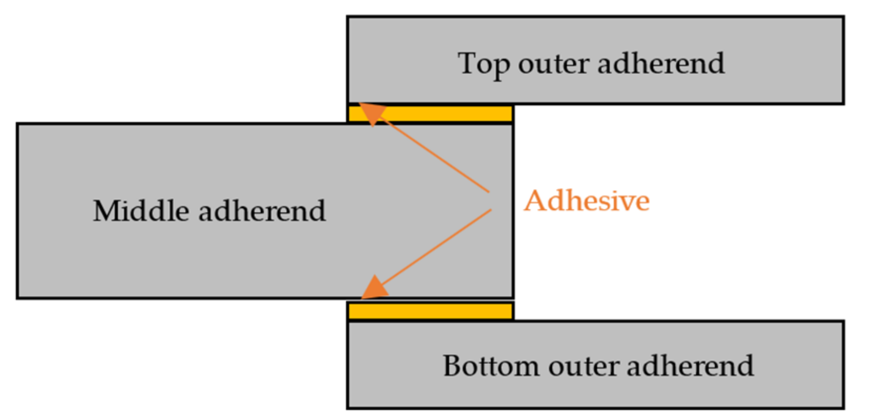
Classic composite joints are made of two or three adhesive adherends bonded together. The adherends in these joints can be the same (fiber-reinforced polymer (FRP) to FRP) or dissimilar (FRP to steel). A classic double lap joint consists of three adherends bonded two by two with adhesive layers, shown in Figure 1. The thickness of the middle adherend can be the same as the outer ones.

Joint modeling was carried out assuming geometrical symmetry based on the Reissner–Mindlin stacking plates theory. Finally, the results were validated relative to a finite element solution. Tsai and Morton [10] experimentally, numerically, and analytically investigated and compared the stress of the composite double lap joints. The stress of a bonded–bolted Al-GFRP double lap joint was experimentally and numerically explored by Di Franco and Zuccarello [11]. Their results were compared with an adhesively bonded joint and a bolted joint. The strength of the hybrid joint was higher than both simple joints against fatigue, energy absorption, and static tensile loads. An analytical solution was proposed by Arjomandi et al. to calculate peel stress in a double-lap joint under tensile force using classic laminate theory [12]. A finite element model in ANSYS validated the accuracy of the equation. Saleh et al. [13] conducted an experimental, analytical and numerical survey on stress analysis and damages of a double-lap steel-to-CFRP joint. The data containing FEM, digital image correlation (DIC), and acoustic emission (AE) were compared, and their convergence was illustrated.

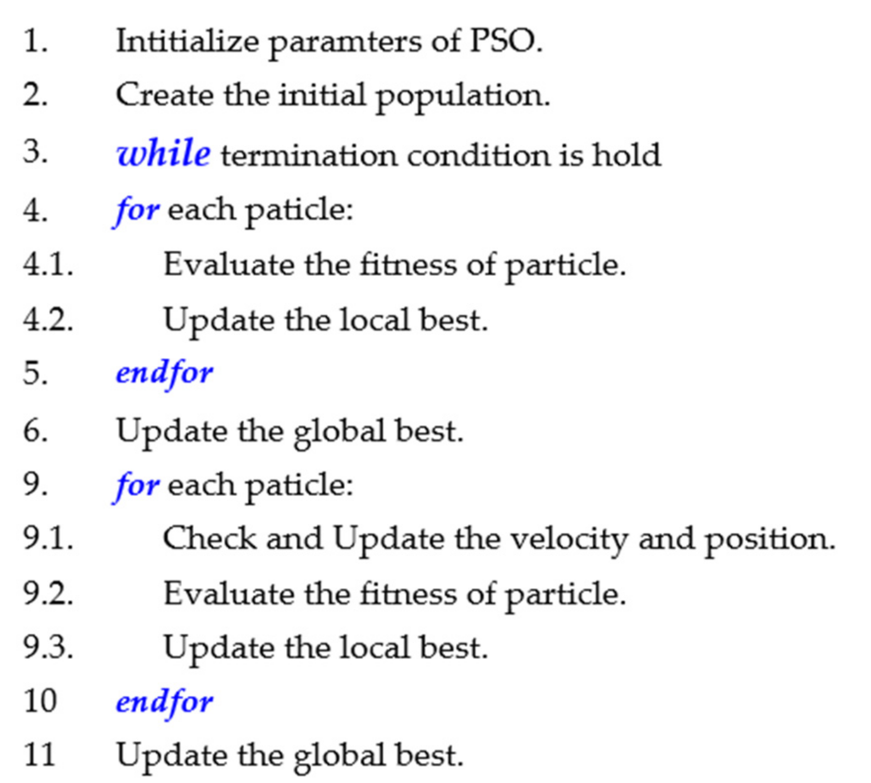
On the other hand, the application of optimization algorithms in complex problems has increased in recent decades. Kennedy and Eberhart [14] introduced the particle swarm optimization methodology for optimizing nonlinear functions. They investigated the relations of the novel method with GA and artificial life. They introduced a novel algorithm that simulates how a flock of birds behaves in their social community. So, they called this new search method particle swarm optimization (PSO).

Its initial purpose was to simulate the unforeseeable and distinguished choreography of a flock of birds graphically, to discover the patterns governing the ability of birds to fly synchronously and suddenly change direction by regrouping in an optimal formation. This simple concept was developed and led to an uncomplicated and effective optimization method.

In this methodology, the particles can fly and search through a hyperdimensional space. The basis of changes in the position of particles is the social–psychological propensity of them to imitate the prosperity of others. So, these changes for every individual are affected by the knowledge and experiences of other particles in their neighborhood. Therefore, it influences individual fashions in searching the area that the others do in the swarm (so, the PSO is a symbiotic collaborative algorithm, in other words). Utilizing this type of social manner as an optimization method results in the particles returning to the prior successful areas of exploration territory stochastically.

Basic particle swarm optimization formulas are

$$v_{ij}\left(t+1\right)=\omega \times v_{ij}\left(t\right)+c_1\times r_{1j}\left(t\right)\times \left[y_{ij}\left(t\right)-x_{ij}\left(t\right)\right]+c_2\times r_{2j}\left(t\right)\times \left[{\widehat{y}}_j\left(t\right)-x_{ij}\left(t\right)\right]$$

(1)

$$x_{ij}\left(t+1\right)=x_{ij}\left(t\right)+v_{ij}\left(t+1\right)$$

(2)

where $v_{ij}$ is the velocity vector and $x_{ij}$ shows the position of the particle. $c_1$ and $c_2$ are two constant values between 1.4 and 1.7. $r_{1j}\left(t\right)$ and $r_{2j}\left(t\right)$ are two random values ranging from 0 to 1. In the velocity equation,

$$\mathrm{Momentum} \mathrm{part}: \omega \times v_{ij}\left(t\right)$$

(3)

$$\mathrm{Cognitive} \mathrm{part}: c_1\times r_{1j}\left(t\right)\times \left[y_{ij}\left(t\right)-x_{ij}\left(t\right)\right]$$

(4)

$$\mathrm{Social} \mathrm{part}: c_2\times r_{2j}\left(t\right)\times \left[{\widehat{y}}_j\left(t\right)-x_{ij}\left(t\right)\right]$$

(5)

This optimization method has two subsidiaries: global best PSO (gbest PSO) and local best PSO (lbest PSO). For the global best PSO, the neighborhood for each particle is the entire swarm, while the local best PSO utilizes a social network cluster topology with smaller vicinities for every particle. This paper uses the lbest methodology to find the optimum layups. In local best PSO, the social part indicates information interchanged within the vicinity of the particle, illustrating the local understanding of the territory. Concerning the velocity equation, the social subsidy to particle velocity corresponds to the distance between a particle, and the best position found in the vicinity of particles. The velocity can be thus calculated as

$$v_{ij}\left(t+1\right)=\omega \times v_{ij}\left(t\right)+c1\times r_{1j}\left(t\right)\times \left[y_{ij}\left(t\right)-x_{ij}\left(t\right)\right]+c2\times r_{2j}\left(t\right)\times \left[{\widehat{y}}_j\left(t\right)-x_{ij}\left(t\right)\right]$$

(6)

where $y_{ij}\left(t\right)$ is the best position ever visited by the particle, $x_{ij}\left(t\right)$ is the particle’s current position and ${\widehat{y}}_j\left(t\right)$ shows the local best-visited position in the neighborhood. The pseudo-code of PSO is shown in Appendix B (Figure A1).

Imran et al. [15] explored the different modifications of the PSO methodology. The ability of these methods to find the optimum point of the objective function takes too much attention from specialists in different areas. In addition, they can be used as a significant substitution for costly and time-consuming experimental optimization methods. A combined algorithm was proposed by Kaveh et al. [16] to design composite plates subjected to in-plane loadings with minimum thickness. The model mixed charged system search (CSS) with PSO and used fiber orientation and the number of plies as the algorithm’s variables. Bavi et al. [17] proposed a combined BA-GA optimization method to ratchet the specific strength and capacity of single-lap and double-lap mixed adhesive joints. The algorithm was focused on geometry and manufacturing restrictions to find the optimal joint design. Rodriguez et al. proposed an evolutionary structural optimization (ESO) model for optimizing single-lap and double-lap joints [18]. The focus of the ESO model is on reducing peak stresses by shaping the adherends contour under a von Mises rejection criterion.

Arhore et al. [19] surveyed the effects of joint characteristics on its strength. They used a genetic algorithm and topology optimization to optimize the joint’s geometry. According to the results, the type of load was important in the effectiveness of the geometry. Topology optimization (TOP) presented a greater strength geometry; overall, GA suggested a better strength-to-weight ratio solution. Lu et al. [20] used machine learning to introduce a model, a multi-objective gray wolf optimizer combined with a support vector machine, for predicting the properties of composite materials. The model used six datasets to infer properties from available data. The model’s accuracy ranged from 0.14% to 5.574%, depending on the quality of input data.

Hassan Vand et al. [4] proposed an optimization method based on the bees algorithm (BA) for reducing the peel and shear stresses in a single lap joint under bending moment by rearranging the layup of its adherends. A finite element model was used to verify the analytically derived stress equations. Raut et al. [21] proposed a method based on structural health monitoring (SHM) to detect and classify the damages in the composite structures due to low-velocity impact (LVI). The study revealed that it improved the computational time of conventional methods by optimizing their computational techniques by utilizing optimization algorithms, such as GA, PSO, and neural networks.

Smith and Norato [22] proposed a novel method for maximizing the stiffness of composite structures made of fiber-reinforced cylindrical bars at a constant amount of material. The method is based on topology optimization and validated by numerical examples. Huang et al. [23] implemented fish swarm and frog leaping optimization methods to detect the damages of carbon fiber reinforced plastic π adhesive-bonded joints. Chen et al. [24] introduced a combined PSO-FEM model to optimize the design of composite laminates to have minimum peel stress. Yusoff et al. [25] used a particle swarm optimization algorithm to predict the behavior of single and double timber composite joints subjected to tensile force.

One of the common fractures in adhesive joints is over-allowed peel stress in the adhesive area. Previous studies investigated the various methods to calculate peel stress magnitude in adhesive-bonded joints, but the lack of a tool for optimizing the offered arrangement of adherend layers for reducing peel stress was obvious. So, the main purpose of this paper is to introduce an intelligence optimization method instead of expensive experimental ones for finding the best ply stacking sequence that leads to the highest peel strength in the adherends of a double lap joint using the analytically derived peel stress Equation [12] as the objective function of the particle swarm optimization algorithm. This algorithm was selected due to its feasibility and convergence. Adherend layers were assumed to be orthotropic, and the joint was symmetric and under tensile force. Additionally, the effect of joint geometric characteristics on this stress was investigated.

The organization of the remaining section of this study is as follows. A detailed explanation of modeling and governing stress equations are conducted and reported in Section 2. The effect of joint geometry on peel stress is reviewed and explored in Section 3. Section 4 provides the implementation of the optimization approach for double lap joint layup. In Section 5, results and discussions are elaborated. Lastly, Section 6 embodies the conclusion.

2. Modeling and Governing Stress Equations

The analytical solution for obtaining governing peel and shear stresses equations in adhesively bonded lap joints was investigated previously by Mortensen [9] and Zhang et al. [8], and differential equations were obtained and used in numerical methods to find the amount of stresses. However, PSO needs an objective function to find the optimum value, so the analytical solution was extended by Arjomandi et al. [12] to find a formula for calculating peel stress in a 2D double lap joint. In addition, a similar survey was conducted by Her and Chun [26] to extract an equation for calculating peel stress in a double lap joint.

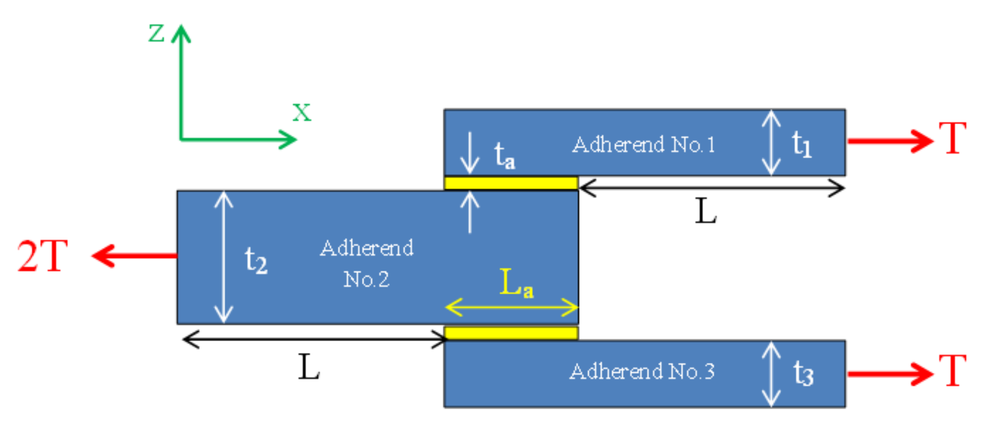
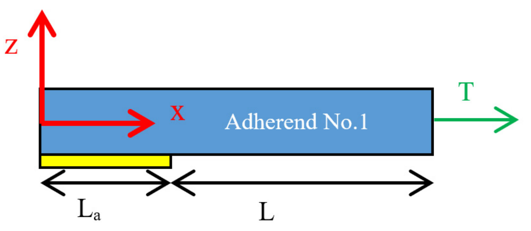
Therefore, here, a brief survey and their validation are presented, where the paper’s main purpose is to introduce a tool based on PSO to design the adherends to have the minimum peel stress. Adherends Nos. 1 to 3 are laminated layers bounded by adhesive layers (Figure 2). The thickness of adherends Nos. 1 and 3 (t₁ and t₃) is the same, and adherend No. 2 has a double thickness (t₂). The thickness of the upper and lower adhesive layers (t_a) is equal.

La and L in Figure 2 are the adhesive-area length and out-of-adhesive-area length, respectively.

Assumptions are as follows:

• Strains of each layer are in plane.
• Adherend layers are orthotropic.
• Adhesive layers are elastic.
• Since the joint is only under a tensile force (N_x = T) and layers are assumed to be wide and thin, the dependency of stress and strain to the y-axis ($\frac{\partial }{\partial y}$) is neglected, and just the relationships with the x-axis are considered.
• Classic plate theory (CPT) is used to extract governing equations.
• Based on CPT, shear force (Q) can be defined as

  $$Q={{\displaystyle \int }}_{\raisebox{1ex}{$-t$}\!\left/ \!\raisebox{-1ex}{$2$}\right.}^{\raisebox{1ex}{$t$}\!\left/ \!\raisebox{-1ex}{$2$}\right.}\tau dz$$

  (7)

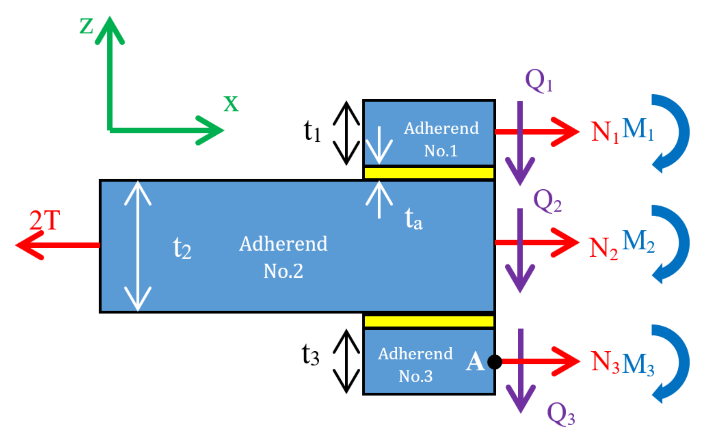
Each adherend’s free body diagram (FBD) was used to obtain equilibrium equations. Here, free body diagram of upper adherend (adherend No.1) is illustrated in Figure 3.

$${\tau }_1=-\frac{d{N}_1}{dx}$$

(8)

$${\sigma }_1=\frac{d{Q}_1}{dx}$$

(9)

$$\frac{d{M}_1}{dx}=Q_1+{\tau }_1\left(\frac{t_1}{2}+\frac{t_a}{2}\right)$$

(10)

The equilibrium equations for adherends Nos. 2 and 3 can be obtained similarly. Due to the elasticity assumption for adhesive layers, Hooke’s law is governing, so normal and shear stresses for the upper adhesive layer will be

$${\tau }_1=\frac{G_a}{t_a}\left(u_{01}+\left(\frac{t_1}{2}\right)\frac{d{w}_1}{dx}-u_{02}+\left(\frac{t_2}{2}\right)\frac{d{w}_2}{dx}\right)$$

(11)

$${\sigma }_1=\frac{E_a}{t_a}\left(w_2-w_1\right)$$

(12)

where $u_{01}$, $u_{02}$, $w_1$ and w₂ are the mid-surface displacements of adherends Nos. 1 and 2 in the x and z directions. In addition, E_a and G_a denote Young’s and shear moduli of adhesive, respectively. The stress equations for the lower adhesive layer (No. 3) can be similarly obtained.

Now, the equations for calculating displacements should be extracted. For this purpose, substitute the applied forces and moments into the stiffness matrix for the orthotropic adherend materials.

$$\left[\begin{array}{c}N\\ M\end{array}\right]=\left[\begin{array}{cc}A& B\\ B& D\end{array}\right]\left[\begin{array}{c}\epsilon \\ k\end{array}\right]$$

(13)

where k is the curvature in the x-direction.

Finally, Equations (14) and (15) illustrate the relationship between displacement, forces, and moments of the three adherends.

$$\frac{d{u}_{0i}}{dx}=\frac{B_{11}^i}{{\left(B_{11}^i\right)}^2-D_{11}^i{A}_{11}^i}{M}_i+\frac{D_{11}^i}{{\left(B_{11}^i\right)}^2-A_{11}^i{D}_{11}^i}{N}_i$$

(14)

$$\frac{d^2{w}_i}{d{x}^2}=\frac{A_{11}^i}{{\left(B_{11}^i\right)}^2-A_{11}^i{D}_{11}^i}{M}_i+\frac{D_{11}^i}{{\left(B_{11}^1\right)}^2-A_{11}^i{D}_{11}^i}{N}_i$$

(15)

In these equations, the upper indices of $A_{11}^i$, $B_{11}^i$ and $D_{11}^i$ (elements of A, B, and D matrices) depict the number of the adherends (i = 1–3). On the other hand, according to FBD (Figure 4), there are relationships between forces and moments (around point A) of three adherends, as shown in Equations (16) and (17).

$$N_2=2T-N_1-N_3$$

(16)

$$M_2=2T\left(\frac{t_2}{2}+t_a+\frac{t_3}{2}\right)-M_1-M_3-N_1\left(\frac{t_1}{2}+t_2+2t_a+\frac{t_3}{2}\right)-N_2\left(\frac{t_2}{2}+t_a+\frac{t_3}{2}\right)$$

(17)

Combining Equations (14) and (15) with the first derivative of Equation (11) and substituting Equations (16) and (17) into the resulting expression while using the first derivative of Equation (2), we have

$$\frac{d^2{N}_1}{d{x}^2}=-\frac{G_a}{t_a}\left(k_1{M}_1+k_2{N}_1+k_3{M}_3+k_4{N}_3+k_{5}T\right)$$

(18)

Additionally, by implementing Equations (15)–(17) in the first derivative of Equation (12),

$$\frac{d^2{\sigma }_1}{d{x}^2}=\frac{E_a}{t_a}\left(k_6{M}_1+k_7{N}_1+k_8{M}_3+k_9{N}_3+k_{10}T\right)$$

(19)

where ki (i = 1–10) are constraints of thicknesses of the joint and stiffness matrix arrays as expressed in Appendix A. In the same way, it is possible to find similar equations for $N_2$ and ${\sigma }_2$. Equation (20) is formed by derivation and a combination of Equations (8)–(10).

$$\frac{d^4{M}_1}{d{x}^4}=\frac{d^2{\sigma }_1}{d{x}^2}-\frac{d^4{N}_1}{d{x}^4}\left(\frac{t_a+t_1}{2}\right)$$

(20)

Now, substitute Equation (19) into Equation (20).

$$\frac{d^4{M}_1}{d{x}^4}=k_6{M}_1+k_7{N}_1+k_8{M}_3+k_9{N}_3+k_{10}T-\frac{d^4{N}_1}{d{x}^4}\left(\frac{t_a+t_1}{2}\right)$$

(21)

Due to the symmetry of the joint, these relationships are correct: $N_1=N_3$ and $M_1=M_3$. To substitute them in equations obtained for forces and moments and also in Equations (16) and (17), the differential equation of changes according to x is as follows:

$$\frac{d^6{N}_{x1}}{d{x}^6}+{\delta }_1\frac{d^4{N}_{x1}}{d{x}^4}+{\delta }_2\frac{d^2{N}_{x1}}{d{x}^2}+{\delta }_3{N}_{x1}={\delta }_{4}T$$

(22)

where coefficients ${\delta }_i\left(i=1-4\right)$ are calculated via equations of $k_i$ as mentioned in Appendix A. So, the changes in horizontal force $N_1$ are calculable by solving differential Equation (22):

$$N_1\left(x\right)=c_{1}ex{p}^{q_{1}x}+c_{2}ex{p}^{-q_{1}x}+c_{3}ex{p}^{x\sqrt{q_2+q_{3}i}}+c_{4}ex{p}^{x\sqrt{q_2-q_{3}i}}+c_{5}ex{p}^{-x\sqrt{q_2+q_{3}i}}+c_{6}ex{p}^{-x\sqrt{q_2-q_{3}i}}+\frac{T{\delta }_4}{{\delta }_3}$$

(23)

where c_i (i = 1–6) are differential equation coefficients that boundary conditions can obtain. Additionally, $q_i$ (i = 1–3) are parameters related to ${\delta }_i$ that are expressed in Appendix A. Now, it is possible to find the peel stress equation from Equation (23) that expresses the force variations along the x-axis. At first, it is necessary to find the trend of bending moment changes along the x-axis. So the M₁ equation is formed from the symmetry assumption, and Equation (21) is as follows:

$$\begin{gathered} M_1\left(x\right)={\theta }_1{c}_{1}ex{p}^{q_{1}x}+{\theta }_1{c}_{2}ex{p}^{-q_{1}x}+{\theta }_2{c}_{3}ex{p}^{x\sqrt{q_2+q_{3}i}}+{\theta }_3{c}_{4}ex{p}^{x\sqrt{q_2-q_{3}i}}+{\theta }_2{c}_{5}ex{p}^{-x\sqrt{q_2+q_{3}i}} \\ +{\theta }_3{c}_{6}ex{p}^{-x\sqrt{q_2-q_{3}i}}-\frac{T{k}_5}{k_1+k_3} \end{gathered}$$

(24)

where ${\theta }_i$ (i = 1–3) are calculated via equations explained in Appendix A. Additionally, according to Equation (8),

$$\begin{gathered} {\tau }_1\left(x\right)=-q_1{c}_{1}ex{p}^{q_{1}x}+q_1{c}_{2}ex{p}^{-q_{1}x}-\sqrt{q_2+q_{3}I}{c}_{3}ex{p}^{x\sqrt{q_2+q_{3}I}}-\sqrt{q_2+q_{3}I}{c}_{4}ex{p}^{x\sqrt{q_2-q_{3}I}}+ \\ \sqrt{q_2+q_{3}I}{c}_{5}ex{p}^{-x\sqrt{q_2+q_{3}I}}+\sqrt{q_2-q_{3}I}{c}_{6}ex{p}^{-x\sqrt{q_2-q_{3}I}} \end{gathered}$$

(25)

Based on the third relation obtained from FBD of adherend No. 1, the changes of $Q_{\mathrm{i}}$ can be expressed in the following equation.

$$N_1\left(x\right)=c_{1}ex{p}^{q_{1}x}+c_{2}ex{p}^{-q_{1}x}+c_{3}ex{p}^{x\sqrt{q_2+q_{3}i}}+c_{4}ex{p}^{x\sqrt{q_2-q_{3}i}}+c_{5}ex{p}^{-x\sqrt{q_2+q_{3}i}}+c_{6}ex{p}^{-x\sqrt{q_2-q_{3}i}}+\frac{T{\delta }_4}{{\delta }_3}$$

(26)

Appendix A expresses the coefficients of ωi (i = 1–6) in the above equation. Now, the formulas defined for $N_1$, $M_1$, and $Q_1$ and governing boundary conditions can be employed for adherend 1 to specify differential equation constants. Assume that the coordinates origin is located on one left end of adherend 1 (Figure 5), so the boundary conditions are

$$@ x=0 : N_1=M_1=Q_1=0$$

(27)

$$@ x=L_a+L : N_1=T \& M_1=Q_1=0$$

(28)

The differential equation coefficients are calculated by substituting these boundary conditions into Equations (23), (24) and (26). Therefore, the peel stress equation can be determined by

$$\begin{array}{l}{\sigma }_1\left(x\right)={\omega }_1{q}_1{c}_{1}ex{p}^{q_{1}x}-{\omega }_2{q}_1{c}_{2}ex{p}^{-q_{1}x}+{\omega }_3\sqrt{q_2+q_{3}i}{c}_{3}ex{p}^{x\sqrt{q_2+q_{3}i}}+{\omega }_4\sqrt{q_2-q_{3}i}{c}_{4}ex{p}^{x\sqrt{q_2-q_{3}i}}\\ -{\omega }_5\sqrt{q_2+q_{3}i}{c}_{5}ex{p}^{-x\sqrt{q_2+q_{3}i}}-{\omega }_6\sqrt{q_2-q_{3}i}{c}_{6}ex{p}^{-x\sqrt{q_2-q_{3}i}}\end{array}$$

(29)

A finite element model in ANSYS was used to validate the analytical solution and find the maximum peel stress location and magnitude in the adhesive layer [12]. It was assumed that the adherends are Graphite–Epoxy T5208/300 and adhesive layers are Metbond 408. The mechanical properties of these materials are mentioned in

Table 1. Mechanical properties of selected materials.

Material Name	ν	G (GPa)	Ez (GPa)	Ex (GPa)
Graphite-Epoxy	0.280	7.170	10.300	181
Metbond	0.343	0.358	-	0.96

.

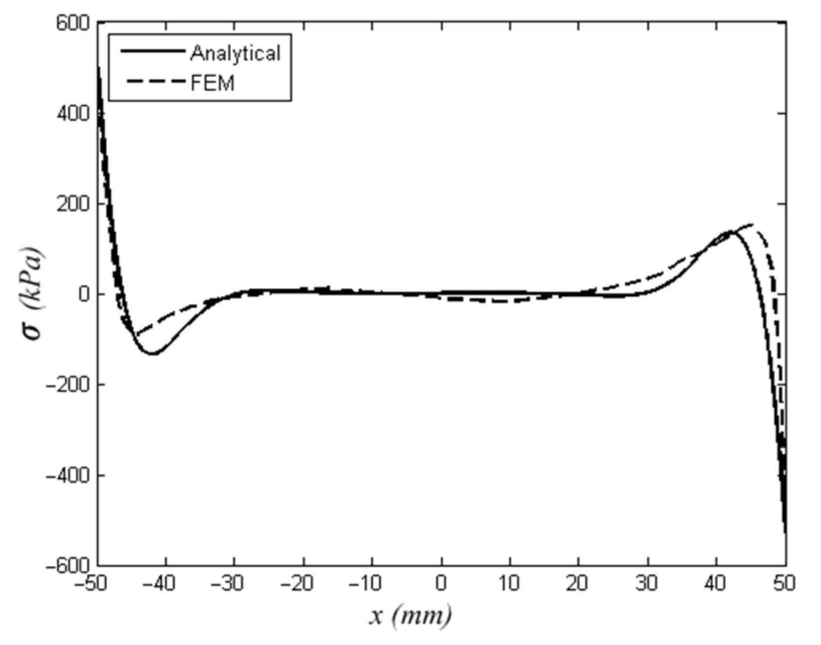
Accordingly, the maximum peel stress occurred at both ends of the adhesive area, and the analytical solution results are perfectly acceptable, compared to the finite element model results [12]. The differences between analytical and FEM solutions of peel stress along the adhesive area are shown in Figure 6. The maximum peel stress calculated via analytical solution is 473.08 kPa, where the FEM gives a 501.65 kPa output in the same conditions. The differences between those two methods are 6.04 percent.

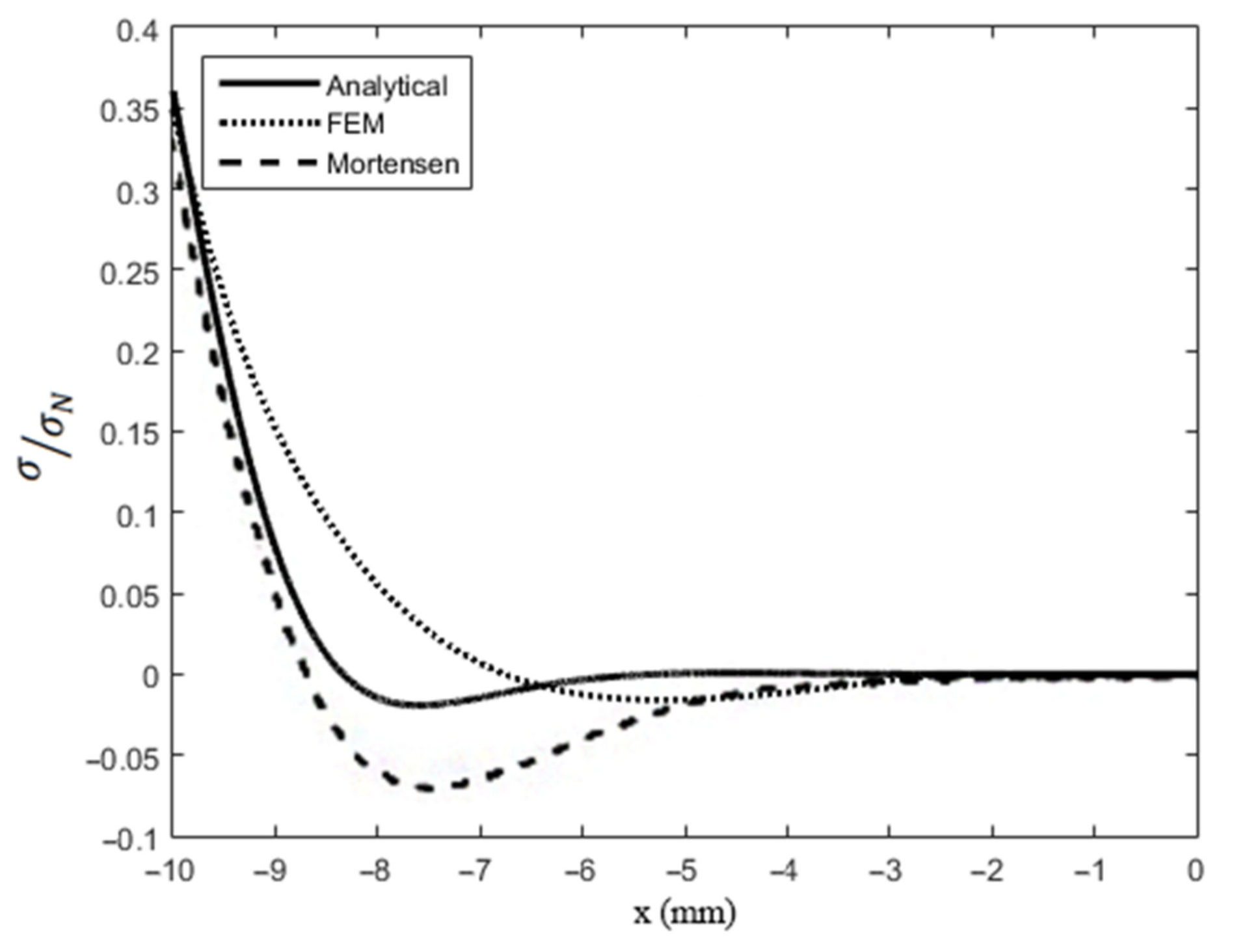
The horizontal axis in Figure 6 is the length of the adhesive area, and the vertical axis illustrates the peel stress magnitude. As mentioned before, the highest peel stress amplitude occurs at both ends of the adhesive area. The differences between the outcomes of the analytical solution (Equation (29)), FEM, and the result obtained by Mortensen [9] for a classic double lap joint are illustrated in Figure 7. According to the graphs, the dimensionless maximum peel stress obtained from the analytical solution is 0.36, whereas the FEM and Mortensen methods reported it as 0.35 and 0.33, respectively. Therefore, the analytical model which is used in this paper is more accordant with the FEM.

3. Effect of Joint Geometry on Peel Stress

The layer arrangement of adherend No 1 is mentioned in this section since adherends 1 and 3 are the same and adherend 2 has a layer arrangement like that of adherend 1, but double the number of layers. In this section, we investigated the effect of each geometrical characteristic on peel stress by changing the parameters of Equation (29). In each subsection, just one of the parameters is variable, and the others remain constant. Joint dimensions in the next analyses are as follows: the adherend’s initial arrangement is [0₁₂], adhesive length is 100 mm, the thickness of each lamina is 0.3 mm, adhesive layers thickness is 0.3 mm, and the length of adherends out of the adhesive area is 100 mm. The applied force is 100 N/m. Adherends are Graphite–Epoxy T5208/300, and the adhesive is Metbond 408.

3.1. Effect of Fiber Angle on the Peel Stress

This section keeps all previous joint geometry specifications constant, and the only variant is fiber angle. The angle of fibers in adherends 1 and 2 was changed, and its effect on the peel stress was investigated as listed in

Table 2. Variation in maximum peel stress due to changes in fiber angle.

Arrangement of Adherend No. 1	Maximum Peel Stress Magnitude (KPa)
[012]	73.566
[±156]	111.11
[±306]	425.03
[±456]	5.9467 × 103
[±606]	5.755 × 105
[±756]	2.8548 × 108
[±906]	8.4404 × 109

. As shown, peel stress amplitude was increased with an enhancement in the fibers’ angle. Overall, the joint strength will decrease at a specific loading by increasing the fiber angle. The percentage of increase in the peel stress at each step ascends approximately linearly. The variation of peel stress relative to a joint with zero fibers angle is shown in Figure 8.

As expected, the adherend with zero angle fibers has the most strength since the fibers are aligned with the applied tensile force. The strength of the joint is reduced by increment in fibers’ angle, and obviously, the adherend with [±90₆] arrangement is the weakest because the fibers are perpendicular to the force.

3.2. Effect of Number of Adherend Plies on the Peel Stress

All the joint parameters are kept constant while the number of plies is varied.

Table 3. Variation in maximum peel stress due to changes in the number of layers.

Arrangement of Adherend No. 1	Maximum Peel Stress Magnitude (KPa)
[05]	1188.9
[010]	121.35
[015]	41.731
[020]	21.390

lists the influence of the number of piles on the peel stress.

According to Table 3, maximum peel stress falls by increasing the number of layers. Obviously, the strength of the joint is improved with a rise in the number of plies with fibers aligned to a constant force since more layers will endure the stress. The change rate is not linear and reduced on a larger number of layers.

Table 4. Variation in maximum peel stress by increasing the number of layers.

Arrangement of Adherend No. 1	Percentage of Changes in the Number of Layers	Percentage of Changes in Peel Stress	Peel Stress Changes According to Adding Each Layer
[010]	100%	−89.79%	−17.96%
[015]	50%	−65.61%	−13.12%
[020]	33%	−48.74%	−9.75%
[025]	25%	−38.1%	−7.62%
[030]	20%	−31.12%	−6.22%

illustrates the percentage of stress changes with adding more layers, and these changes are calculated relative to the previous arrangement. The data which are presented in the first row are compared with peel stress related to the [0₅] arrangement.

According to the data mentioned in Table 4, the improvement rate of the strength of the joint will rise slightly in larger layers.

3.3. Effect of the Thickness of the Adhesive Layer

In this section, all the geometric characteristics are kept constant but thickness. The results are presented in

Table 5. Variation in maximum peel stress due to a change in thickness of the adhesive layer.

The Thickness of the Adhesive Layer (mm)	Maximum Peel Stress Magnitude (KPa)
0.1	10,915
0.2	382.38
0.3	73.566
0.5	11.252
0.7	3.3922

.

As observed, an increase in the thickness of the adhesive layer declines the maximum peel stress, while the joint strength is increased. This reverse relationship comes from constant factor equations explained in Appendix A. It means that the thicker adhesive layer has more strength against deformation. The trend of these changes is reduced at large thicknesses.

Table 6. Variation in maximum peel stress by changing the thickness of the adhesive layer.

Rate of Thickness Change (mm)	Percentage of Thickness Change	Percentage of Changes in Peel Stress
0.1	100%	−96.5%
0.1	50%	−80.76%
0.2	66%	−84.7%
0.2	40%	−69.85%

illustrates the trend of changes in peel stress by increasing the adhesive thickness. The rate of changes in thickness is related to the thicknesses mentioned in Table 5. The results show that even fewer changes in the rising thickness of the adhesive layer can cause a significant impact on peel stress.

3.4. Effect of the Thickness of the Adherend

In this section, the laminae thickness was increased step by step. The peel stress magnitude was calculated as presented in

Table 7. Variation in maximum peel stress changes in each lamina’s thickness.

The Thickness of Lamina (mm)	Maximum Peel Stress (kPa)
0.1	2882.5
0.15	611.13
0.2	235.83
0.25	121.35

. By enhancing the thickness of adherends, the stress decreased, while the joint strength experienced growth. A thicker adherend can show a better behavior against deformation, and according to the coefficients of Equation (29), which are expressed in Appendix A, an increase in laminae thickness will decrease the peel stress magnitude.

4. Double Lap Joint Layup Optimization

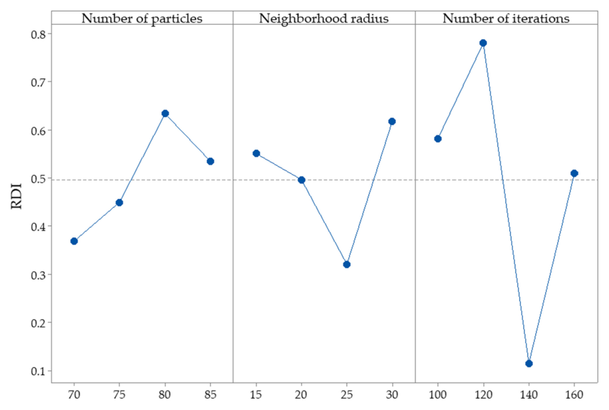
The particle swarm optimization method was used to optimize the stress equation. To tune the parameters of PSO and find the optimum level of parameters, we use design of experiment (DOE) techniques, among which the Taguchi method is one of the most applicable DOE methods for optimization purposes. For more information, refer to [27,28]. We design the Taguchi orthogonal array L₁₆ based on

Table 8. Local particle swarm optimization algorithm settings.

Parameters	Level of Parameters	Optimum Level
Number of particles	70, 75, 80, 85	70
Neighborhood radius	10, 15, 20, 25	25
Number of iterations	100, 120, 140, 160	140

and calculate the objective function for adherend No. 1 as [±45/0/±15]s, [±30/±60/902/02]s, [±75/0/±15/0/±15]s, and [±75/±60/±45/±30/±15/02]s, 30 times. Then, we calculate the relative deviation index (RDI) [27] to convert the results to the same scales. Afterward, the Taguchi method is created for “Smaller is Better”. The result of the Taguchi method is shown in Figure 9 and Table 8.

The results were examined for different numbers of particles, various neighborhood radii, and different iterations. Finally, the settings mentioned in Table 8 were chosen in terms of the accuracy and computational cost of the optimization process. The maximum peel stress was evaluated in each iteration, and for each layer arrangement, with a change in the sort of layers in the next iteration, the stress was re-calculated. The arrangement with minimum peel stress is presented. MATLAB software was used to solve the equations and programming. Convergence diagrams of optimized joints are presented in Figure 7, Figure 8, Figure 9 and Figure 10. The geometric features of the joints are the same as what was mentioned at the beginning of Section 3.

Equation (29) was introduced to the program as the objective function. Four different joints were considered to find out how much the optimization could effectively reduce the peel stress in balanced and unbalanced joints.

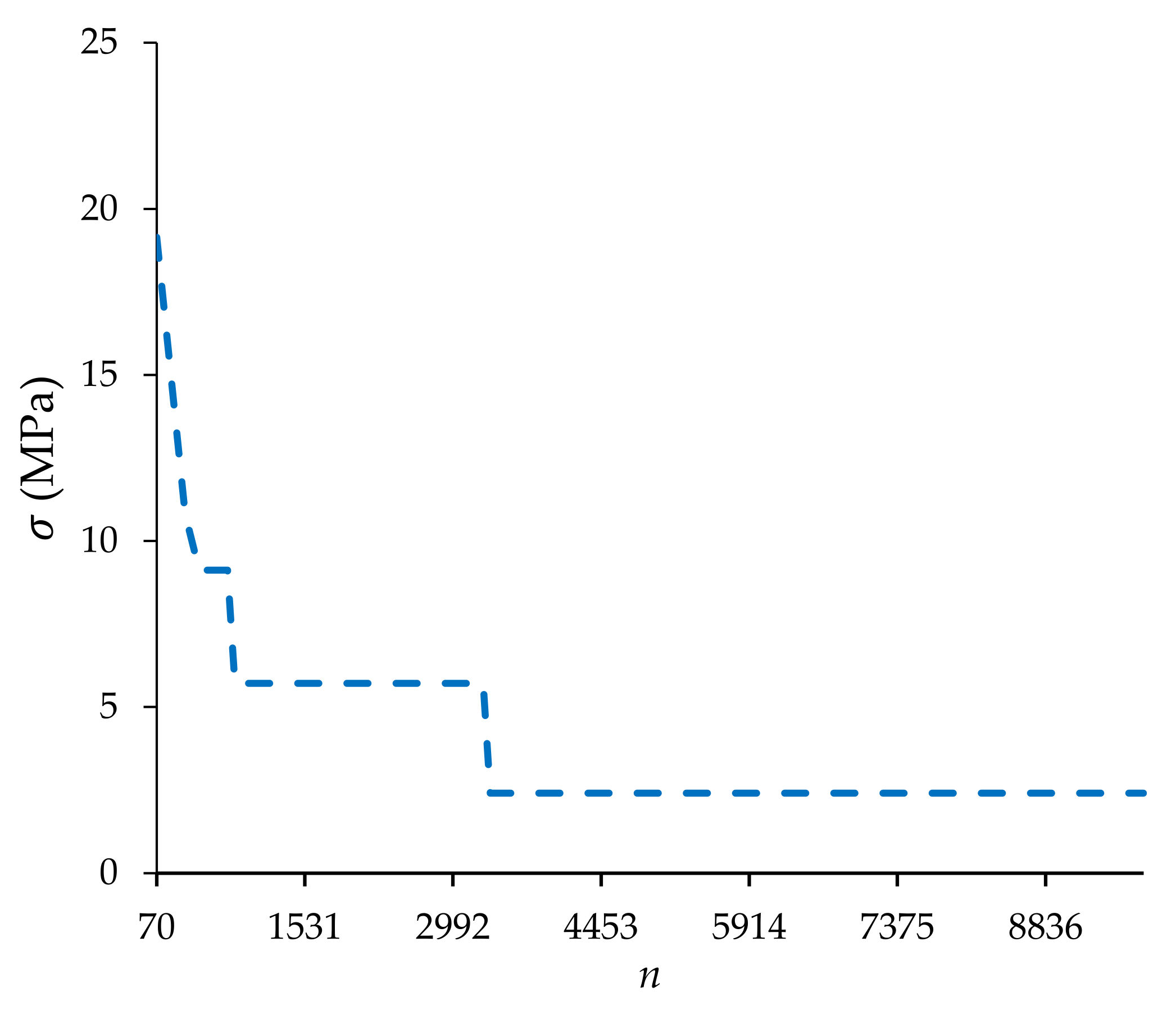
Case number 1:

For [±45/0/±15] s initial arrangement of adherend No. 1, the best layer arrangement was [±15/±45/0] s. The maximum peel stress was 30.35 MPa for the initial design, which declined to 2.406 MPa after optimization, causing a 92% decrement. The convergence diagram of the optimization algorithm is depicted in Figure 10. As it is shown, the algorithm can reach the answer after 3360 iterations.

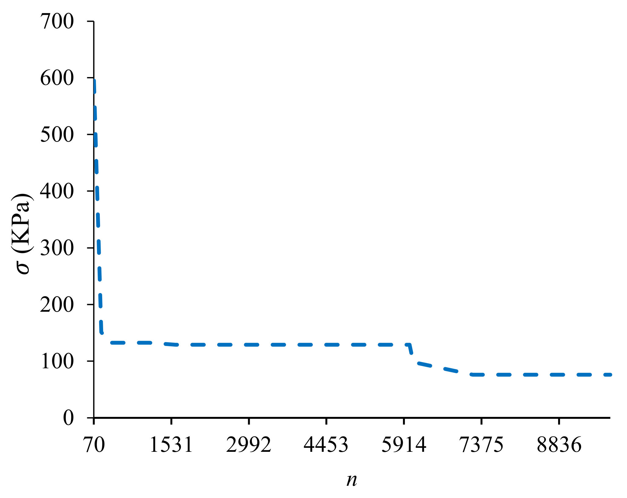
Case number 2:

For the initial arrangement of adherend No. 1 as [±30/±60/902/02] s, the best layer arrangement was [902/±60/±30/02] s. The maximum peel stress was 1.77 MPa for the initial design, which was reduced (by 95.7%) to 75.95 kPa after optimization. The convergence diagram is shown in Figure 11. The vertical axis shows the magnitude of max peel stress in each iteration, and the horizontal axis shows the number of calculating objective functions (stress equation). As it is shown, the algorithm can reach the answer after 7210 iterations.

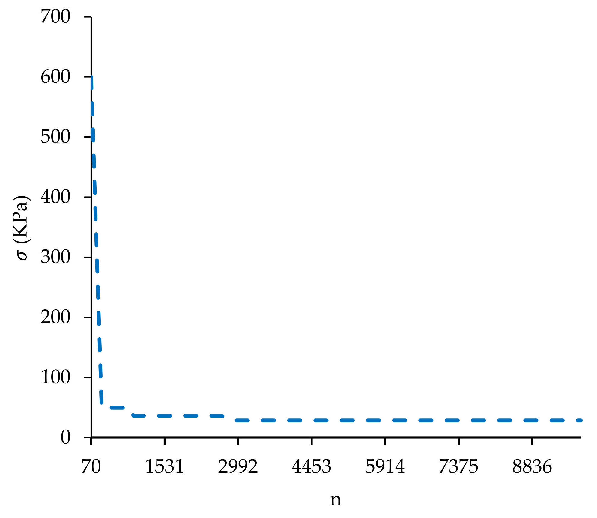
Case number 3:

Considering the initial arrangement of [±75/0/±15/0/±15] s for adherend No. 1, the best layer arrangement was [0/±152/±75] s. The maximum peel stress of the initial design was 1.2 MPa, which showed a 97.6% decrement and reached 28.4 kPa after optimization. The convergence diagram of the optimization algorithm is presented in Figure 12. As seen, the algorithm can reach the answer after 2660 iterations.

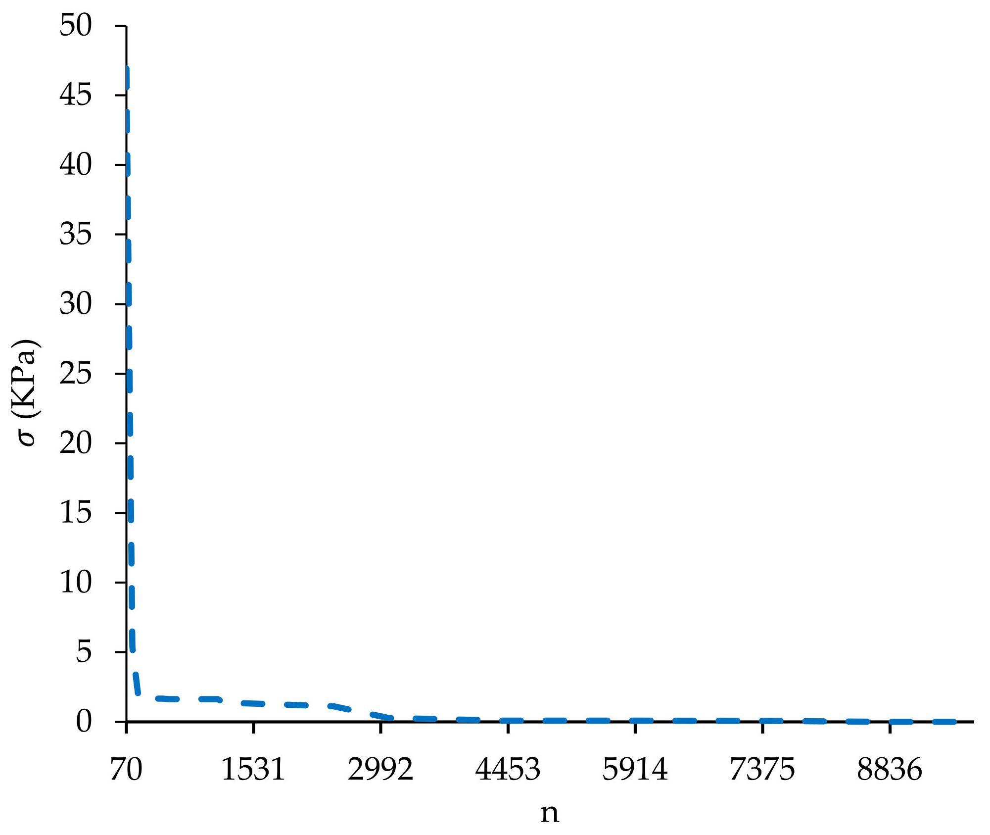
Case number 4:

For the initial arrangement of adherend No. 1 as [±75/±60/±45/±30/±15/02] s, the best layer arrangement was [0/±60/±75/±30/0/±15/±45] s. The maximum peel stress was 99.55 kPa for the initial design, which was reduced to 0.0065 MPa after optimization, showing a 99% decline. The convergence is depicted in Figure 13. As shown, the algorithm can reach the answer after 8820 iterations.

5. Results and Discussion

Peel stress magnitude increased at larger fiber angles, reducing the joint strength under loaded tensions. Therefore, the best choice for a joint under horizontal tensile force is to adherends with zero angle fibers (i.e., along force direction). At a specific load and fiber angle, peel stress magnitude is decremented by increasing the number of layers due to a rise in the stiffness of matrix arrays. Additionally, the maximum peel stress is connected to the number of layers. The adherends with more layers have more strength against the same tensile force. This is because of the improvement of the stiffness matrix arrays. The adhesive layer thickness undeniably affects the magnitude of peel stress at both sides of the joints and adhesive–adherend interface. This is because of the better strength of a thicker adhesive against deformation. The rate of variations is significant in smaller thicknesses, causing the growth of the peel stress. Therefore, it is possible to boost the mechanical properties of the joint by increasing the thickness of the adhesive layer. An increment in the thickness of adherends increases the stiffness matrix arrays. This could significantly reduce peel stress and improve joint characteristics. Based on the results, the most effective peel stress geometrical characteristics are the fiber angle, the adhesive layer thickness, the thickness of adherends, and the number of adherends, respectively.

Regarding the convergence diagrams in the last section, the local particle swarm optimization method shows a magnificent capability to find the best arrangement leading to the minimum peel stress accurately and quickly. As mentioned in the optimization of the layer arrangement, mounting layers with different fiber angles can affect the joint strength against peel stress. This method can be a tool for designers and researchers who want to investigate the geometrical parameters’ effects and optimize the ply stacking sequence of a double lap joint without executing expensive experimental tests.

6. Conclusions

In the design of adhesive-bonded composite joints, one of the major concerns is failure due to high peel stress at the edge of the bonding area. So, it is essential to take care of every geometrical factor impact on the maximum peel stress. Therefore, this paper presents the effects of some joint characteristics on peel stress and introduces a method based on particle swarm optimization to find the best ply stacking sequence for an offered layer arrangement that causes minimum peel stress. According to the results, the most effective parameter on the magnitude of peel stress is the angle of fibers in a double lap joint. For a constant tensile force, perpendicular fibers produce a peel stress magnitude 114 million times greater than that of aligned fibers. The number of plies in each adherend is another parameter that is investigated. The changes in maximum peel stress are not linear, and where doubling the layers from [0₅] to [0₁₀] can reduce it by approximately 90%, the maximum peel stress will fall about 82% by doubling the layers again to [0₂₀]. Increment in adhesive thickness can boost the strength of the joint too. When a 0.1 mm adhesive layer can cause 10,915 KPa peel stress, increasing it to 0.2 mm will drop the maximum peel stress by 96.5%. Rising the thickness of adherends is a little less effective on the peel stress than the thickness of the adhesive; by doubling the thickness of the lamina from 0.1 mm to 0.2 mm, the magnitude of the peel stress is reduced by 92.8%.

Since this study’s main goal is optimizing the arrangement of layers of adherends, PSO algorithms are chosen due to their capabilities in convergence and convenience. The results show that the method can find the best ply stacking, which reduces maximum peel stress by about 96% on average.

References

1. Zhou, W.; Ai, S.; Chen, M.; Zhang, R.; He, R.; Pei, Y.; Fang, D. Preparation and thermodynamic analysis of the porous ZrO2/(ZrO2+ Ni) functionally graded bolted joint. Compos. Part B Eng. 2015, 82, 13–22. [Google Scholar] [CrossRef]
2. Zhou, W.; Zhang, R.; Ai, S.; He, R.; Pei, Y.; Fang, D. Load distribution in threads of porous metal–ceramic functionally graded composite joints subjected to thermomechanical loading. Compos. Struct. 2015, 134, 680–688. [Google Scholar] [CrossRef] [Green Version]
3. Hou, Z.; Tian, X.; Zhang, J.; Zheng, Z.; Zhe, L.; Li, D.; Malakhov, A.V.; Polilov, A.N. Optimization design and 3D printing of curvilinear fiber reinforced variable stiffness composites. Compos. Sci. Technol. 2020, 201, 108502. [Google Scholar] [CrossRef]
4. Vand, M.H.; Abbaszadeh, H.; Shishesaz, M. Optimization of adhesive single-lap joints under bending moment. J. Adhes. 2021, 1–26. [Google Scholar] [CrossRef]
5. Her, S.-C. Stress analysis of adhesively-bonded lap joints. Compos. Struct. 1999, 47, 673–678. [Google Scholar] [CrossRef]
6. Yang, C.; Pang, S.-S. Stress-strain analysis of adhesive-bonded single-lap composite joints under cylindrical bending. Compos. Eng. 1993, 3, 1051–1063. [Google Scholar] [CrossRef]
7. Tsai, M.; Morton, J. An evaluation of analytical and numerical solutions to the single-lap joint. Int. J. Solids Struct. 1994, 31, 2537–2563. [Google Scholar] [CrossRef]
8. Zhang, J.; Bednarcyk, B.; Collier, C.; Yarrington, P.; Bansal, Y.; Pindera, M.-J. 3D stress analysis of adhesively bonded composite joints. In Proceedings of the 46th AIAA/ASME/ASCE/AHS/ASC Structures, Structural Dynamics and Materials Conference, Austin, TX, USA, 18–21 April 2005; p. 2021. [Google Scholar]
9. Mortensen, F. Development of Tools for Engineering Analysis and Design of High-Performance FRP-Composite Structural Elements. Ph.D. Thesis, Aalborg Universitetsforlag, Aalborg, Denmark, 1998. [Google Scholar]
10. Tsai, M.; Morton, J. An investigation into the stresses in double-lap adhesive joints with laminated composite adherends. Int. J. Solids Struct. 2010, 47, 3317–3325. [Google Scholar] [CrossRef] [Green Version]
11. Di Franco, G.; Zuccarello, B. Analysis and optimization of hybrid double lap aluminum-GFRP joints. Compos. Struct. 2014, 116, 682–693. [Google Scholar] [CrossRef] [Green Version]
12. Arjomandi, M.A.; Shishehsaz, M.; Ghanbarzadeh, A. Analytical Peel Stress Analysis in a Composite Double Lap Joint. In Proceedings of the Third National Conference of Mechanical Systems and Industrial Innovations, Ahvaz, Iran, 2015; Available online: https://civilica.com/doc/540942/ (accessed on 1 June 2022).
13. Saleh, M.N.; Saeedifar, M.; Zarouchas, D.; De Freitas, S.T. Stress analysis of double-lap bi-material joints bonded with thick adhesive. Int. J. Adhes. Adhes. 2019, 97, 102480. [Google Scholar] [CrossRef]
14. Kennedy, J.; Eberhart, R. Particle swarm optimization. In Proceedings of the ICNN’95-International Conference on Neural Networks, Perth, Australia, 27 November–1 December 1995; Volume 4, pp. 1942–1948. [Google Scholar]
15. Imran, M.; Hashim, R.; Khalid, N.E.A. An Overview of Particle Swarm Optimization Variants. Procedia Eng. 2013, 53, 491–496. [Google Scholar] [CrossRef] [Green Version]
16. Kaveh, A.; Hashemi, S.B.; Sheikholeslami, R. Optimal design of laminated composite structures via hybrid charged system search and particle swarm optimization. Asian J. Civ. Eng. 2013, 14, 4. [Google Scholar]
17. Bavi, O.; Bavi, N.; Shishesaz, M. Geometrical Optimization of the Overlap in Mixed Adhesive Lap Joints. J. Adhes. 2013, 89, 948–972. [Google Scholar] [CrossRef]
18. Rodriguez, R.Q.; Picelli, R.; Sollero, P.; Pavanello, R. Structural shape optimization of bonded joints using the ESO method and a honeycomb-like mesh. J. Adhes. Sci. Technol. 2012, 28, 1451–1466. [Google Scholar] [CrossRef]
19. Arhore, E.G.; Yasaee, M.; Dayyani, I. Comparison of GA and topology optimization of adherend for adhesively bonded metal composite joints. Int. J. Solids Struct. 2021, 226–227, 111078. [Google Scholar] [CrossRef]
20. Lu, H.; Behbahani, S.; Ma, X.; Iseley, T. A multi-objective optimizer-based model for predicting composite material properties. Constr. Build. Mater. 2021, 284, 122746. [Google Scholar] [CrossRef]
21. Raut, N.P.; Kolekar, A.; Gombi, S. Optimization techniques for damage detection of composite structure: A review. Mater. Today Proc. 2021, 45, 4830–4834. [Google Scholar] [CrossRef]
22. Smith, H.; Norato, J.A. Topology optimization with discrete geometric components made of composite materials. Comput. Methods Appl. Mech. Eng. 2021, 376, 113582. [Google Scholar] [CrossRef]
23. Huang, X.; Liu, X.; Song, C.; Jiang, F.; Jiang, Y.; Zhou, Z. Damage detection of carbon fiber reinforced plastic π adhesive-bonded joints based on the peeling stress reconstruction with hybrid artificial fish swarm and frog leaping algorithm. Adv. Mech. Eng. 2019, 11, 1–9. [Google Scholar] [CrossRef] [Green Version]
24. Chen, J.; Peng, W.; Ge, R.; Wei, J. Optimal design of composite laminates for minimizing delamination stresses by particle swarm optimization combined with FEM. Struct. Eng. Mech. 2009, 31, 407–421. [Google Scholar] [CrossRef]
25. Yusoff, M.; Roslan, I.I.; Alisibramulisi, A.; Hassan, R. Computational Approach for Timber and Composite Material Connection Using Particle Swarm Optimization. InCIEC 2015, 2014, 1141–1152. [Google Scholar]
26. Her, S.-C.; Chan, C.-F. Interfacial Stress Analysis of Adhesively Bonded Lap Joint. Materials 2019, 12, 2403. [Google Scholar] [CrossRef] [Green Version]
27. Mosallanezhad, B.; Hajiaghaei-Keshteli, M.; Triki, C. Shrimp closed-loop supply chain network design. Soft Comput. 2021, 25, 7399–7422. [Google Scholar] [CrossRef]
28. Mosallanezhad, B.; Chouhan, V.K.; Paydar, M.M.; Hajiaghaei-Keshteli, M. Disaster relief supply chain design for personal protection equipment during the COVID-19 pandemic. Appl. Soft Comput. 2021, 112, 107809. [Google Scholar] [CrossRef] [PubMed]
Figure 1. A 2D schematic diagram of a double lap joint.
Applsci 12 06997 g001
Figure 2. An adhesively bonded double lap joint subjected to constant tensile forces.
Applsci 12 06997 g002
Figure 3. Free body diagram of adherend 1 and the adjacent adhesive layer.
Applsci 12 06997 g003
Figure 4. Free body diagram of the left hand side of the joint.
Applsci 12 06997 g004
Figure 5. Length of the top adhesive and adherend layers (adherend layer No 1).
Applsci 12 06997 g005
Figure 6. Variation of peel stress along bond length based on analytical and finite element solutions.
Applsci 12 06997 g006
Figure 7. Dimensionless maximum peel stress comparison for three solution methods.
Applsci 12 06997 g007
Figure 8. Changes in maximum peel stress due to alteration of fiber angle.
Applsci 12 06997 g008
Figure 9. The result of Taguchi design of experiment.
Applsci 12 06997 g009
Figure 10. Optimization algorithm convergence for joint No. 1. The vertical axis is the magnitude of the max peel stress in each iteration; the horizontal axis is the number of calculating objective functions (stress equation).
Applsci 12 06997 g010
Figure 11. Optimization algorithm convergence diagram for joint No. 2. The vertical axis is the magnitude of max peel stress in each iteration; the horizontal axis is the number of objective functions (stress equation).
Applsci 12 06997 g011
Figure 12. Optimization algorithm convergence diagram for joint No. 3. The vertical axis is the magnitude of maximum peel stress in each iteration; the horizontal axis is the number of objective functions (stress equation).
Applsci 12 06997 g012
Figure 13. Optimization algorithm convergence diagram for joint No. 4. Vertical axis: maximum peel stress in each iteration; horizontal axis: the number of objective functions (stress equation).
Applsci 12 06997 g013